Abstract
Previous studies have not demonstrated the estimate errors in growth parameters (skeletal density, extension rate and calcification rate) for massive coral skeletons. In order to discuss the variability of coral skeletal growth, it is crucial for quantitative evaluation of the parameters with errors. We report the protocol of calculating errors as combined standard uncertainty for coral skeletal density (uρSA) based on ISO/IEC Guide 98–3 (2008). We applied the non-destructive transparent X-ray 2-D imaging scanner, TATSCAN-X1, which enabled to quick and quantitative analysis of the uρSA parameters with digital procedures. We analyzed the annual skeletal density for massive Porites coral collected from Ishigaki Island. The skeletal densities changed from 1.45 to 1.70 g/cm3 and uρSA were ca. 0.02 g/cm3. Our results indicated that the uρSA was derived from the combined effects of 78.5% from the standard uncertainty of deducing of analytical curve (u ln OD (Y)→ρ*t (X)) and 6.3% from that of the sample thickness error (utSA).
1. Introduction
Coral calcification is one of the key indicators to quantify the influence of recent elevating sea surface temperature (SST) due to the global rising temperature (termed ocean warming) and declining pH of the upper seawater layers, due to the absorption of increasing atmospheric CO2 (termed ocean acidification), which has potential to weaken the physiological activity such as scleractinia coral calcification rate (e. g. Langdon and Atkinson, 2005). The corals are one of the main reef-builder and they contribute up to 75% carbonate budgets of modern coral reefs (Hart and Kench, 2006). Thus, reduction of coral calcification will decrease the production of carbonate budget and the structural complexity of coral reefs where tens of thousands of species live.
Massive coral skeleton is useful for providing a long-term (over several hundred years) retrospective data about coral calcification trends where are no in situ environmental record. The corals grow by depositing an aragonitic skeleton and create successive growth bands with high and low porosity, termed skeletal density (Knutson et al., 1972). Growth bands provide the growth parameters of averaged skeletal density (g/cm3), annual extension rate (cm/year), and calcification rate (g/cm2/year). Annual calcification rate is a product of average annual skeletal density and annual extension rate (cf. Lough and Cooper, 2011). These growth parameters have been analyzed by the non-destructive methods of X-radiography, computed tomography (CT) and γ-densitometry (Carricart-Ganivet and Barnes, 2007; Bosscher, 1993; Chalker and Barnes, 1990).
In order to use coral skeleton as the past ocean historical record, quantitative evaluation of the coral growth parameters is essentially important. A coral chronology mainly performed by cross-validating skeletal density and geochemical signals (e. g. Bessat and Buigues, 2001) or suggesting the high/low-density band forms in same season for all analysis coral (e.g. Carricart-Ganivet et al., 2012, Carilli et al., 2012; Cooper et al., 2012; Helmle et al., 2011; Castillo et al., 2011; Cantin et al., 2010; De'ath et al., 2009; Cooper et al., 2008). As geochemical signals (δ18O, Sr/Ca ratio) can support chronologies through quantitative verification, coral growth parameters should be the primary data set. Depositional timing of high or low skeletal density area should be evaluated by geochemical signals or chemical staining methods for each sampling site because different deposition timing of high-density band has been reported (Rosenfeld et al., 2003; Klein et al., 1993; Lough and Barnes, 1990 review there in).
In the terms of quantitative evaluation of the coral growth parameters, estimation of errors for the parameters is necessary (Miller and Miller, 1988) to compare data sets estimated by several methods such as CT and γ-densitometry. Although only an image analyzing software, Coral X-radiograph Densitometry System (CoralXDS), estimated the error of coral growth (available on the web site of the National Coral Reef Institute of Florida, USA; www.nova.edu/ocean/coralxds/index.html), there was no discussion about the error estimation. Thus, further studies needs to estimate the error of coral growth parameters.
The all digital procedure for coral X-radiograph would be recommended because the intensity were changed by every films and cassette, which caused the ca. 25% variation of optical density in the films (Carricart-Ganivet and Barnes, 2007). Non-destructive transparent X-ray 2-D imaging scanner, TATSCAN-X1 enable to analyze coral skeletal density with all digital procedures and would minimum the error estimation of skeletal density.
In this study, we present a new procedure for quantifying the coral skeletal density with uncertainty (e. g. ISO/IEC Guide 983, 2008) using all digital procedures of TATSCAN-X1 instrument developed at JAMSTEC.
2. Material and methods
2.1. Coral collection and digital X-radiography
We collected massive Porites lutea from sub-tidal area of several meter depths below low tide in the Shiraho fringing reef, Japan, on August 2009 (Fig. 1). The coral slab was cut the central growth axis using a rock saw equipped with diamond-tipped blade and water and flattened it.

The slab was rinsed with Milli-Q water with ultrasonically for several times, dried at 50°C in laboratory oven for one day and X-radiograph using TATSCAN-X1 with digital imaging intensifier X-ray camera. The digital image of X-radiography has positive and the resolution is 0.10638 mm/pixel. Exposure was 28.6 kV and 2.02 mA. It is possible to scan coral samples up to 1500 mm-long and 68 mm-wide. The X - Y stage was moved in the X-direction in 2.55 mm steps in this study. An X-radiography of the sample is synthesized by a successive image of 2.55 mm length and 68 mm width, which is extracted from the center of an image of 51 mm length and 68 mm width using Adobe Photoshop (Adobe Systems Incorporated, USA) and TSBsimpleanimator (TSB program systems, JAPAN).
2.2. Coral growth analysis
The coral growth of skeletal density, annual extension rate and calcification rate were calculated from the X-radiography. To correct the effects of inverse square law and heel effect (Carlton and Adler, 1996) by comparing to the averaged optical density (OD) of Al-bar, we developed the software “CoreCal 2 (Dr. Nakamura Takashi, JAPAN)”. An aluminum bar with the same thickness as the coral slab was included on each digital X-radiograph, placed along X (horizontal) and Y (vertical) — axis of the X-ray machine, as well as an aragonitic step wedge built of blocks cut from a shell of the giant clam Hippopus hippopus as standards (STD) for analyzing coral skeletal density. The skeletal density of the giant clam was 2.85 g/cm3 and synthesized standard uncertainty was uρSTD = 0.00223 g/cm3. The averaged OD (the grey-scale value of pixels; 0–255) was used to obtain factors that corrected for the effects at any distance (d) on the X-radiography. X and Y line resulted when OD values for aluminum bars were adjusted in an X-radiography by CoreCal2 using following equation.
 | (1) |
The OD was analyzed using the software Image J 1.46g (Wayne Rashband, National Institute of Health, USA). The OD, corrected digital X-radiographies, were used to measure the skeletal density along the vertical growth axis. The thickness of coral slices (3.026 ± 0.007 cm with standard uncertainty in this study) was measured 10 times along the growth axis using a set of calipers (±0.001 mm).
Skeletal density was calculated by the following equation (2~4). The procedure substitutes empirically derived constants for most of the assumptions that have been made by previous workers (Chalker et al, 1985; Carricart-Ganivet and Barnes, 2006). The analyzed ODs were converted to logarithmical (ln) OD (Y). Plots of corrected ln OD values vs. thickness x density for each step of the aragonitic step-wedge resulted in 2-degree polynomial (r2 > 0.99). The equation for 2-degree polynomial fit gave the relationship between the product (X) of aragonite density (ρ) and thickness of step-wedge aragonite (t) and Y.:
 | (2) |
where
a, b and
c were constants for 2-degree polynomial fit and derived from STD analysis.
The skeletal density of samples (ρSA; g/cm3) was calculated by the equations
 | (3) |
 | (4) |
where
XSA derived from
Eq.(4). The
tSA denotes the sample thickness (cm).
2.3. Geochemical analysis (δ18O)
To determine the chronology of these corals skeleton, we analyzed stable oxygen and carbon isotope ratio (δ18O and δ13C, respectively) of coral skeleton along the coral growth direction for coupled skeletal density band using a GV IsoPrime mass spectrometer with an automated carbonate system (IsoPrime Multiprep) at JAMSTEC. Oxygen isotope ratio were analyzed every 0.4 mm interval using Geomill326 (Izumo-web, JAPAN) for several cm long. The external precision (1σ) is ~ ±0.0644‰ for δ18O values and ~ ±0.05‰ (N=10) for δ13C values. Oxygen isotope confirmed that the coral low-density band formed in high SST season (summer) and high-density band in lower SST season (winter). Annual bands were then identified manually between density maxima.
The coral growth parameters were calculated by mean annual skeletal density as the average skeletal density between adjacent annual skeletal density maxima (g/cm3); mean annual extension rate as the linear distance between adjacent annual skeletal density maxima (cm/year).
3. The combined standard uncertainty of skeletal density (uρSA)
The uρSA was based on ISO/IEC Guide 98–3 (2008). In general, numerical liner model is given in following equation.
 | (5) |
The component of combined uncertainty expressed as
uc(
y) is generated by the standard uncertainties expressed as
u(
xN).
If there is no correlation between xi and xj ( j ≠ i ). In general, following equation represents law of propagation.
 | (6) |
The partial derivatives
∂f/∂xi are sensitivity coefficients.
Type A and B evaluation denotes the standard uncertainty of directly measurement and measurement machine (e. g. caliper) in this study. We applied rectangular distribution for all type B evaluations.
The uρSA was (IV) combined the standard uncertainties of (I) thickness of standard (STD) and sample (SA), (II) skeletal density of STD and (III) analytical curve and soft-wear calibration.
(I) The standard uncertainty of STD (utSTD) and SA (utSA) thickness derives from propagation of type A (utSTD-A, utSA-A) of direct measurement and B evaluation (ut-B) of the caliper. We adopted largest utSTD, which were applied for estimating analytical curve.
 | (7) |
 | (8) |
(II) The standard uncertainty of STD density (uρSTD) is combined by the standard uncertainty of weight (uw) and the volume (uv), which are represented by the equations.
 | (9) |
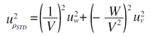 | (10) |
Where
W and
V are weight (g) and volume (cm
3) of STD respectively. There are no correlation between W and V.
The standard uncertainty of weight and volume are combined by type A and B evaluation respectively.
 | (11) |
 | (12) |
The standard uncertainty of the product of skeletal density and thickness of STD denoted by uX-STD is represented by the equation.
 | (13) |
Where the uρSTD and utSTD is the standard uncertainty of the density and thickness of STD. Averaged skeletal density of STD is substituted for ρSTD. The tSTD is adopted by largest value of STD, which were applied for estimating analytical curve.
(III) The standard uncertainty of OD in samples (uOD-SA) is defined by combined type A and type B estimation. Type A estimation was selected as uOD-A from maximum experimental standard deviation of Al-bar of X (uOD-A-X) or Y axis (uOD-A-Y) corresponding to coral skeletal analysis area.
 | (14) |
Type B estimation is expressed as OD resolution of ±0.5 (uOD-B). The propagation is represented by the equation.
 | (15) |
The propagation of logarithmical conversion from OD to Y of uOD-SA was expressed as uY-SA.
 | (16) |
The standard uncertainty of the sample derived from combination of analytical curve of two-degree polynomial formula (uY→X) and uY-SA (uX-SA) is calculated from the following equation.
 | (17) |
Matrixes and vectors express each parameter.
 | (18) |
Where n is number of standards used for estimating analytical curve, Xk is X (=ρSTD·tSTD) value of standard k (= 1, 2, … n), and Yk is measured Y (= ln OD) value of standard k . εk denotes the error of the 2-degree polynomial. Then, â, b̂, ĉ are estimators of a, b, c respectively, and α̂ is estimator of vector α calculated by least square method.
 | (19) |
The uncertainties of â, b̂, ĉ are expressed by ua, ub, uc, which are estimated by the following equations. u2a, u2b, u2c are diagonal components of Eq. (20).
 | (20) |
 | (21) |
In general, the law of propagation is expressed by following equation if there is correlation between xi and xj.
 | (22) |
Estimated correlation coefficient between
xi and
yi(
i<
j) is denoted by
r(
xi,
xj). The estimated covariance of
xi and
xj is denoted by
u(
xi,
xj).
u(
xi,
xj) were expressed the following equation.
 | (23) |
When  and V is expressed as variance -covariance matrix of u(xi,xj) (u(xi,xi) = u2(xi)). The uc(y)of Eq. (22) is expressed by the following equation.
 | (24) |
In Eq. (2), there is correlation among X. To evaluate the uX-SA, Eq. (2) converts to liner equation from non-liner one.
 | (25) |
Then, the uX-SA is expressed by the following equations.
 | (26) |
 | (27) |
 | (28) |
and,
 | (29) |
In this study, XSA and YSA are defined as one time analysis. We referred to web site of Dr. Shirono K. (National Institute of Advanced Industrial Science and Technology, JAPAN; http://staff.aist.go.jp/k.shirono/index_e.html) for the calculation program of (III) section.
(IV) The uX-SA is represented by the propagation in the following equation.
 | (30) |
The uρSA is represented and the following equation.
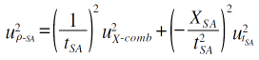 | (31) |
The t and XSA are treated as individual quantity.
4. Results and Discussions
4.1 The coral skeletal density analysis by TATSCAN-X1
Stable isotopic and X-radiography evidence indicated that skeleton of greatest skeletal density was supposed as deposited in winter and did not show any evidence of sub-annual banding by cyclic variation of the oxygen isotope (Fig. 2). If we would compare coral growth and environmental data, we should check the depositional timing of coral skeleton for each slab or at least one slab at each site where environmental variation would be same.
The skeletal density, annual extension rate and calcification rate were measured based on chronology developed by oxygen isotope. Skeletal densities changed from 1.45 to 1.70 g/cm3 and uρSA were ca. 0.02 g/cm3 (Table 1). Annual extension rate changed from 0.149 to 0.468 cm/year and calcification rate did from 0.237 to 0.722 g/cm2/year (Table 1).
Table 1.
Summary of annual coral growth with uncertainty.
| Year |
Skeletal density (g/cm3) |
Uncertainty of skeletal density (g/cm3) |
Extension rate (cm) |
Calcification rate
(g/cm2/year) |
| 2008 |
1.45 |
0.02 |
0.340 |
0.494 |
| 2007 |
1.59 |
0.02 |
0.149 |
0.237 |
| 2006 |
1.54 |
0.02 |
0.468 |
0.722 |
| 2005 |
1.54 |
0.02 |
0.372 |
0.572 |
| 2004 |
1.60 |
0.02 |
0.351 |
0.561 |
| 2003 |
1.66 |
0.02 |
0.330 |
0.548 |
| 2002 |
1.70 |
0.02 |
0.383 |
0.652 |
Table 2 indicate the standard uncertainty and its factor of coral skeletal density collected at 200 m from inshore in 2008 as a typical rate. The 93.7% of uρSA was explained by uX-comb. The uX-SA was mainly originated from uY→X, which was 78.5% of uρSA. Any studies did not consider contribution of uY→X. We will improve uY→X because it depends on the preparation of standard conditions such as thickness.
Table 2.
Summary of contribution of each standard uncertainty for
uρSA.
| Evaluaiton type |
Growth parameter |
Uncertainty (u) |
Rate(%) |
|
Skeletal density (g/cm3; uρ-SA) |
1.75E-02
Squre of sensitivity coefficients * uncertainty |
100.0 |
| (A) |
Sample thickness (cm; ut-SA) |
4.39E-03 |
6.3 |
| (B) |
Deducing of analytical curve +STD(uX-comb) |
1.70E-02 |
93.7 |
| (B-1) |
Deducing of analytical curve (X; uX-SA) |
1.61E-02 |
84.8 |
| (B-2) |
STD uX-STD |
5.23E-03 |
8.9 |
| (B-1-1) |
Deducing of analytical curve (uY→x) |
1.55E-02 |
78.5 |
| (B-1-2) |
Type B (uOD-B) |
2.77E-03 |
2.5 |
| (B-1-3) |
Al-bar(uOD-A) |
3.44E-03 |
3.8 |
| (B-2-1) |
Thickness of STD(utSTD) |
5.60E-04 |
0.1 |
| (B-2-2) |
Density of STD(utSTD) |
5.20E-03 |
8.8 |
On the other hand, utSA would enhance uρSA although the 6.3% of uρSA was explained by utSA. We calculated contribution of utSA in uρSA calculated from eq.(31) (Fig. 3). The relative utSA was changed from ca. 0.23 to 4.0%. Then, uρSA was changed from ca. 0.0175 to 0.05 g/cm3, which were corresponding to the contribution from 6 to 88.5% in uρSA. This indicates that utSA was one of the main factors for uρSA. Depend on study goals, we have to pay attention to the utSA. Our protocol for estimating uρSA basically enables to apply to γ-densitometry and CT analysis. Future research should estimate the uncertainties of coral growth to compare its information and machine conditions.

In this report, we did not show the uncertainty of extension rate and calcification rate. Most studies did not estimate coral extension rate and calcification rate because it was suggested that coral slab was collected perpendicular to the main vertical growth axis of the colony and the there were small uncertainty (e.g. Knutson et al., 1972). If we use the hypothesis, we would calculate the uncertainty of extension rate by digital resolution and that of calcification rate by propagation of uncertainty of skeletal density and extension rate. However, Le Tissier et al. (1994) indicated that errors of density band related to coral growth parameters analyzed by X- radiography may be caused from (1) coral slab not following the growth axis of the colony, and (2) changes in corallite orientation. Although recent studies select and analyzed the maximum coral extension rate by CT to avoid the errors of density band (Carilli et al., 2012; Cantin et al., 2010), they did not clear the uncertainty of extension rate. Further basic studies for estimating uncertainty of coral growth would be needed in the future.
This study reported the new protocol for estimating uρSA by TATSCAN-X1, developed at JAMSTEC, for the first time. Our results indicate that the uρSA is derived from the combined effects of 78.5% from uY→X, and 6.3% from utSA. The utSA depends on cutting technique of coral skeleton. The coral core center, constructed in Hokkaido University, Japan, had the machine for cutting the flattened coral slab with 100μm interval. If we use the machine and TATSCAN-X1, we would get the minimum uncertainty of skeletal density.
Acknowledgments
We thank to Mr. Jumpei Isasa, Suguru Kawamura and Masataka Ikeda for field assistance. We also thank to Mr. Koichi Iijima for research advice. The authors acknowledge Hidehiko Nomura, Kosuke Nakamura at Thin Section Technician's Lab, Hokkaido University for technical advising of sample preparation. The authors are grateful to Dr. Kazumasa Oguri and to anonymous reviewers for their corrections and comments, which help improving that manuscript.
References
- Bessat, F. and D, Buigues (2001), Two centuries of variation in coral growth in a massive Porites colony from Moorea (French Polynesia): a response of ocean-atmosphere variability from south central Pacific, Paleogeogr. Paleoclimatol. Paleoecol., 175, 381-39.
- Bosscher, H (1993), Computerized tomography and skeletal density of coral skeleton, Coral Reefs, 12, 97-103.
- Cantin, N. E., A. L. Cohen, K. B. Karnauskas, A. M. Tarrant, and D. C. McCorkle (2010), Ocean Warming Slows Coral Growth in the Central Red Sea, Science, 329, 322-325.
- Carilli, J. S. D.Donner , and A. C. Hartmann (2012), Historical temperature variability affects coral response to heat stress, PLoS ONE, 7, e34418.
- Carlton, R. R. and A. M. Adler (1996). Principles of Radiographic Imaging. 2nd ed., Delmar Pub.
- Carricart-Ganivet, J. P., and D. J. Barnes (2007), Densitometry from digitized images of X-radiographs: Methodology for measurement of coral skeletal density, J Exp Mar Biol Ecol, 344, 67-72.
- Carricart-Ganivet, J. P., N. Cabanillas-Terán, I. Cruz-Ortega, and P. Blanchon (2012), Sensitivity of calcification to thermal stress varies among genera of massive reef-building corals, PLoS ONE, 7, e32859.
- Castillo, K. D., J. B. Ries, and J. M. Weiss (2011), Declining coral skeletal extension for forefeef colonies of Siderastrea siderea on the Mesoamerican Barrier Reef system, southern Belize, PLoS ONE, 6, e14615.
- Chalker, B. E. and D. J. Barnes (1990), Gamma densitometry for the measurement of coral skeletal density, Coral Reefs, 9, 11-23.
- Cooper, T. F., G. De'ath, K. E. Fabricius, and J. M. Lough (2008), Declining coral calcification in massive Porites in two nearshore regions of the northern Great Barrier Reef, Global Change Biol.,14, 529-538.
- Cooper, T. F., R. A. O'Leary, and J. M. Lough (2012), Growth of Western Australian corals in the anthropocene, Science, 335, 593-596.
- De'ath, G., J. M. Lough, and K. E. Fabricius (2009) Declining Coral Calcification on the Great Barrier Reef, Science, 323, 116-119.
- ISO/IEC Guide 98-3, (2008), Uncertainty of measurement-Part3 : Guide to the expression of uncertainty in measurement (GUM : 1995), Evaluation of measurement data-Guide to the expression of uncertainty in measurement, JCGM 100.
- Hart, D. E. and P. S. Kench (2006), Carbonate production of an emergent reef platform, Warraber Island, Torres Strait, Australia, Coral Reefs., 26, 53-68.
- Helmle, K. P., R. E. Dodge, P. K. Swart, D. K.Gledhill, C. and M. Eakin, (2011), Growth rates of Florida corals from 1937 to 1996 and their response to climate change, Nat. Commun., 2, 215.
- Klein, R., J. Patzold, G. Wefer, and Y. Loya (1993), Depth-related timing of density band formation in Porites spp. corals from the Red-Sea inferred from X-ray chronology and stable-isotope composition, Mar Ecol Prog Ser., 97, 99-104.
- Knutson, R. A., R. W. Buddemeier, and S. V. Smith (1972), Coral chronometers: seasonal growth bands in reef corals, Science, 177, 270-272.
- Le Tissier, M. D., B. Clayton, B. E. Brown, and P. S. Davies (1994), Skeletal correlates of density banding and an evaluation of radiography as used in sclerochronology, Mar. Ecol. Prog. Ser., 110, 29-44.
- Langdon, C. and M. J. Atkinson (2005), Effect of elevated pCO2 on photosynthesis and calcification of corals and interactions with seasonal change in temperature/irradiance and nutrient enrichment, J. Gephys. Res-Oceans., 10, doi:10.1029/2004JC002576.
- Lough, J. M. and D. J. Barnes (1990), Intra-annual timing of density band formation of Porites coral from the central Great Barrier Reef, J. Exp. Mar. Biol. Ecol., 135, 35-57.
- Lough, J. M. and T. F. Cooper (2011), New insights from coral growth band studies in an era of rapid environmental change, Earth-Sci Rev., 108, 170-184.
- Miller, J. C. and J. N. Miller (1988), Statistics for Analytical Chemistry, 2nd ed., Ellis Horwood.
- Rosenfeld, M., R. Yam, A. Shemesh, and Y. Loya (2003), Implication of water depth on stable isotope composition and skeletal density banding patterns in a Porites lutea colony: results from a long-term translocation experiment, Coral Reefs, 22, 337-345.
