The OJP array: seismological and electromagnetic observation on seafloor and islands in the Ontong Java Plateau

Abstract

We conducted geophysical observations on the Ontong Java Plateau (OJP) and its vicinity from late 2014 to early 2017 to determine the underlying crust and upper mantle structure beneath the OJP. Most of the OJP was emplaced in the present South Pacific region at 122 Ma by massive volcanism, but the origin of this volcanism are still debated. Previous studies have suggested that seismic velocity beneath the OJP is anomalously slow, thus this could represent thermal or chemical remnants of the volcanism. However, the seismic resolution of the slow anomalies is poor due to lack of seafloor observations. The observation network named “the OJP array” is composed of seafloor and island stations. The seafloor stations have broadband ocean bottom seismographs and ocean bottom electromagnetometers. The island stations have broadband seismographs. The OJP array is designed to obtain seismic and electrical conductivity structures of the mantle beneath the OJP with better resolution than that of previous studies. Joint analysis and interpretation of seismological and electromagnetic data should provide tight constraints to thermal and chemical structures and clarify the origin of OJP emplacement.

1. Introduction

The Ontong Java Plateau (OJP) is the most voluminous Large Igneous Provinces in the oceanic region of the Earth (Fig. 1). The area of the OJP is $1.6 \times 10^{6}$ km², and the elevation is approximately 2000 m above the surrounding seafloor. The OJP was emplaced at 122 and 90 Ma by massive volcanism, with the 122 Ma event seeming to be significantly larger than 90 Ma event (e.g., Coffin and Eldholm, 1994; Neal et al., 1997). The volcanic eruption had a major effect on the Earth's environment, including global climate change, oceanic anoxic events, and mass extinction of marine life (e.g., Larson, 1991; Tejada et al., 2009). However, the cause of the volcanism remains controversial. Some studies suggested that a rapid ascent of hot mantle materials from the bottom of the mantle caused the eruption (e.g., Coffin and Eldholm, 1994). Others hypothesized that the mantle upwelling responsible for the eruption could be of shallow origin (Korenaga, 2005). One reason for the poor understanding of the origin of the OJP is the lack of information about the crust and mantle structure beneath the OJP.

Fig.1.

Geographical location of the OJP and hypocenters with magnitudes larger than 5.5 (red crosses) during this observation period. (a) observation region is indicated by a rectangle. (b) Station distribution of the OJP array. Orange triagles are equipped with both of BBOBS and OBEM. The white triangles have only BBOBSs. BBOBS stations with DPGs are indicated by double triangles. The BBOBS equipped with long anchors are shown in black crosses. The stations CHUK and KOSR (red triangles) are located on Chuuk and Kosrae islands, respectively. The background color indicates the topography in meters. The OJP is roughly defined by a region whose water depth is shallower than 4000 m (white contour line) and its approximate boundary with the Solomon Islands to the southwest.

Previous active seismic experiments have revealed that the crust beneath the OJP is 35-45-km thick (e.g., Furumoto et al., 1976; Gladczenko et al., 1997; Miura et al., 2015). However, these survey lines covered only a portion of the broad OJP region. Previous studies of mantle tomography using seismological data from islands in the region surrounding the OJP indicated the presence of a broad, low-velocity zone between 100-300 km beneath the entire OJP region (Richardson et al., 2000; Covellone et al., 2015). Thermal anomalies alone were difficult to explain the low-velocity zone because a remnant of the OJP in the upper mantle, if any, should have cooled since its emplacement at 122 and 90 Ma (Tharimena et al., 2016). Gomer and Okal (2003) determined weak seismic attenuation beneath the OJP from ScS wave analysis, suggesting that the low-velocity anomalies were not due to thermal anomalies because the high-temperature anomalies were accompanied by high attenuation. Compositional anomalies that explain the low-velocity anomalies have not been identified due to poor information of the upper mantle structure beneath the OJP because of lack of long-term seafloor observations. Joint analysis and interpretation of seismological and electromagnetic data could resolve the thermal and compositional anomalies. No seismological or electromagnetic observations have been performed on the OJP seafloor, except for the active-seismic experiments, before the current study.

We conducted the first seismological and electromagnetic observations on the seafloor and islands of the OJP between 2014 and 2017 to overcome the previously described difficulties (Fig. 1). We call the observation network collectively as the OJP array. The primary mission of the project was to determine the crust and upper mantle structures beneath the OJP with unprecedented spatial resolution. The advantage of the OJP array was the capability to determine both seismic and electrical conductivity structures, which were essential for understanding the OJP origin. We provided details of the observation instruments, deployment methods, and data quality of the OJP array in the current report.

2. Instruments

2.1 Broadband ocean bottom seismograph (BBOBS) and land-based seismograph

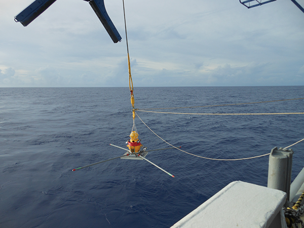
The BBOBS system used in the current study (Fig. 2) was developed as a portable, broadband, ocean bottom instrument (Kanazawa et al., 2001; Shiobara et al., 2009) under the Ocean Hemisphere network Project, 1996-2001 (Fukao et al., 2001). The BBOBS system was suitable for studying the crust and upper mantle structures beneath the OJP, because the system can sense and record ground motions of long-period seismic waves traveling deep in the mantle (e.g., Suetsugu and Shiobara, 2014), as explained in section 5. We have conducted more than 150 long-term ocean bottom seismograph (OBS) experiments since 1999 (e.g., Suetsugu et al., 2005; Shiobara et al., 2009; Suetsugu et al., 2012; Matsuno et al., 2017).

Fig.2.

Outer view of the BBOBS unit (not equipped with long anchor or DPG).

BBOBS units were deployed by free fall and recovered with a self-pop-up system that allowed them to rise from the seafloor upon receipt of an acoustic command. The three-component CMG-3T broadband sensor (Guralp Systems Ltd.) used in the BBOBS housing sensed ground motion at periods from 0.02 to 360 s. The data logger (LS-9100; Hakusan Ltd.) has a sampling rate of 100 Hz at a 24-bit resolution. All of the seismic instrument components including the sensor, data logger, transponder (SI-2; Kaiyodenshi Ltd.), and batteries (Li-cells) were packed into a 65-cm-diameter titanium alloy pressure housing that allowed for a maximum operating depth of 6000 m. The BBOBSs at the OJ02, OJ06, OJ08, OJ11, and OJ14 sites were equipped with differential pressure gauges (DPGs) (Araki and Sugioka, 2009) to improve signal-to-noise ratios (S/N) of earthquake ground motions. The BBOBSs at the OJ02, OJ06, OJ08, OJ11, OJ13, and OJ14 sites were equipped with longer anchors than normal to improve their coupling with the ground and designed to reduce ground noise at frequencies of approximately 0.01 Hz effectively (Ito et al., 2009). The system ran for 1.5 years to ensure the capture of numbers of earthquakes for further data analysis.

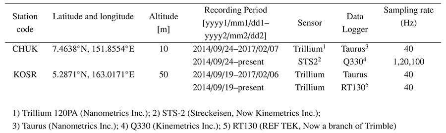
The broadband seismographs on the islands comprised broadband STS-2 (Streckeisen AG) and Trillium 120PA (Nanometrics Inc.) seismic sensors and Taurus (Nanometrics Inc.), Q330 (Quanterra Inc.), and RT130 (REF TEK Inc.) data loggers, which recorded ground motion continuously at period from 0.05 s to 120 s with a sampling rate of 40 Hz and a 24-bit resolution. Figure 3 shows the seismic vault and sensor at the CHUK station.

Fig.3.

Broadband seismological station CHUK in Chuuk island.

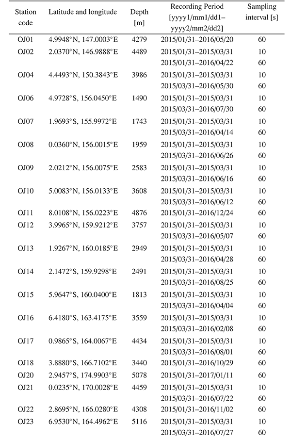
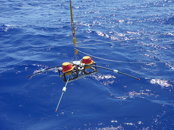
2.2 Ocean-bottom electromagnetometer (OBEM)

The OBEM systems measured time variations of three components of the magnetic field, horizontal electrical field, instrumental tilts, and temperature. The magnetic and electrical fields were analyzed to determine electrical conductivity structure. Most of the OBEMs recorded data with a sampling interval of 10 s for the first two months, and then the interval was switched to 60 s for the rest of the observation period. Data at 10 and 60 s intervals were useful to constrain crust and upper mantle structures, respectively (Baba et al., 2017). The resolution was 0.01 nT for the fluxgate magnetometer, 0.305 $\mu $V using a 16-bit A/D converter or 0.01 $\mu $V using a 24-bit A/D converter for the voltmeter, $2.6 \times 10^{-4}$° for the tiltmeter; and 0.01℃ for the thermometer. We used a two-glass sphere-type OBEM (Type A; Fig. 4a) and a one-glass sphere-type OBEM (Type B; Fig. 4b). The Type A system had two pressure-resistant, 17-inch-thick-glass spheres. One sphere contained the magnetic sensors and recorder, and the other contained an acoustic transponder and a lithium battery pack. The Type B system comprised one pressure-resistant, 17-inch-thick-glass sphere, a sensor unit in a titanium pressure housing, an acoustic transponder unit, and an electrode arm unit with an arm-holding mechanism that folded the electrode arms when the OBEM was surfacing (Kasaya et al., 2009; Kasaya and Goto, 2009). The glass sphere contained a data logger and a lithium battery pack. Each OBEM had four pipes for attaching five Filloux-type silver-silver chloride electrodes (Clover Tech Inc.) (Filloux, 1987).

Fig.4.

Outer view of the OBEM units. (a) Two-glass sphere-type OBEM.

Fig.4.

Outer view of the OBEM units. (b) one-glass sphere-type OBEM.

3. Deployment and recovery of the instruments

We installed 23 BBOBSs and 20 OBEMs between November 2014 and January 2015 on the seafloor at depths of 1500-5100 m beneath sea level (mbsl) from the research vessel MIRAI of the Japan Agency for Marine-Earth Science and Technology (JAMSTEC) (Fig. 1). Before installation, we performed a bathymetry survey with a multi narrow-beam echo sounder on an area of 15-20 nautical square miles (nm) around the planned installation locations. Detailed bathymetry data was essential to determine electrical conductivity structures under the seafloor accurately (e.g., Baba et al., 2013). All the instruments were recovered between January and February 2017 by the JAMSTEC research vessel HAKUHO-MARU. All instruments were operational for approximately 1.5 years except five BBOBSs (OJ01, OJ10, OJ17, OJ21, and OJ23) that stopped working because of hardware malfunctions.

We also installed two temporary broadband seismological stations in September 2014 on the Chuuk and Kosrae Islands of the Federated States of Micronesia, which are located directly north of the OJP (CHUK and KOSR in Fig. 1). We deployed two independent seismographs on each island to secure continuous observations. Observations by the systems employing Taurus recorders were completed in January and February 2017. The other systems are still in operation. Detailed information of the stations in the OJP array is provided in Tables 1-3.

Table 1. BBOBS locations and recording periods.

Station code	Latitude and longitude	Depth [m]	Recording Period [yyyy1/mm1/dd1-yyyy2/mm2/dd2]	Additional equipment
OJ01	4.9957°N, 147.0005°E	4275	-	-
OJ02	2.0380°N, 146.9911°E	4486	2015/01/08-2016/09/29	Long anchor, DPG
OJ03	0.0588°N, 147.0352°E	4486	2015/01/09-2016/09/30	-
OJ04	4.4500°N, 150.3830°E	3987	2014/12/17-2016/09/05	-
OJ05	0.6155°S, 153.0019°E	4337	2014/12/10-2016/08/30	-
OJ06	4.9730°S, 156.0448°E	1491	2014/12/26-2016/09/14	Long anchor, DPG
OJ07	1.9712°S, 155.9971°E	1743	2016/08/20-2016/09/16	-
OJ08	0.0362°S, 156.0005°E	1959	2014/12/30-2016/09/20	Long anchor, DPG
OJ09	2.0216°N, 156.0074°E	2583	2015/01/01-2016/09/22	-
OJ10	5.0093°N, 156.0128°E	3608	-	-
OJ11	8.0129°N, 156.0245°E	4875	2015/01/04-2016/09/25	Long anchor, DPG
OJ12	4.0016°N, 159.9176°E	3756	2014/12/22-2016/09/11	-
OJ13	1.9263°N, 160.0164°E	2948	2014/12/23-2016/09/13	Long anchor
OJ14	2.1477°S, 159.9271°E	2491	2014/12/24-2016/09/14	Long anchor, DPG
OJ15	5.9649°S, 160.0408°E	1813	2014/12/07-2016/08/26	-
OJ16	6.4173°S, 163.4168°E	3558	2014/12/05-2016/08/25	-
OJ17	0.9852°S, 164.0086°E	4435	-	-
OJ18	3.8879°S, 166.7082°E	3441	2015/03/01-2016/08/18	-
OJ19	8.0121°S, 170.0532°E	4860	2014/11/24-2016/08/15	-
OJ20	2.9458°S, 174.9907°E	5077	2014/11/19-2016/08/10	-
OJ21	0.0259°N, 170.0046°E	4458	-	-
OJ22	2.8711°N, 166.0263°E	4309	2014/11/17-2016/08/07	-
OJ23	6.9544°N, 164.4966°E	5117	-	-

Table 2.

Broadband seismographs located on islands.

Table 3.

OBEM locations and recording periods.

4. Data

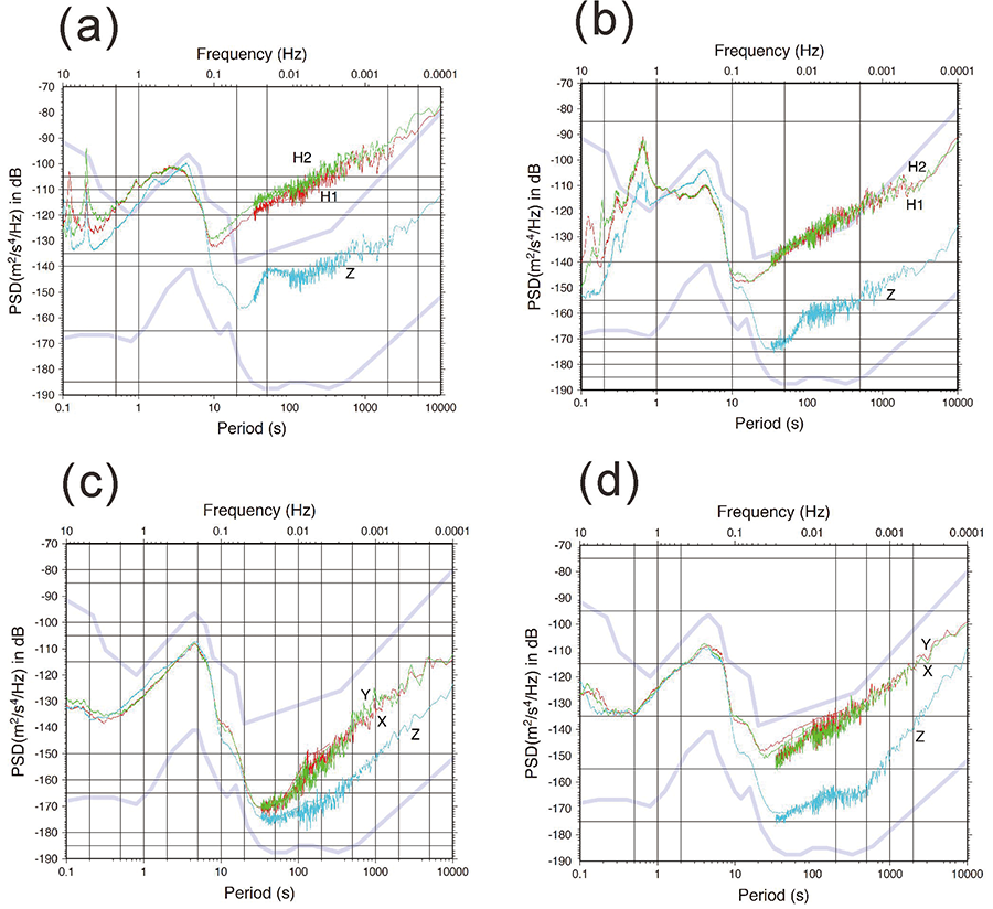
4.1 Seismic noise level

Figures 5a and 5b show the noise levels at the BBOBS sites OJ06 and OJ11 as examples of high and low-noise sites, respectively. Vertical-component noise at OJ06 was lower than the New High Noise Model (Peterson, 1993) by approximately 15 dB and that at OJ11 was approximately midway between the New High and Low Noise Models. The Models were developed with ground acceleration data from globally distributed stations and were regarded as the range of noise levels on the land area of the globe. Horizontal-component noises are greater than the New High Noise Model at OJ06 and similar to the Model at OJ11. The higher noise level of the horizontal components was probably caused by ocean-bottom currents directly pushing and tilting the BBOBS on the seafloor (e.g., Webb, 1988). We found no obvious noise level dependency on station location or between instruments with long and short anchors. Figures 5c and 5d show noise levels at the island stations, CHUK and KOSR, indicating much lower noise levels than those at the BBOBS sites. In particular, noise levels at CHUK were exceptionally low for an island station. The CHUK stations were located in a tunnel drilled into hard volcanic rock in a relatively quiet lagoon (Fig. 3), which might have contributed to the low-noise levels at CHUK.

Fig.5.

Examples of noise models for the BBOBS stations and island stations. (a) OJ06; (b) OJ11; (c) CHUK; and (d) KOSR. Averaged noise spectra during the entire deployment period except from time windows of known earthquakes are shown. The vertical component is shown by blue curves and the horizontal-component (H1 and H2 in (a) and (b); X, Y in (c) and (d)) are shown by red and green curves. The New High Noise Model and the New Low Noise Model (Peterson, 1993) are also shown as pale-colored, thick curves.

4.2 Examples of seismograms

During this 630-day observation, more than 800 earthquakes larger than magnitude (Mw and Ms) 5.5 occurred worldwide. Examples of raw seismograms for a shallow earthquake (11-km deep, Ms 6.8) in the Solomon Islands are presented in Fig. 6. Clear seismic phases, including P, S, and surface waves, were recorded. The data quality was sufficient for the planned data analyses as described in section 5.

Fig.6.

Seismograms recorded by the OJP array for shallow earthquakes (11-km deep) in the Solomon Islands during May 2015 (M6.8). (a) Epicenter and great circle paths between the epicenter and the stations of the OJP array. A vertical component (b) and two horizontal components (c, d) are shown. Theoretical traveltime curves predicted by the iasp91 model (Kennett and Engdahl, 1991) are also shown by red lines. No filter is applied.

4.3 Example of OBEM records

The OBEMs continuously recorded magnetic and electric fields. Representative records at the OJ17 site are shown in Fig. 7. High-frequency oscillations in the magnetic data (top four panels) represented daily magnetic variations. Long-period signals with abrupt onsets and long tails were signals produced by magnetic storms, which were used along with electrical signals to determine electrical conductivity structures.

Fig.7.

Raw time-series data collected from the OBEM site OJ17. From top to bottom, the panel shows the total magnetic field intensity B$_{total}$ calculated from the three components of the magnetic field plotted below (upper two components B1 and B2, are nearly horizontal and the third component, B3, is nearly vertical), the two components of the instrumental tilt ($\theta $pitch is the angle of elevation in 1-3 axes plane and $\theta $roll is the angle of dip in 2-3 axes plane), four voltage differences between four electrodes and a reference electrode, and the temperature of the data logger circuit Tc.

5. Planned analysis of data

We plan to apply seismic tomography to the data from the OJP array and permanent seismic stations located in the Pacific Ocean to determine three-dimensional seismic velocity structures of the upper mantle beneath the OJP using body wave traveltime tomography (e.g., Obayashi et al., 2016) and surface wave tomography (e.g., Isse et al., 2016) with unprecedented spatial resolution. The lateral and vertical extents of the previously found low-velocity zone and the geophysical nature are key questions that will be solved by tomography. The ability to determine both seismic and electrical conductivity structures beneath the OJP is an advantage of the array. The OBEM data will be analyzed using a three-dimensional magnetotelluric method (Tada et al., 2014; 2016) to obtain the electrical conductivity structure of the upper mantle. The conductivity is more sensitive to an abundance of volatiles (e.g., H₂O and CO₂) and a degree of partial melting than seismic velocity, but seismic velocity is sensitive to temperature. Simultaneous use of BBOBS and OBEM data could provide information on temperature, the degree of partial melting, and the abundance of volatiles to elucidate the cause of the low-velocity zone. We will map the depths of the Moho, the lithosphere-asthenosphere boundary, and the 410- and 660-km-deep discontinuities beneath the OJP using a receiver function method (e.g., Owens and Crosson, 1988; Suetsugu et al., 2010). Two-dimensional variation of the Moho depth will be used to estimate the volume of the erupted magma. An ascending mantle flow that generated the OJP may have interacted with the pre-existing lithosphere during the eruption (Ishikawa et al., 2004), which may remain in the lithosphere-asthenosphere boundary at present. The 410- and 660-km-deep discontinuities will be useful to determine whether the low-velocity anomaly is confined to the upper mantle or rooted deeper in the mantle transition zone. This complete view of the crust and upper mantle structures beneath the OJP will provide important information about the origin of the OJP.

Acknowledgments

We thank the captains, officers, and crew of JAMSTEC's R/V MIRAI and R/V HAKUHO-MARU for successful operation during the deployment and recovery cruises of the BBOBS and OBEM. The present study was partially funded by JSPS KAKENHI, Grant Number 15H03720.

References

•     Araki,  E . and  H.  Sugioka (2009), Calibration of deep sea differential pressure gauge, JAMSTEC Rep. Res. Dev., Special Issue, 141-148.
•     Baba,  K. ,  N.  Tada ,  H.  Utada , and  W.  Siripunvaraporn (2013), Practical incorporation of local and regional topography in three-dimensional inversion of deep ocean magnetotelluric data, Geophys. J. Int., 194, 348-361, doi:10.1093/gji/ggt115.
•     Baba,  K. ,  N.  Tada ,  T.  Matsuno ,  P.  Liang ,  R.  Li ,  L.  Zhang ,  H.  Shimizu ,  N.  Abe ,  N.  Hirano ,  M.  Ichiki , and  H.  Utada (2017), Electrical conductivity of old oceanic mantle in the northwestern Pacific I: 1-D profiles suggesting differences in thermal structure not predictable from a plate cooling model, Earth, Planets and Space, 69, doi:10.1186/s40623-017-0697-0.
•     Coffin,  M. and  O.  Eldholm (1994), Large Igneous provinces: crustal structure, dimensions, and external consequences, Rev. Geophys., 32, 1-36.
•     Covellone,  B. M. ,  B.  Savage , and  Y.  Shen (2015), Seismic wave speed structure of the Ontong Java Plateau, Earth Planet. Sci. Lett., 420, 140-150.
•     Filloux,  J.H. (1987), Instrumentation and experimental methods for oceanic studies, In: J. Jacobs (Editor): New Volumes on cil of Canada, Collaborative Special Grant A6892; Geomagnetism and Geoelectricity, Vol. I. Academic Press, New York, 143-245.
•     Fukao,  Y. ,  Y.  Morita ,  M.  Shinohara ,  T.  Kanazawa ,  H.  Utada ,  H.  Toh ,  T.  Kato ,  T.  Sato ,  H.  Shiobara ,  N.  Seama ,  H.  Fujimoto , and  N.  Takeuchi (2001), The Ocean Hemisphere Network Project (OHP), In: B. Romanowicz, K. Suyehiro, and H. Kawakatsu (Eds.), OHP/ION joint symposium workshop report, 13-29.
•     Furumoto,  A.S. ,  J.P.  Webb ,  M.E.  Odegard , and  D.M.  Hussong (1976), Seismic studies on the Ontong Java Plateau, 1970, Tectonophysics, 34, 71-90.
•     Gladczenko,  T. P. ,  M. F.  Coffin , and  O.  Eldholm (1997), Crustal structure of the Ontong Java Plateau: Modeling of new gravity and existing seismic data, J. Geophys. Res., 102, 22711-22729.
•     Gomer,  B. and  E.  Okal (2003), Multiple-ScS probing of the Ontong-Java Plateau, Phys. Earth Planet. Inter., 138, 317-331.
•     Ishikawa,  A. ,  S.  Maruyama , and  T.  Komiya (2004), Layered lithospheric mantle beneath the Ontong Java Plateau: implications from xenoliths in Alnoite, Malaita, Solomon islands, J. Petrol., 45, 2011-2044.
•     Isse,  T. ,  H.  Sugioka ,  A.  Ito ,  H.  Shiobara ,  D.  Reymond , and  D.  Suetsugu (2016), Upper mantle structure beneath the Society hotspot and surrounding region using broadband data from ocean floor and islands, Earth, Planets and Space, 68, doi:10.1186/s40623-016-0408-2.
•     Ito,  A. ,  H.  Sugioka , and  E.  Araki (2009), An installation experiment with broadband ocean bottom seismometers for reducing low frequency seismic noises, JAMSTEC Rep. Res. Dev., Special Issue, 131-140.
•     Kanazawa,  T. ,  M.  Mochizuki , and  H.  Shiobara (2001), Broadband seismometer for a long-term observation on the sea floor, Proceedings of the OHP/ION Joint Symposium on Long-term observations in the oceans: current status and perspectives for the future, OP-05.
•     Kasaya,  T. ,  T.  Goto ,  K.  Baba ,  M.  Kinoshita ,  Y.  Hamano , and  Y.  Fukao (2009), Recent progress of the Electro-Magnetic survey to investigate Earth's interior, JAMSTEC Rep. Res. Dev., Special Issue, 103-110.
•     Kasaya,  T. and  T.  Goto (2009), A small ocean bottom electromagnetometer and ocean bottom electrometer system with an arm-folding mechanism (Technical Report). Exploration Geophys., 40(1), 41-48, doi:10.1071/EG08118.
•     Kennett,  B.L.N. and  E. R.  Engdahl (1991), Traveltimes for global earthquake location and phase identification, Geophys. J. Int., 105, 429-465, doi:10.1111/j.1365-246X.1991.tb06724.x.
•     Korenaga,  J. (2005), Why did not the Ontong Java Plateau form subaerially?, Earth Planet. Sci. Lett., 234, 385-399.
•     Larson,  R. (1991), Latest pulse of earth: evidence for a mid-cretaceous superplume, Geology, 19, 547-550.
•     Matsuno,  T. ,  D.  Suetsugu ,  K.  Baba ,  N.  Tada ,  H.  Shimizu ,  H.  Shiobara ,  T.  Isse ,  H.  Sugioka ,  A.  Ito ,  M.  Obayashi ,  H.  Utada (2017), Mantle transition zone beneath a normal seafloor in the northwestern Pacific: Electrical conductivity, seismic thickness, and water content, Earth and Planet. Sci. Lett., 462, 189-198.
•     Miura,  S. ,  G.  Fujie ,  T.  Shirai ,  N.  Noguchi ,  S.  Kodaira ,  M. F.  Coffin ,  S. A.  Kawagle , and  R.  Verave (2015), Crustal thickness of the Ontong Java Plateau and deep reflections near the base of its crust, 2015 AGU Fall Meeting Abstract, V21A- 3026.
•     Neal,  C. ,  J.  Mahoney ,  L.  Kroenke ,  R.  Duncan , and  M.  Petterson (1997), The Ontong Java Plateau, In: J. J. Mahoney and M. F. Coffin (Eds.), Large Igneous Provinces: Continental, Oceanic, and Planetary, Flood Volcanism, (Geophysical Monograph Series 100), 183-216.
•     Obayashi,  M. ,  J.  Yoshimitsu ,  H.  Sugioka ,  A.  Ito ,  T.  Isse ,  H.  Shiobara ,  D.  Reymond , and  D.  Suetsugu (2016), Mantle plumes beneath the South Pacific superswell revealed by finite frequency P tomography using regional seafloor and island data, Geophys. Res. Lett., 43, doi: 10.1002/2016GL070793.
•     Owens,  T. J. and  R. S.  Crosson (1988), Shallow structure effects on broadband teleseismic P waveforms, Bull. Seismol. Soc. Am., 78, 96-108.
•     Peterson,  J. (1993), Observations and modeling of seismic background noise, U.S. Geol. Surv. Open-File Rept. 93-322.
•     Richardson,  W. ,  E.  Okal , and  S.  Van der Lee (2000), Rayleigh-wave tomography of the Ontong-Java Plateau, Phys. Earth Planet. Inter., 118, 29-51.
•     Shiobara,  H. ,  K.  Baba ,  H.  Utada , and  Y.  Fukao (2009), Ocean bottom array probes stagnant slab beneath the Philippine Sea, EOS Trans. AGU, 90, 70-71.
•     Suetsugu,  D. ,  H.  Shiobara ,  H.  Sugioka ,  G.  Barruol ,  F.  Schindele ,  D.  Reymond ,  A.  Bonneville ,  E.  Debayle ,  T.  Isse ,  T.  Kanazawa , and  Y.  Fukao (2005), Probing South Pacific mantle plumes with ocean bottom seismographs, Eos Trans. AGU, 86, 429-435.
•     Suetsugu,  D. ,  T.  Inoue ,  M.  Obayashi ,  A.  Yamada ,  H.  Shiobara ,  H.  Sugioka ,  A.  Ito ,  T.  Kanazawa ,  H.  Kawakatsu ,  A.  Shito , and  Y.  Fukao (2010), Depths of the 410-km and 660-km discontinuities in and around the stagnant slab beneath the Philippine Sea: Is water stored in the stagnant slab?, Phys. Earth Planet. Inter., 183, 270-279.
•     Suetsugu  D. ,  H.  Shiobara ,  H.  Sugioka ,  A.  Ito ,  T.  Isse ,  T.  Kasaya ,  N.  Tada ,  K.  Baba ,  N.  Abe ,  Y.  Hamano ,  P.  Tarits ,  J. P.  Barriot , and  D.  Reymond (2012), TIARES project―tomographic investigation by seafloor array experiment for the Society hotspot, Earth Planets Space, 64, i-iv.
•     Suetsugu,  D. and  H.  Shiobara (2014), Broadband Ocean-Bottom Seismology, Annu. Rev. Earth Planet. Sci., 42, 27-43.
•     Tada,  N. ,  K.  Baba , and  H.  Utada (2014), Three-dimensional inversion of seafloor magnetotelluric data collected in the Philippine Sea and the western margin of the northwest Pacific Ocean, Geochem. Geophys. Geosys., 15, 2895-2917, doi:10.1002/2014GC005421.
•     Tada,  N. ,  P.  Tarits ,  K.  Baba ,  H.  Utada ,  T.  Kasaya , and  D.  Suetsugu (2016), Electromagnetic evidence for volatile-rich upwelling beneath the society hotspot, French Polynesia, Geophys. Res. Lett., 43, 12021-12026, doi:10.1002/2016GL071331.
•     Tejada,  M.L.G. ,  K.  Suzuki ,  J.  Kuroda ,  R.  Coccioni ,  J.J.  Mahoney ,  N.  Ohkouchi ,  T.  Sakamoto , and  Y.  Tatsumi (2009), Ontong Java Plateau eruption as a trigger for the early Aptian oceanic anoxic event, Geology, 37, 855-858, doi:10.1130/G25763A.1
•     Tharimena,  S. ,  C.A.  Rychert , and  N.  Harmon (2016), Seismic imaging of a midlithospheric discontinuity beneath Ontong Java Plateau, Earth Planet. Sci. Lett., 450, 62-70.
•     Webb,  S.C. (1988), Long-period acoustic and seismic measurements and ocean floor currents, IEEE J. Ocean. Eng., 13, 263-270.