Abstract
An absolute quantitative analysis method has been recently developed as a third
generation polymerase chain reaction method “PCR” for fractionated DNA. The method is
designed to determine the number of DNA molecules in target DNA samples by counting the
number of PCR products obtained from fractionated DNA. We applied EXCEL Macro to perform
the conversion of two dimensional orthogonal coordinate (x,
y) fluorescent signal plot data obtained by digital PCR device
to two dimensional polar coordinate (r, θ)
fluorescent signal plot data, followed by analyzing the angle
(θ) histogram of plot data without overlapping of plot
data occurring by two dimensional orthogonal coordinate (x,
y) histogram. The analysis made it possible to identify gene
mutation and count the number of DNA molecules with mutation faster and easier.
1 INTRODUCTION
It has been demonstrated that data from digital PCR analysis [1,2,3,4], in which wild type and mutant type are
labeled with a probe/Hexachloro Fluorescein (HEX) and a probe/Fluorescein Amidite (FAM),
respectively, generate almost 15,000–20,000 fluorescent signals, the results of which are
recorded in the two dimensional orthogonal coordinate (x,
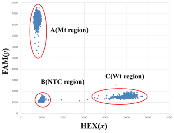
y) to determine the extent of target gene amplification [5]. It is possible to detect the presence of gene mutation
and the rate of mutation with high sensitivity in an extremely small amount of target sample
by plotting the intensity of mutant type (Mt) with HEX fluorescent signal in the
x-axis and wild type (Wt) with FAM fluorescent signal in
the y-axis in two dimensional orthogonal coordinate
(x, y) (Figure 1). It is, however, difficult to show the distribution status
in two dimensional orthogonal coordinate (x,
y) histogram without overlapping of the plots between no DNA
template control (NTC) region and Mt region or NTC region and Wt region, resulting in the
need for two separate histograms created from x (HEX) axis
direction and y (FAM) axis direction. In this study, it is
possible to observe all fluorescent signal plots in angle (θ)
histogram without the overlapping, where the histogram was created based on the value of
angle (θ) of the converted two dimensional polar coordinate
(r, θ) [6], which was prepared by converting from the data in the two dimensional
orthogonal coordinate (x, y) by EXCEL. The
origin of the converted two dimensional polar coordinate (r,
θ) was moved to the gravity point of the triangle consisting of
each center of Mt region, Wt region and NTC region. Therefore, it is possible to determine
gene mutation easily and accurately as well as determine mutation rate by applying the polar
coordinate approach.
2 METHOD AND RESULTS
2.1 Digital PCR data in two dimensional orthogonal coordinate
(x, y)
It has been generally demonstrated that the extent of the target gene amplification could
be monitored by plotting the intensity of fluorescence signals of Wt/HEX in the
x axis and those in Mt/FAM in the
y axis in two dimensional orthogonal coordinate
(x, y). The extent of occurrence
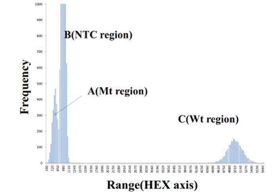
frequency was only determined by histogram. It is, however, difficult to count the
accurate number of Mt/FAM fluorescent signals in x axis
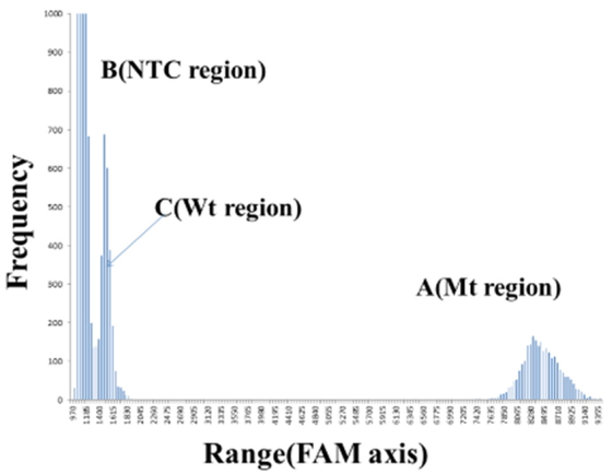
histogram, because of overlapping signals of NTC with those of Mt/FAM (Figure 2). Similarly, it was also difficult to count
the accurate number of Wt/HEX fluorescent signals in y axis
histogram, because of overlapping signals of NTC with those of Wt/HEX (Figure 3). Therefore, the distribution condition of
Mt/FAM and Wt/HEX fluorescent signals by one histogram is difficult to observe in two
dimensional orthogonal coordinate (x, y)
without any overlapping signals.
2.2 Conversion from two dimensional orthogonal coordinate
(x, y) to two dimensional
polar coordinate (r,θ)
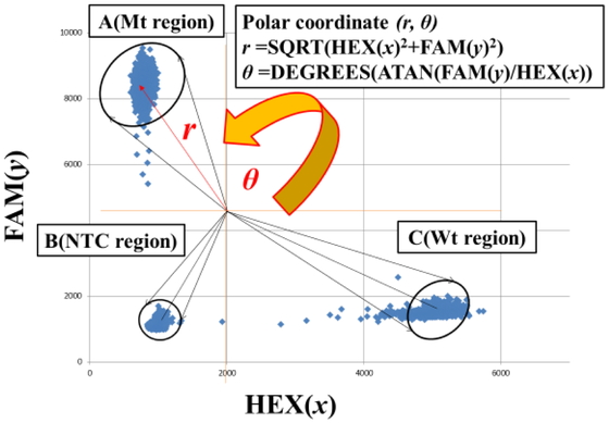
The origin (x = 0, y = 0) in two
dimensional orthogonal coordinate (x, y)
was moved to the gravity of A (Mt region), B (NTC region) and C (Wt region), and then, two
dimensional orthogonal coordinate (x, y)
were converted to two dimensional polar coordinate (r,
θ) (Figure 4). In
the two dimensional polar coordinate (r,
θ), all plots are observed by (θ)
histogram without any overlapping (Figure 5).
The gravity was obtained by cluster analysis method of three elements
(k = 3), such as A (Mt region), B (NTC region) and C (Wt
region). The gravity calculation was executed automatically by EXCEL Macro [7] for k-means clustering
method [8,9,10], a typical dividing-optimization
method. The explanation for conversion equation from two dimensional orthogonal coordinate
(x, y) to two dimensional polar
coordinate (r, θ) is described in Appendix
A (Conversion from two dimensional orthogonal coordinate (x,
y) to two dimensional polar coordinate
(r, θ)) and the consideration for angle
setting in converting to two dimensional polar coordinate (r,
θ) is described in Appendix B (Consideration for the angle
setting (0°– 360°) in converting from two dimensional orthogonal coordinate
(x, y) to two dimensional polar
coordinate (r, θ)), an example of EXCEL
Macro for the conversion is described in Appendix C (Conversion from two dimensional
orthogonal coordinate (x, y) to two
dimensional polar coordinate (r, θ) by
EXCEL Macro), respectively.
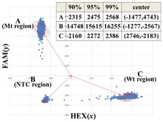
After the coordinate converting, the number of fluorescent signal plots in the A (Mt
region), B (NTC region) and C (Wt region) are calculated automatically using the normal
distribution probability density function “NORMDIST” in EXCEL at each of 90%, 95% and 99%
confidence interval, the gene mutation is determined by existence of fluorescent signal
plots in the Mt region, and the gene mutation rate is calculated by Mt fluorescent signal
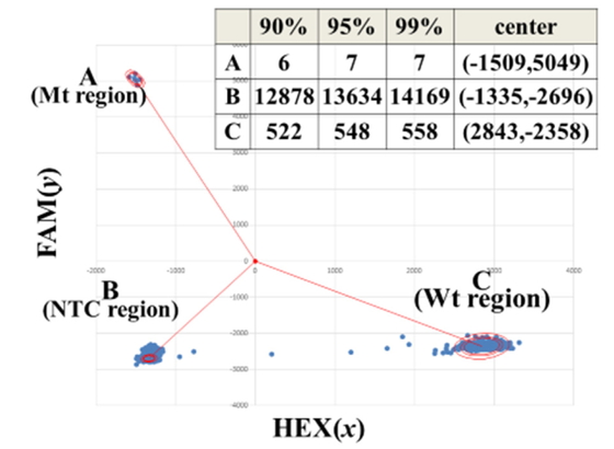
plots/(Mt fluorescent signal plots + Wt fluorescent signal plots). In Figure 6, the EXCEL Macro program execution result of ALK wild
type/resistant mutation type (L1196M) DNA (10,000copies) is shown, and in Figure 7, the EXCEL Macro program execution result
of ALK wild type/resistant mutation type (L1196M) DNA (Mt/Wt;10/1,000 copies) is shown
respectively.
2.4 EXCEL Macro Processing Procedure
It is possible to judge promptly and easily whether target gene mutations are present by
visualizing genetic analysis fluorescent signal plots data through the following
processing procedure of EXCEL VBA MACROS analysis except that the Steps 1) and 9) were
input and evaluated manually.
[Operating Procedure]
1) Data uptake two dimensional orthogonal coordinate (x,
y)
2) Determine centroids for corresponding A (Mt region), B (NTC region) and C (Wt
region) by k-means clustering method
3) Determine the gravity point of triangle formed by the centroids for A (Mt region), B
(NTC region) and C (Wt region)
4) Parallel move of the origin of two dimensional orthogonal coordinate
(x, y) to the gravity point
5) Conversion to two dimensional polar coordinate (r,
θ)*
* r=SQRT (X^2+Y^2), θ
=DEGREES (ATAN (Y/X))
6) Histogram preparation based on (θ) degrees
7) Calculate the number of fluorescent signal plots distributed in A (Mt region), B
(NTC region) and C (Wt region) within 90%, 95% and 99% confidence interval by NORMDIST
function
8) Re-conversion** to two dimensional orthogonal coordinate (x,
y) and elliptical graph of 90%, 95% and 99% confidence
interval display
** x=r*COS (RADIANS
(θ)),
y=r*SIN (RADIANS
(θ))
9) Determine gene mutation and calculate gene mutation rates within 90%, 95% and 99%
confidence interval, respectively
3 DISCUSSION
In quantitative analysis from histograms in HEX (x axis) and
FAM (y axis), it is difficult to show each distribution state
of the fluorescent signal plots in A (Mt region), B (NTC region) and C (Wt region) at the
same time, due to overlapping of fluorescent signal plots in A (Mt region) with those in B
(NTC region) or C (Wt region) with B (NTC region) so far. Therefore, the origin
(x = 0, y = 0) was moved to the gravity
point inside of the triangle consisting of A (Mt region), B (NTC region) and C (Wt region),
and the two dimensional orthogonal coordinate (x,
y) were converted to the two dimensional polar coordinate
(r, θ). It is confirmed that this
approach made it possible to show separately all fluorescent signal plots of the three
regions such as A (Mt region), B (NTC region) and C (Wt region) in histogram at one time
without any overlapping and easy to count the number of fluorescent signal plots in A (Mt
region) and C (Wt region). Furthermore, we consider that employing an automated processing
from coordinate conversion to graphic visualization of results by EXCEL Macro is useful for
identifying mutation occurrence and mutation rate promptly. For the future, we are hoping to
develop a more convenient genetic analysis method by processing more samples using the
method described here.
REFERENCES
- [1] X. Shi, C. Tang, W. Wang, D.
Zhou, Z. Lu, Electrophoresis, 31, 528 (2010). ,
doi:10.1002/elps.20090036220119960
- [2] E. A. Ottesen, J. W. Hong,
S. R. Quake, J. R. Leadbetter, Science, 314, 1464 (2006). ,
doi:10.1126/science.113137017138901
- [3] B. Vogelstein, K. W.
Kinzler, Proc. Natl. Acad. Sci. USA, 96, 9236 (1999). ,
doi:10.1073/pnas.96.16.923610430926
- [4] S. Dube, J. Qin, R.
Ramakrishnan, PLoS One, 3, e2876 (2008). ,
doi:10.1371/journal.pone.000287618682853
- [5] B. J. Hindson, K. D. Ness,
D. A. Masquelier, P. Belgrader, N. J. Heredia, A. J. Makarewicz, I. J. Bright, M. Y.
Lucero, A. L. Hiddessen, T. C. Legler, T. K. Kitano, M. R. Hodel, J. F. Petersen, P. W.
Wyatt, E. R. Steenblock, P. H. Shah, L. J. Bousse, C. B. Troup, J. C. Mellen, D. K.
Wittmann, N. G. Erndt, T. H. Cauley, R. T. Koehler, A. P. So, S. Dube, K. A. Rose, L.
Montesclaros, S. Wang, D. P. Stumbo, S. P. Hodges, S. Romine, F. P. Milanovich, H. E.
White, J. F. Regan, G. A. Karlin-Neumann, C. M. Hindson, S. Saxonov, B. W. Colston, Anal.
Chem., 83, 8604 (2011). , doi:10.1021/ac202028g22035192
- [6]Kyoritsu Sugakukosiki,
Kyoritsu Shuppan, pp. 111 (1975)
- [7] S. Neilson, “k-Means Cluster
Analysis in Microsoft Excel” (2011).
http://www.neilson.co.za/k-means-cluster-analysis-in-microsoft-excel/
- [8] H. Steinhaus, (French).
Bull. Acad. Polon. Sci., 4, 801 (1957).
- [9] E. W. Forgy, Biometrics, 21,
768 (1965).
- [10] J. B. MacQueen, “Proceedings of
5-th Berkeley Symposium on Mathematical Statistics and Probability”, Berkeley, University
of California Press, 1, 281–297 (1967).