The o2o3 Local Galerkin Method Using a Differentiable Flux Representation

Abstract

The spectral element (SE) and local Galerkin (LG) methods may be regarded as variants and generalizations of the classic Galerkin approach. In this study, the second-order spectral element (SE2) method is compared with the alternative LG scheme referred to as o2o3, which combines a second-order field representation (o2) with a third-order representation of the flux (o3). The full name of o2o3 is o2o3C⁰C¹, where the continuous basis functions in C⁰-space are used for the field representation and the piecewise third-order differentiable basis functions in C¹-space are used for the flux approximation. The flux in o2o3 is approximated by a piecewise polynomial function that is both continuous and differentiable, contrary to several Galerkin and LG schemes that use either continuous or discontinuous basis functions for flux approximations. We show that o2o3 not only has some advantages of SE schemes but also possesses third-order accuracy similar to o3o3 and SE3, while SE2 possesses second-order accuracy and does not show superconvergence. SE3 has an approximation order greater than or equal to three and uses the irregular Gauss-Lobatto collocation grid, whereas SE2 and o2o3 have a regular collocation grid; this constitutes an advantage for physical parameterizations and follow-up models, such as chemistry or solid-earth models. Furthermore, o2o3 has the technical simplicity of SE2. The common features (accuracy, convergence, and numerical dispersion relations) and differences between these schemes are described in detail for one-dimensional homogeneous advection tests. A two-dimensional test for cut cells indicates the suitability of o2o3 for realistic applications.

1. Introduction

Some numerical atmospheric models use the classic Galerkin method or its variants to discretize the state variables of the atmospheric motion equations in basis functions. The global spectral method (Simmons et al. 1989) uses spherical harmonic basis functions, whereas the finite element (FE) method applies the classic Galerkin method in combination with local basis functions (Steppeler 1987). The advantages of the classic Galerkin FE method include the combination of a high approximation order (third or fourth order) with conservation properties and its suitability for irregular grid structures. Another advantage, namely, a sparse grid, is obtained when the Galerkin method is combined with higher than first-order FEs; in other words, some of the points in the regular grid are omitted, considerably reducing the computational time. For the FE method, such sparse grids are called serendipity grids (Ahlberg et al. 1967).

Classic Galerkin methods involve the solution of a linear equation related to the mass matrix. When the matrices are solved by direct methods, such as Gaussian elimination (Steppeler et al. 1990), they require global communication, although the basis functions are local and the mass matrix has a band structure. As classic FE methods require global communication between all cells within the computational domain, it is difficult to scale such models for very large numbers of processors. Accordingly, variants of the classic Galerkin procedure known as local Galerkin (LG) methods were developed (Steppeler and Klemp 2017). Particularly, spectral element (SE) techniques are LG methods that have undergone substantial development and are almost suitable for operational use (Herrington et al. 2019). SE methods have achieved scalability for the Nonhydrostatic Unified Model of the Atmosphere for up to millions of processors (Taylor et al. 1997; Giraldo 2001; Giraldo and Rosmond 2004; Kelly and Giraldo 2012). The present paper investigates a higher-order LG method referred to as o2o3, the full name of which is o2o3C⁰C¹. The continuous basis functions for the field representation are piecewise quadratic polynomials in C⁰-space, while third-order differentiable basis functions in C¹-space are used for the flux approximation. o2o3C⁰C¹ is a further development of the o3o3C⁰C⁰ method (Steppeler et al. 2019a). Both o2o3 and o3o3 can be considered variants and generalizations of the SE technique. High-order SE methods use the irregular Gauss–Lobatto grid, possibly limiting the time step. Steppeler et al. (2019a) demonstrated that o3o3 inherits the advantages of SEs and allows a larger time step to improve the computational efficiency. Although the effective resolution of o3o3 as defined by Ullrich et al. (2018) is comparable with that of the third-order spectral element method (referred to as SE3), a dispersion analysis showed that o3o3 has a large 0-space. This means that waves are stationary for a relatively large range of wavenumbers.

Classic Galerkin approaches are widely applied in computational fluid dynamics, where irregular cells are used to correctly describe the surface of an airplane. In a meteorological context, this property may translate into an accurate representation of the lower surface, meaning a more accurate approximation of mountains. Additionally, FEs are expected to improve the impact of mountains on atmospheric circulation. For meteorological models, it is important for the lines composed of grid points to be horizontally aligned (Steppeler et al. 2006). Hence, these horizontal lines of grid points cut into the mountains. However, the lower boundary representation is complex, which hinders the use of this approach during the modeling process. Terrain-following coordinates enable the alignment of the grids with the surface topography, thereby simplifying the computation of the lower boundary condition (Phillips 1957). Horizontally aligned grids are normally constructed using a regular height grid structure where only the surface grid cells are irregular (Yamazaki and Satomura 2010). The horizontal alignment of numerical grids and the underlying terrain, such as that obtained with cut cells (Nishikawa and Satoh 2016), will result in a more accurate representation of mountains (Steppeler et al. 2006; Zängl 2012). Steppeler et al. (2019b) showed that cut cells provide a better representation of vertical velocities in a three-dimensional realistic model than the models using terrain-following coordinates, leading to improved forecasts. Consequently, cut-cell models were used with grid point numerical methods (Yamazaki et al. 2016; Steppeler et al. 2019b).

Steppeler and Klemp (2017) showed that some finite-difference (FD) cut-cell approximations can produce noisy solutions even for smooth mountains. Their work was limited to linear test functions and a rather simple test mountain consisting of a straight line. However, SE and FE methods are mostly performed on grids that are not horizontally aligned (Marras et al. 2016). The advantages of cut cells in representing mountains proposed by Steppeler and Klemp (2017) are not realized with these FE/SE representations. By contrast, Galerkin methods using first-order basis functions and horizontally aligned grids lead to solutions without such noise (Steppeler and Klemp 2017). This finding confirms the fact that Galerkin methods lead to accurate surface approximations when the cells are adapted to the surface, that is, for horizontally aligned cells. Nevertheless, existing atmospheric Galerkin models often do not take advantage of such suitability for good surface approximations because grids that are not horizontally aligned are typically used. A notable exception is the atmospheric model called Active Tracer High-resolution Atmospheric Model-Fluidity (ATHAM-Fluidity) that uses horizontally aligned cells and achieves good results in the generation of mountain-induced waves (Savre et al. 2016).

In this study, we construct o2o3 to address the disadvantages of o3o3, and we demonstrate the following properties of o2o3:

• ・The accuracy of o2o3 is comparable with that of SE3 as a result of the constructed superconvergence, although o2o3 has the simplicity and basis function structure of the second-order spectral element method (referred to as SE2).
• ・o2o3 uses a regular collocation grid, whereas SE3 uses the irregular Gauss–Lobatto grid; the former is an advantage when parameterizing physical processes (Herrington et al. 2019).
• ・A sparse grid is possible with o2o3, whereas SE3 uses a full grid.
• ・o2o3 avoids the large 0-space of o3o3.
• ・The suitability of the high-order o2o3 method for cut cells is shown using the simple example of Steppeler and Klemp (2017). Therefore, o2o3 allows for cut-cell implementation in second- and third-order spaces, whereas the Steppeler and Klemp (2017) scheme uses linear basis functions.

We describe the grid and approximation spaces for SE2, o2o3, and SE3 in Section 2. A summary of the numerical properties of all schemes compared in this paper is given in Table 1. Section 3 outlines the inhomogeneous FD schemes representing the approximations of these schemes. Section 4 presents the LG procedure for o2o3, conserving first-order moments. Section 5 illustrates the results of a homogeneous advection test to show the accuracy and stability, convergence and numerical dispersion relations of o2o3, and the study is concluded in Section 6.

2. Grids and approximation spaces

In this study, the test problem involves homogeneous one-dimensional (1D) advection of the density field h(x):   

where u₀ is the velocity field, assumed to be constant, and the periodic boundary condition is imposed.

Equation (1) is solved using piecewise polynomial spaces of degrees 2 and 3. These are the discretization spaces used with the continuous Galerkin schemes o2o3, SE2, and SE3. Let a 1D domain Ω be divided into the elements Ω_i (i = 0, 1, 2, …), where Ω_i = (x_i, x_i+1). In each element Ω_i, the polynomial P_i (x) = is determined by three polynomial coefficients p_i,0, p_i,1, p_i,2 for SE2 and by four coefficients p_i,0, p_i,1, p_i,2, p_i,3 for SE3. The index i indicates that the polynomial representation is applicable to the element Ω_i. Hence, for a discontinuous second-order field representation, the polynomial coefficients p_i,0, p_i,1, and p_i,2 are independently chosen and are the degrees of freedom. The spaces formed by p_i,0, p_i,1, p_i,2, and p_i,3 are used for third-order discontinuous and continuous field representations. For the continuous Galerkin scheme, the polynomials must fit together continuously, implying the condition P_i−1 (x_i) = P_i (x_i) and P_i (x_i+1) = P_i+1 (x_i+1). Therefore, we have only two degrees of freedom per element with SE2 and three for SE3.

In one dimension, the length of the element Ω_i is defined as dx_i = x_i+1 − x_i. If the grid distribution is regular, then dx = dx_i. The boundary grid points x_i and x_i+1 of the element Ω_i are called the principal points or corner points. For SE2, there are three independent amplitudes described by three collocation point values in each element, whereas there are four amplitudes for SE3 (Fig. 1). Collocation points are grid points within an element such that the amplitudes at these points are sufficient to determine the polynomial coefficients corresponding to this element. For SE2 and o2o3, the fields are quadratic polynomials within the element Ω_i, and we need three collocation points X_i,0, X_i,1, and X_i,2. Although we have three collocation points per element, the dimension of the collocation grid space is twice as large as the number of elements, as principal points are shared by two elements. For a third-order field representation, such as with SE3 or the flux for o2o3, we need two interior points besides two principal points. Hence, the collocation grid points are X_i,j (i = 0, 1, 2, …, j = 0, 1, …, J) in Ω_i:   

where x^m_i = ½(x_i + x_i+1 is the midpoint of the element Ω_i. We have J = 2 for o2o3 and SE2 and J = 3 for SE3. The collocation grids X are noted by broken indices: x_i+1/2 = X_i,1 for SE2 and o2o3 and x_i+1/3 = X_i,1, x_i+2/3 = X_i,2 for SE3. We note that in Eq. (2), the collocation points form a set of Gauss–Lobatto points of either three (SE2 or o2o3) or four (SE3) nodes. The sets of points are redundant as follows:   

Fig. 1.

Grids for o2o3, SE2, and SE3, in which the solid black points represent the principal nodes and the dashed white points represent the interior nodes of the elements.

The field values at collocation points form the grid point space. The points X_{i, j} must be used to derive the initial data for the three schemes.

The basis functions used to define the field h (x) in Eq. (1) are the same among the three schemes. The basis functions are defined in the interval (x^m_i − ½dx_i, x^m_i + ½dx_i) as follows:   

These four basis functions are identically zero when .

For any field or flux q (x), we can derive the discretized representation using the basis functions defined in Eq. (4):   

where ε = 0 is used for the second-order field representation with SE2 and o2o3, whereas ε = 1 is used for the flux in the third-order representation with o2o3. For the representation of discontinuous functions, two values of q (x) at principal nodes are introduced: q_i⁺ and q_i⁻. We note that in this study, discontinuous functions occur for flux derivatives with SE2 and SE3. In Eq. (5), the amplitudes q_i, q_{xx, i+1/2} form the spectral space for SE2 and o2o3, whereas the amplitudes q_i, q_{xx, i+1/2}, q_{xxx, i+1/2} form the spectral space for SE3. For the field q (x), the grid point space for SE2 and o2o3 is formed by q_i and q_i+1/2 (i = 0, 1, 2, 3, …). According to Eq. (5), q_i at the principal nodes represents both the spectral amplitudes and the grid point values for the three schemes.

Using Eq. (5), we can obtain the transformation equations to the grid point space at the midpoints x_i+1/2 for SE2 and o2o3 with ε = 0:   

From Eq. (6), we can obtain the transformation from the grid point space to the spectral space in Ω_i. When q_i, q_i+1 and q_i+1/2 are given, the transformation to the spectral space is as follows:   

For the third-order space used in SE3, we refer to Steppeler et al. (2019a) for the formulas of the transformation between the grid point space and spectral space. A list of published LG schemes and their discretization spaces is given in Table 1.

We note that o2o3 for the two-dimensional (2D) problem is obtained by differencing along the coordinate lines, analogous to the 2D o3o3 scheme derived in Steppeler et al. (2019a). Thus, the 1D scheme is extracted while leaving the interior points out. Hence, the 2D grid becomes sparse for interior points that are not used for forecasting. This means that the sparse grid is obtained from the full grid (all points are dynamic) by removing the interior points, as illustrated in Fig. 2. Thus, only the grid points at the corners and edges are dynamic. Steppeler et al. (2019a) defined the sparseness factor as the ratio of the number of dynamic points to the number of points in the full grid. A small sparseness factor indicates the potential for reducing the computational time.

Fig. 2.

o2o3 computational grid in two dimensions: (a) full grid and (b) sparse grid where unused points are shown in white.

3. Inhomogeneous finite difference schemes

The classic fourth-order FD scheme (o4) is a homogeneous FD scheme that uses the same FD formula at each grid point. By contrast, SE and other LG schemes typically use different discretization equations at each collocation point (Steppeler et al. 2019a); these approaches are known as an inhomogeneous FD scheme. In this section, we discuss inhomogeneous FD schemes resulting in the temporal derivatives of the field q (x) for a regular grid distribution dx_i = dx.

SE2, o2o3, and SE3 are used as examples for comparison. For all three examples, q (x) within the cells is approximated by polynomials. For any of the collocation points, these polynomials are not centered around the target point (the point to compute the derivatives). Instead, to obtain the spatial derivative of q (x) in a cell, the polynomial is differentiated at different collocation points. We note that the right and left derivatives (q⁺_{x, i} and q⁻_{x, i}) at the principal points are defined discontinuously between two different cells; hence, an averaging procedure for q⁺_x,i and q⁻_x,i must be defined to obtain q_x,i. Thus, the FD schemes in a cell differ among the collocation points, and consequently, the three schemes are inhomogeneous in the grid point space. In the following paragraphs, we introduce three schemes for both principal and interior points except that o2o3 for the interior points will be defined in the next section.

For SE2, the time derivative in Eq. (1) at the collocation points can be computed using the field representation Eq. (5) with ε = 0. For the interior points in Ω_i, the functional representation in Eq. (5) is differentiable, and we can obtain the following:   

where b²_x,i (x_i^m) = 0.

For the principal points x_i in Ω_i, the basis function in Eq. (4) has a discontinuous derivative, and we obtain the right and left derivatives, q⁺_x,i and q⁻_x,i at x_i from Eq. (5). These values are obtained as follows:   

where we use the transformation formula for the spectral space and Eqs. (4), (5), and (7).

If the derivative at a principal node is defined as the average of these two values, we can write q_t,i as follows:   

The right-hand-side term in Eq. (10) is a linear combination of two centered FD schemes with second-order accuracy. By comparing Eq. (8) with Eq. (10), this scheme can be recognized as an inhomogeneous FD scheme. Because neither Eq. (8) nor Eq. (10) has an approximation order higher than two, superconvergence does not occur for SE2.

o2o3 may be viewed as a generalization of SE2 with constructed inherent superconvergence to an order of at least three. Thus, o2o3 will be introduced as an inhomogeneous FD scheme. For the principal grid points in Ω_i, any FD scheme of at least the third order may be chosen. Here, we choose the classic o4 scheme:   

for the derivatives at the principal nodes in Ω_i.

Equation (11) guarantees fourth-order accuracy at corner points on regular grids (Durran 2010). However, for irregular grids, the accuracy drops to the first order. Now, we list the formula for calculating q_t on an irregular grid. When we apply Eq. (11) for all points, the rather strong deviation from conservation occurs partly because of a decrease in the order of approximation to 1. This decrease in the order of approximation is then counteracted by smoothly changing the resolution. Grid smoothing methods, such as “spring dynamics” (Tomita et al. 2001), are applied, whereas the Voronoi type of smoothed grid is used for the Model for Prediction Across Scales (Skamarock et al. 2012). For irregular grid structures, an alternative generalized formulation of Eq. (11) is derived as follows (Steppeler et al. 2008):   

where the corresponding weights w_i shown in Table 2 are computed numerically, for example, by polynomial fitting in Steppeler et al. (2019a). A simplification is achieved by replacing the Legendre representation of the polynomial space with order-consistent polynomials. Any other high-order FD scheme can be used as an alternative to Eq. (11) or Eq. (12). In the following text, we refer to the o4 scheme given by Eq. (11) as classic o4, whereas the o4 scheme given by Eq. (12) is referred to as weighted o4. We consider an example of irregular grids as defined in the seventh column of Table 2 (see also Section 5.1). With these weights, a third-order approximation can be achieved when we apply the differentiation to analytic test functions, such as polynomials of degree 3. We note that the value of w_i in the fine mesh area (dx = 1) is twice the value in the coarse mesh area (dx = 2). The advantages of Eq. (12) will be demonstrated in Section 5.1.

For comparison purposes, we also use SE3. For the principal nodes in SE3, averaging between right and left values, as performed in Eq. (10), is adapted to the third-order representation. For the two interior nodes, Eq. (8) is used analogously because the basis function representation for SE3 is directly differentiated.

Finally, the proof of the third-order approximation of Eq. (11) follows from the requirement of third-order consistency. The FD equation for mass follows directly from Eq. (5). Let dm_i be the mass contained in the element Ω_i = (x_i, x_i+1):   

Then, we have:   

The mass conservation property requires that the time derivative of the mass of dm_i within the element Ω_i is the flux difference at the two principal points of the element Ω_i. We show this in the next section.

4. Local Galerkin procedure

In this section, with the field representation defined in Section 2, we introduce the LG procedure to define o2o3 in comparison with SE2 and SE3.

We assume h (x) to be represented in the grid point space by h_i, and we assume that h (x) can be transformed into the spectral space by Eq. (7). This will result in the spectral amplitudes h_i and h_xx,i+1/2 for SE2 and o2o3 and the spectral amplitudes h_i, h_xx,i+1/2 and h_xxx,i+1/2 for SE3 in Ω_i. Using these amplitudes, Eq. (5) gives the functional form of h (x).

For SE2 and SE3, fl (x) = −u₀h(x) can be defined using the representations in Eqs. (5) and (7). For SE2, we have the following:   

For SE3, we refer to Eqs. (5) and (7) analogously:   

We note that in this study, discontinuous functions occur for flux derivatives with SE2 and SE3.

To define o2o3, the temporal derivative of the field is proportional to the spatial derivative according to Eq. (1), which means that we only need to determine the expressions of h_t,i = fl_x,i at the principal nodes and of fl_xx,i+1/2 and fl_xxx,i+1/2 at the interior nodes within Ω_i. However, in o2o3, the field h (x) given by Eq. (5) has only a second-order representation. Thus, we apply Eq. (5) with ε = 1 to define a third-order representation of the flux fl (x).

At the principal nodes in Ω_i with o2o3, we again define the following:   

which will not be used, as we are interested only in the flux divergence used in Eq. (1), rather than in the value of the flux itself. The third-order flux representation according to Eq. (11) is defined such that fl (x) is differentiable at the principal nodes of Ω_i . The degree-3 polynomial is defined such that the derivatives at the principal points have the same value for left and right differentiation. Thus, by construction, we obtain a differentiable spline. The derivative fl_x,i at the principal nodes of fl (x) is defined analogously to Eq. (11) up to a classic o4 approximation:   

We note that the definition in Eq. (18) already gives the FD equations at the principal nodes according to Eq. (1):   

At the interior points within the element Ω_i, the values of fl_xx,i+1/2 and fl_xxx,i+1/2 follow the continuity requirement of the functional representation in Eq. (11) at the principal nodes [see the details of the steps to derive the time derivative of h (x) in Fig. 3]. We provide two methods to obtain the expressions of fl_xx,i+1/2 and fl_xxx,i+1/2.

Fig. 3.

Approximations of the flux and the flux derivative of the field h(x) by the (a) SE2, (b) o2o3. and (c) SE3 schemes. The solid curves are the field h(x), and the dashed curves are the flux. The dotted curves represent the derivative of the flux, whereas the blue curves represent the regularized derivative, which is the derivative approximated by a continuous function. The regularized derivative is applied with SE2 and SE3. The grid intervals are shown corresponding to the dotted curves, where the long vertical lines represent the principal points and the short vertical lines are the interior points. In (a) and (c), the flux is different from h(x) only by the factor −1. In (b), the flux fl(x) is approximated by a differentiable function, and the flux derivative does not need to be regularized, as fl(x) is differentiable. In (c), h(x) is a third-order representation.

In the first method, the equations for the spectral coefficients fl_xx,i+1/2 and fl_xxx,i+1/2 are obtained by taking the x-derivative of Eq. (5):   

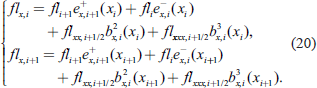Equation (20) is an equation for fl_xx,i+1/2 and fl_xxx,i+1/2, as all other quantities are known. The derivatives of e⁺_i+1, e_i⁻, b_i² b_i³ are obtained from their definitions in Eq. (4). Using Eqs. (4), (5) and (20), we can derive the expressions for the spectral amplitudes at the interior points x_i+1/2:   

and   

For the time derivative at the interior point of an element, according to b³_x,i(x_i+1/2) = −1/24dx² and Eqs. (4), (5), (21), and (22), we can obtain the following:   

In the second method, we directly apply the principle of the conservation of mass to construct Eq. (23). Let the time derivative of h at the principal nodes be given again by Eq. (19) or by any other difference scheme of at least the third order. By differentiating Eq. (14) with respect to t, the time derivative of the mass dm_t,i in the element Ω_i is obtained as follows:   

dm_t,i can also be computed from the flux into Ω_i, and we obtain the following:   

By combining Eqs. (24) and (25) and solving for h_t,i+1/2, we obtain Eq. (23). These two methods lead to the same piecewise quadratic polynomial representation. The uniqueness of the two methods follows from the fact that the equation of motion is assumed to be valid with the spatial flux representation as a piece-wise cubic spline. The derivation of Eq. (23) from the basis function representation implies the conservation of first-order moments, corresponding to the conservation of mass in this case. Thus, Eqs. (23) and (18) can be viewed as a method for defining the time derivative h_t,i such that mass is conserved.

Figure 3 illustrates the steps for the computation of the time derivative of the field h. The field is defined as h (x_i) = 0, except for h (x₅₀₀) = 4. This defines a rather small-scale field for which different numerical methods are expected to give different results. For smooth fields, all methods must give very similar results. Figure. 3a shows the results with SE2. The flux in this case that is shown as the dashed curve is merely the negative of the field. However, the spatial derivative of the flux shown by the dotted line, is discontinuous. The blue curve is the result of the LG operation that approximates the derivative by a continuous function. Figure 3b shows similar results for o2o3. The flux shown by the dashed curve is approximated by a differentiable function, and the spatial derivative of the flux shown by the dotted curve is continuous; thus, no further approximation is necessary. Figure 3c gives the result for SE3, which is analogous to the result shown in Fig. 3a, but with the approximating polynomial of degree 3. We note that the grid is different from that of SE2 because its length is 3dx

For all of the described methods, when the time derivative h_t(x) is given in the grid point space, the fourth-order Runge–Kutta method (RK4) can be applied as with any other FD scheme. Although the example of Fig. 3 uses a low resolution, all methods give a reasonable approximation of the time derivative. This is important, since practical calculations in meteorology depend on reasonable approximations with poor resolution in some instances (Steppeler et al. 2003), and the orography is often not well-resolved in atmospheric models.

Thus far, we have already illustrated how to generate the inhomogeneous o2o3 scheme for h_t,i and h_t,i+1/2 using the homogeneous 1D advection equation Eq. (1). Overall, the steps of the implementation of o2o3 are described as follows:

• ・Step 1: Divide the computational domain (Fig. 1) into elements and define the collocation points Eq. (2) in each element. Note that the collocation points include the corner point and interior point for o2o3;
• ・Step 2: Define the basis functions Eq. (4) for the field representation and flux representation Eq. (5) in each element;
• ・Step 3: Construct the temporal derivative of field h_t,i Eq. (19) at corner points by Eqs. (1) and (17) and a classic o4 scheme Eq. (18);
• ・Step 4: Construct the temporal derivative of field h_t,i+1/2 at interior points by Eq. (23) or the condition of flux conservation expressed by Eqs. (24) and (25). Note that to achieve the variable h_t,i+1/2, we must rely on the intermediate variables: the second- and third-spatial derivatives of the flux at the interiror point expressed by Eqs. (21) and (22);
• ・Step 5: Compute h_i and h_i+1/2 at the next time level using the RK4 method or any proper time integration scheme.

Note that the time loop consists of Steps 3, 4, and 5. Steps 1 and 2 are used to initialize the forecast.

5. Results

To investigate the characteristics of o2o3, including its accuracy, convergence, numerical dispersion and stability, homogeneous advection tests in both one and two dimensions are implemented. For a first examination of the suitability of o2o3 for high-order cut-cell modelling, an advection test along a straight mountain is implemented.

5.1 1D homogeneous advection test

The advection equation in Eq. (1) is solved for a 1D area with 600 points, and the constant-velocity field u₀ is set to be u₀ = 1.0. For o2o3 and SE2, 300 elements are present in the area, whereas for SE3, 200 elements are present.

With an element length dx = 2 for o2o3 and SE2, the resolution of the collocation grid is dx^r = 1. Table 3 shows the Courant–Friedrichs–Lewy (CFL) condition with RK4 time-stepping. The available time steps (i.e., CFL condition) are 2.2, 1.8, and 1.5 for SE2, o2o3, and SE3, respectively. According to conventional wisdom (Durran 2010), classic o4 has a stability limit of 1.9 with the RK4 scheme. This means that o2o3 has a marginally smaller CFL condition than the classic o4 scheme. The relatively weak CFL condition with SE3 can be explained by the minimum grid size of the Gauss–Lobatto grid being lower than that of the equally spaced grid used with o2o3. Thus, the time step in o2o3 is approximately 20 % higher than that in SE3. However, these two schemes are comparable in terms of their accuracy and conservation properties. The large CFL number of SE2 is to be expected, given that the transition to a higher order often requires a smaller time step. Ultimately, the CFL conditions for o2o3, SE2, and SE3 are more severe than those for the second-order centered FD scheme.

To measure stability, we perform temporal integration for a long time. We use 30000/dt steps, meaning that the structure is transported over 30000 grid points or 15000 elements over the area. Because of the periodic boundary conditions, for t = 600 n (n = 1, 2, 3, …), the analytic solution of Eq. (1) is identical to the initial value, so that the accuracy can easily be checked at these times.

Figure 4 shows the solutions of the homogeneous advection test after transport over 300dx and 30000dx. The initial value of h(x) is defined as follows:   

The results for SE2, o2o3, and SE3 are shown in the left, middle, and right columns of Fig. 4, respectively. At 300 time steps, the results for the three schemes are similar except for a slight oscillation in SE2. At the 30000th timestep, SE3 and o2o3 show a better simulation quality than SE2 because SE2 is only of the second order. The small difference in the accuracy between o2o3 and SE3 is in accordance with the results of the numerical dispersion analysis in Section 5.3. For an analysis of the order of approximation, see Section 5.2.

Fig. 4.

Solutions of the homogeneous advection equation with periodic boundary conditions after transport over 300dx and 30000dx, and the length of the horizontal area is 600dx. The initial condition centered at 150dx is shown in (a). The second row shows the results after transport over 300dx, whereas the third row shows the results after transport over 30000dx. The left, middle, and right columns are the results with SE2, o2o3 and SE3, respectively. Because of dx = dt = 1, the transport of 30000dx is done in 30000dt. This value of dt means that all schemes perform well in their CFL limit.

For the regular resolution case and periodic boundary conditions, both classic o4 and o2o3 are conserving. However, a lack of conservation will be observed only for o4 on irregular grids in practical tests. Hence, an irregular resolution is introduced:   

For o2o3, the weights w_i occurring in Eq. (12) are given in Table 2. The values of the weights gradually change near i = 180 (Lines 3–5 compared with Line 2 in Table 2) and 210 (Lines 7–9 compared with Line 10 in Table 2). All points x_i, where i ≠ 179, 180, 181, 209, 210, 211 according to Eq. (27), have constant w_i^i′ (i′ = −1, −½, 0, ½, 1) in Eq. (12), meaning that w does not depend on i. Figure 5 shows the temporal evolution of the solution between t = 0 and t = 400. For the initial values, the peak solution is used where only one principal point (x₁₅₀ = 4) is different from 0. The computational modes of both classic and weighted o4 are stronger than that of o2o3, particularly for the case of an irregular grid. Considering Steppeler et al. (2008) and Steppeler et al. (2019a), it may be assumed that the difference is due to the different orders of approximation at these points, where the resolution is irregular. Classic o4 decreases to the first order at such points. This is consistent with the fact that SE schemes are suitable for an irregular resolution, which (for this simple case) also applies to o2o3.

Fig. 5.

Solution of a single cell peak for the (a) classic o4 scheme with a regular cell structure, (b) weighted o4 scheme with an irregular cell structure, (c) o2o3 scheme with a regular cell structure, and (d) o2o3 scheme with an irregular cell structure. The black curves are the initial field and the forecasts at t = 100, 200, 300, and 400, and the red and blue curves are the forecasts at t = 30 and t = 60 at the start and end of the resolution jumps.

Mass diagrams of the solutions, defined as ∫_Ωh (x) dx, are shown in Fig. 6. The formula for computing the mass is given in Eq. (13). o2o3 conserves the mass down to the round-off error, whereas o4 conserves the mass until the resolution jump is reached. Then, the deviation from conservation is rather strong (reaching 50 %) and diminishes for advection in the coarseresolution area.

Fig. 6.

Mass diagrams for the (a) classic o4 scheme with a regular cell structure, (b) weighted o4 scheme with an irregular cell structure, (c) o2o3 scheme with a regular cell structure, and (d) o2o3 scheme with an irregular cell structure. With the nonconserving o4 scheme, deviations of mass conservation occur when the advected structure reaches the lower-resolution area and to a smaller degree when the highly resolved area is reached again.

5.2 Comparison of the convergence of o2o3 with that of o3o3 and SE

This section investigates the approximation order of the schemes considered in this paper. Because a general function can be approximated by a Fourier transformation of the sum of trigonometric functions, we investigate the accuracy of the approximation of the derivative of a cosine function g(x) that can be expressed as follows:   

We assume a grid distribution as follows:   

where r_i is a fixed random number between zero and one. When the grid is regular we set δ = 0. When the grid is irregular, δ is any positive real number between 0 and 1. For δ > 0.0, we obtain the irregular case, and in this case, we set δ = 1.0. Using the grid point values g_i = g(x_i) and using the grid approximations described in Sections 3 and 4, the approximations g^app_x,i at x_i can be obtained. The corresponding exact values g_x,i = −2π · sin (2πx_i) can be used to find the approximation error as follows:   

Figure 7 shows the numerical errors of its spatial derivative with dx = ⅛, ¼, ½, 1, 2, 4, 8, 16, 32, and 64. The classic o4 scheme converges to the fourth order only on regular grids. For comparison, the result for SE2 on regular grids is shown to exhibit second-order convergence, meaning that there is no superconvergence for SE2. By contrast, the high-order flux computations with o2o3 lead to superconvergence.

Fig. 7.

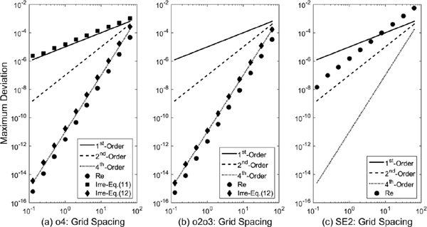
Convergence speeds of o4, o2o3, and SE2 under irregular and regular grids for different grid spacings: dx = ⅛, ¼, ½, 1, 2, 4, 8, 16, 32, and 64. The left, middle and right panels are the results for o4, o2o3 and SE2, respectively. The circles represent the error norms for a regular grid, where Eq. (11) is used for o4 and o2o3, whereas the squares represent the error norms for an irregular grid, where Eq. (11) is used for o4, and the rhombuses are the error norms for an irregular grid, where Eq. (12) is used for o4 and o2o3. The squares in the left panel are used for classic o4 according to Eq. (11), leading to a first-order scheme on an irregular grid.

Next, the convergence on an irregular grid is investigated. The grid is defined in Eq. (29) where δ = 1.0. o2o3 converges to the fourth order with an irregular grid. The use of weighted o4 to compute the differences on principal grids is essential. Conversely, the classic o4 scheme is reduced to the first order for the irregular grid.

5.3 Dispersion analysis of o2o3

To derive the numerical dispersion relation for o2o3, we use spectral solutions following Ullrich et al. (2018). The field h is assumed to be as follows:   

where and c and k are the phase velocity and nondimensional wavenumber, respectively. Then, we define the amplitudes in the spectral space. For each k, the linear relation between and for Eq. (1) is given by the following:   

where is the temporal derivative of and the matrix M^k depends on the wavenumber k. The exact solution should be linearly dependent on k due to the following:   

where x_j = j · dx and j = 0, 1, 2, ….

We assume that a^k₁ and a^k₂ are defined as the eigen-values of the matrix M^k. Thus, the imaginary components of a^k₁ and a^k₂ represent the frequency ω(k) of the wavenumber k, whereas the real components are the diffusivity. The phase velocity of the wavenumber k becomes .

The evolution matrix M^k is given by the following:   

where M^k is applied to the amplitudes and . The matrices M¹, M², M³, M⁴ are 2 × 2 matrices that are given by the following:   

  

  

  

where M^k_j1,j2 is the element of matrix M^k in row j₁ and column j₂ (we assume dx = 1 and u₀ = 1 for simplification).

For o2o3, Figs. 8a and 8b show the phase velocity and the deviation of the amplification factor from unity, respectively, as functions of the nondimensional wavenumber. For comparison, the corresponding results for SE3 and o3o3 are also given. In Fig. 8a, we focus on the maximum of the frequency curve because the corresponding wavelength is the resolution limit for each scheme. For o2o3 and SE3, the approximated phase velocities are accurate for wavelengths greater than 3dx, with o3o3 performing somewhat worse. For smaller wavelengths, the derivative of the frequency curve becomes negative, resulting in a negative group velocity. This means that for this range of wave-numbers, the solution is not useful in terms of the propagation of wave packets. Based on this criterion, the useful wavelength range for o2o3 is larger than that for o3o3 by approximately dx. Finally, as shown in Fig. 8b, the amplification factor is one for all three schemes, and thus, the schemes are all nondiffusive.

Fig. 8.

Dispersion relations for o2o3, SE3, and o3o3. (a) is the imaginary part and (b) is the deviation of the eigenvalues from one, which is a measure of the intrinsic diffusivity of the scheme. All three schemes are non-diffusive. The black circles mark the spectral gap for SE3, producing negative group velocities in an area where the neighboring wavenumber values indicate a well-resolved solution.

The part of the spectrum with negative group velocities should be filtered. Sometimes, a more elaborate definition of the essential resolution is used (Ullrich 2014). This is based on the realistically approximated part of the dispersion diagram that shows the frequency as a function of the wavenumber. We note that o2o3 does not have the large 0-space of o3o3. The 0-space is a space where waves are stationary for a relatively large number of wavenumber values. For o3o3, there exists a 0-space with wavenumber values where physical waves are not captured (Steppeler et al. 2019a). Therefore, o2o3 is simpler to execute than o3o3.

Although SE3 has a marginally larger useful wave-length range than o2o3, we note that the dispersion relation for SE3 shows a spectral gap, as indicated by black circles in Fig. 8a. A spectral gap is a small wiggle on the frequency curve leading to a small area of negative group velocities in an otherwise well-resolved k-area located around the wavelength 8dx in Fig. 8a. Because of this spectral gap of SE3, Steppeler et al. (2019a) concluded that o3o3 has performance advantages over SE3. By contrast, o2o3 and o3o3 do not have spectral gaps. The methods for reducing the effect of the spectral gap for SE3 by applying hyperdiffusion have been discussed in the literature (Ullrich et al. 2018). In the absence of a spectral gap, an estimate of the usefully resolved wavenumber k is the range of k up to the maximum.

5.4 Von Neumann stability analysis of o2o3 for finite dt

In this section, the 1D advection equation in Eq. (1) is used for the classic Von Neumann stability analysis of o2o3. The waveform solution Eq. (31) of the field h and the linear relation Eq. (32) between and are utilized for this analysis.

For RK4 time integration, the amplification factor G is given by the following:   

where E is the identity matrix and   

The amplification factor G for o2o3 is shown in Fig. 9. The resulting stability is achieved for CFL = 1.9, consistent with the values obtained in Section 5.1.

Fig. 9.

(a) Von Neumann analysis results for o2o3. (b) is the cross-section of (a) at the nondimensional wavenumber k = π.

5.5 Two-dimensional cut-cell results using a sparse grid

As stated in Section 2, o2o3 can be easily adapted for 2D advection over simple terrain. This method is completely analogous to the method in Steppeler et al. (2019a) and can be considered a generalization of the o1o1 scheme treated by Steppeler and Klemp (2017). For details regarding the calculation, the readers are referred to Steppeler et al. (2019a). Here, we give only a short description.

Following Steppeler and Klemp (2017), we conduct a 2D advection test along the profile of a mountain composed of a straight line oriented at an angle of 45°. This test problem is very simple; we assume that the velocity is parallel to this straight line, and the velocity components (u₀ and w₀) are constant (1, 1). Despite the extreme simplicity of this example, Steppeler and Klemp (2017) showed that noise can be generated along the orographic line. We can examine how this kind of noise can be avoided.

Figure 10 shows that the sparse grid is available in the same manner as for o3o3. However, there is a difference in the sparseness factor between o2o3 and o3o3. The sparseness factor is the ratio of the number of grid points in the sparse grid to that in the full grid. According to Steppeler et al. (2019a), o3o3 has a sparseness factor of 5/9, whereas o2o3 has a sparseness factor of ¾ (as illustrated in Fig. 2). Comparing the result of Fig. 10 with that of Steppeler et al. (2019a) with a sparse grid, we find that o2o3 has fewer unused points than o3o3. However, discussing this finding in terms of practical modeling and numerical computation reduction is beyond the scope of this paper.

Fig. 10.

Two-dimensional results of o2o3 with a cut-cell grid under a straight line representing the terrain. The tracer in the first row is above the terrain, whereas the tracer in the second row is advected along the terrain. The first column presents the initial values of the tracers and the advection results after 100 time steps. The second column shows magnified views of the field at the locations of the initial values. The third column shows magnified views of the forecast fields. (b) and (e) show a background comprising zero field values with clusters of higher values. These points are marked in white in Fig. 2b; as these points are unused for forecasting, they retain their initial values. (c) and (f) show a smooth structure representing the field. At some points corresponding to the points marked in white in Fig. 2b, there is a steep point valley assuming the value of 0. The contour interval is set to be 0.5.

We define the fluxes in the x- and z-directions as follows:   

The flux divergences in the x- and z-directions at the principal points are computed by classic o4 because the cut and uncut cells in this case are regular. However, Eq. (12) must not be invoked because it is suitable for irregular grids. Applying the principle of mass conservation according to Steppeler et al. (2019a) and the formula obtained in Section 3, we obtain the following:   

For Fl^x_z,i,k+1/2, the result is similar. For the divergence in the z-direction, the same procedure is followed using the z-coordinate lines. The spectral amplitudes Fl_xx,i+1/2,k and Fl_zz,i,k+1/2 are then uniquely determined by requiring mass conservation for the fluxes in the x- and z-directions, respectively.

For uncut cells, this procedure is straightforward and analogous to o3o3. For the cut cells, a coordinate along the surface line is introduced. For this specific test problem, the streamlines of advection are parallel to the surface line x = z such that there is no flux and no flux divergence in the direction perpendicular to the surface. Because the orography is diagonal to the model area, the principal points lie on the orographic line that can be treated by classic o4. No interpolation is necessary for orography to cut the cells diagonally.

To this line x = z, we assume a coordinate s in the diagonal line with . Therefore, Eq. (42) for s-axis takes the following form:   

in which because the flux is in the direction of the diagonal line. Additionally, the time derivatives for the principal points on the boundary are obtained by differentiating along the diagonal boundary. Instead of rectangles, cut-cell grids can be applied for rhombohedral grids, resulting in quadrilaterals with two angles not equal to . This will complicate the computation of mass contributions by the different amplitudes relative to the rectangular grid case used here. However, in more general cases, the principle of mass conservation is used in the same manner as with squares to determine the amplitudes of the time derivatives at the midpoints of the edges.

For the experimental setup, we use a square grid of 140 × 140 grid points with dx = dz = 1.0, and we perform temporal integration for 100 time steps with dt = 1.0. The results for o2o3 are shown in Fig. 10 and can be compared directly with those by Steppler and Klemp (2017). The inaccuracies and noise for this problem, as seen for some non-Galerkin treatments, are absent; o2o3 is able to advect a structure along a straight line without generating noise. This result is consistent with that for the first-order Galerkin approach and with that obtained by Savre et al. (2016), who reported fewer numerical boundary-related errors for the classic Galerkin method. These results indicate that cut cells may be applicable with polynomial representations higher than 1.

The cut-cell example shown above is a rather special case because it is valid only when the orography passes through the diagonal of cells. The more general case where the orography is any straight line can be treated with only little more effort. The computational domain comprises the points above the orography. As the orography is a straight line of direction (u₀, u₀), we define the flux as (u₀h, u₀h) where h is the density. This means that the flux has no component perpendicular to the orography at each point on the orography. We call this the pointwise boundary scheme. Another option not followed in this paper would be to use the less stringent condition that the integrals of the vertical flux components over segments of the orographic line are 0.

The orography is shown as a red line in Fig. 11a and as a green line in Fig. 11b. The diagonal computational domain above the red line (gray area in Fig. 11a) is notated as S_d whereas the nondiagonal domain above the green line (gray area in Fig. 11b) is correspondingly notated as S_nd. Near the nondiagonal boundary, we have cells with triangles or pentagons marked in green, while the cells are squares and triangles at the diagonal boundary in red. There is more than one way to define the field representations near the small boundary sections in triangles/pentagons, and we are seeking the simplest scheme. Note that a polynomial function defined in a part of a rectangular cell, such as the small cut-cell triangles/pentagons in Fig. 11b, can be uniquely extended to the whole cell. Therefore, it is possible to define fields in the area S_nd by adopting the same discretization (such as Eq. 43) in the larger area S_d and restrict the field values in S_nd. Therefore, we can further define the temporal scheme in S_nd to be the same as that in S_d because S_d and S_nd share the common area S_nd.

Fig. 11.

Different options for the cut-cell grid. (a) Special case of a straight orographic line going through the cell corners, as was used in the example of Fig. 10. All cut cells in this case are triangular marked with red colors. (b) A general case where the orography does not cut each cell diagonally. The thick solid and green lines mark the boundary approximation cells. The cut cells are triangles or pentagons shown in green. The physical domains are the gray areas marked with S_d in (a) and S_nd in (b). The mass of the system is the integral of the density over the area above the orography. The polynomial field representations for the fluxes and the density can be uniquely extended to the whole area of the boundary approximation cells.

Let us assume the mass M_S for the area S:   

in which S can be either S_d or S_nd. When we define the S_nd scheme to be the restriction of the S_d scheme to the smaller area, we must show that a closed system is obtained. This means that no mass is lost through the boundary of S_nd, indicating that the fluxes of the S_d scheme are parallel to the boundary of S_nd (green line in Fig. 11) and to the boundary of S_d (red dotted line in Fig. 11). We can apply Stokes theorem to Eq. (1). For the time derivative of M_Snd, we obtain the following:   

in which Fl^⊥ is the flux component orthogonal to the boundary of S_nd in Fig. 11b. Thus, according to the scheme adopted in the area S_d, the mass is also conserved in S_nd due to the absence of flux components perpendicular to the green line. For convenience, we can define phantom amplitude points for the cut cells outside the computational domain and perform FDs for the area above the dotted line in Fig. 11b.

The case of cut cells with a curved boundary is beyond the scope of this paper. The derivations of Eqs. (44) and (45) use the pointwise cancellation of the flux at the boundary, which follows from the assumption of a constant velocity. However, the extension of fields and fluxes beyond the small triangles and pentagons can also be useful for a more general orography. When the orography is not a straight line but rather a linear spline and the x-component of the flux is represented as a piecewise continuous polynomial spline, the z-component of the flux vector must have a discontinuous representation. It follows from that fact that a curved piecewise linear spline for the orography changes direction at the corner points in a discontinuous manner. Thus, the function obtained by differentiation would be treated as a discontinuous function. Second-order staggered Arakawa C-grid schemes can be obtained as low-order LG schemes by a discontinuous piecewise linear 2D spline (Steppeler 1989). This is achieved by assuming constant piecewise fields for the density and representing the velocity components u and w as piecewise linear splines. Specifically, u is set to be continuous and piecewise linear in the x-direction and piecewise constant in the z-direction. w is represented in a similar manner by swapping the treatment to u in the x- and z-directions. The generalization to orographic surfaces represented by linear splines can be accomplished by generalizing the low-order Galerkin representation of Steppeler (1989) to a higher polynomial order.

6. Conclusion

This study has investigated an alternative LG method referred to as o2o3. This method represents the field h by piecewise quadratic polynomials and the fluxes by degree-3 polynomials. o2o3 inherits not only the accuracy of SE3 but also the geometric flexibility of FE methods and the potentially strong scalability of SE techniques. Furthermore, o2o3 uses a regular collocation grid and allows a larger time step than SE3. The allowed time step is the same as that of standard fourth-order differencing. The transition to the LG approach is an advance compared with conventional fourth-order differencing, as the proposed method is mass conserving, and a conservation law may be achieved for each equation used in a multi-equation system.

Acknowledgments

No author reported any potential conflicts of interest. This research was made possible by a research visit of all authors in Bad Orb, Germany, financed by the National Natural Science Foundation of China (Grant No. 41905093), the China Scholarship Council (No. 201904910136), and the UK EPSRC Project (MAGIC, Grant No. EP/N010221/1). The authors thank the city of Bad Orb for the support of the visit by providing office space. To discuss these results, the workshop of Mathematics of the Weather 2019, 14–16 October in Bad Orb, was organized by the first author in cooperation with the Freie Universität Berlin and Imperial College London. The conference was supported by the German Research Council (DFG, Grant No. KL 611/26-1) and the Hessian Ministerium für Wissenschaft und Kunst.

References

•  Ahlberg,  J. H.,  E. N.  Nilson, and  J. L.  Walsh, 1967: The Theory of Splines and their Application. Mathematics in Science and Engineering: A Series of Monographs and Textbooks, Vol. 38, Academic Press New York, 535 pp.
•  Durran,  D. R., 2010: Numerical Methods for Fluid Dynamics: With Applications to Geophysics. 2nd edition. Springer, 532 pp.
•  Giraldo,  F. X., 2001: A spectral element shallow water model on spherical geodesic grids. Num. Meth. Fluids, 35, 869-901.
•  Giraldo,  F. X., and  T. E.  Rosmond, 2004: A scalable spectral element Eulerian atmospheric model (SEE-AM) for NWP: Dynamical core tests. Mon. Wea. Rev., 132, 133-153.
•  Herrington,  A. R.,  P. H.  Lauritzen,  M. A.  Taylor,  S.  Goldhaber,  B. E.  Eaton,  J. T.  Bacmeister,  K. A.  Reed, and  P. A.  Ullrich, 2019: Physics-dynamics coupling with element-based high-order Galerkin methods: Quasiequal-area physics grid. Mon. Wea. Rev., 147, 69-84.
•  Kelly,  J. F., and  F. X.  Giraldo, 2012: Continuous and discontinuous Galerkin methods for a scalable threedimensional nonhydrostatic atmospheric model: Limited-area mode. J. Comput. Phys., 231, 7988- 8008.
•  Marras,  S.,  J. F.  Kelly,  M.  Moragues,  A.  Müller,  M. A.  Kopera,  M.  Vázquez,  F. X.  Giraldo,  G.  Houzeaux, and  O.  Jorba, 2016: A review of element-based Galerkin methods for numerical weather prediction: Finite elements, spectral elements, and discontinuous Galerkin. Arch. Computat. Methods Eng., 23, 673-722.
•  Nishikawa,  Y., and  M.  Satoh, 2016: A conserved topographical representation scheme using a thin-wall approximation in z-coordinates. SOLA, 12, 232-236.
•  Phillips,  N. A., 1957: A coordinate system having some special advantages for numerical forecasting. J. Meteor., 14, 184-185.
•  Savre,  J.,  J.  Percival,  M.  Herzog, and  C.  Pain, 2016: Two-dimensional evaluation of ATHAM-Fluidity, a nonhydrostatic atmospheric model using mixed continuous/discontinuous finite elements and anisotropic grid optimization. Mon. Wea. Rev., 144, 4349-4372.
•  Simmons,  A. J.,  D. M. Burridge, M.  Jarraud,  C.  Girard, and  W.  Wergen, 1989: The ECMWF medium-range prediction models development of the numerical formulations and the impact of increased resolution. Meteor. Atmos. Phys., 40, 28-60.
•  Skamarock,  W. C.,  J. B.  Klemp,  M. G.  Duda,  L. D.  Fowler,  S.-H.  Park, and  T. D.  Ringler, 2012: A multiscale nonhydrostatic atmospheric model using centroidal Voronoi tesselations and C-grid staggering. Mon. Wea. Rev., 140, 3090-3105.
•  Steppeler,  J., 1987: Galerkin and Finite Element Methods in Numerical Weather Prediction. Duemmler Bonn, 535 pp.
•  Steppeler,  J., 1989: Analysis of group velocities of various finite element schemes. Beitr. Phys. Atmos., 62, 151- 161.
•  Steppeler,  J., and  J. B.  Klemp, 2017: Advection on cut-cell grids for an idealized mountain of constant slope. Mon. Wea. Rev., 145, 1765-1777.
•  Steppeler,  J.,  I. M.  Navon, and  H.-I.  Lu, 1990: Finite-element schemes for extended integrations of atmospheric models. J. Comput. Phys., 89, 95-124.
•  Steppeler,  J.,  G.  Doms,  U.  Schättler,  H. W.  Bitzer,  A.  Gassmann,  U.  Damrath, and  G.  Gregoric, 2003: Mesogamma scale forecasts using the nonhydrostatic model LM. Meteor. Atmos. Phys., 82, 75-96.
•  Steppeler,  J.,  H. W.  Bitzer,  Z.  Janjic,  U.  Schättler,  P.  Prohl,  U.  Gjertsen,  L.  Torrisi,  J.  Parfinievicz,  E.  Avgoustoglou, and  U.  Damrath, 2006: Prediction of clouds and rain using a z-coordinate nonhydrostatic model. Mon. Wea. Rev., 134, 3625-3643.
•  Steppeler,  J.,  P.  Ripodas,  B.  Jonkheid, and  S.  Thomas, 2008: Third order finite-difference schemes on isocahedral-type grids on the sphere. Mon. Wea. Rev., 136, 2683-2698.
•  Steppeler,  J.,  J.  Li,  F.  Fang,  J.  Zhu, and  P. A.  Ullrich, 2019a: o3o3: A variant of spectral elements with a regular collocation grid. Mon. Wea. Rev., 147, 2067-2082.
•  Steppeler,  J.,  J.  Li,  I. M.  Navon,  F.  Fang, and  Z.  Xiao, 2019b: Medium range forecasts using cut-cells: A sensitivity study. Meteor. Atmos. Phys., 8, 4349-4372.
•  Taylor,  M.,  J.  Tribbia, and  M.  Iskandarani, 1997: The spectral element method for the shallow water equations on the sphere. J. Comput. Phys., 130, 92-108.
•  Tomita,  H.,  M.  Tsugawa,  M.  Satoh, and  K.  Goto, 2001: Shallow water model on a modified isosahedral geodesic grid by using spring dynamics. J. Comput. Phys., 174, 579-613.
•  Ullrich,  P. A., 2014: Understanding the treatment of waves in atmospheric models. Part I: The shortest resolved waves of the 1D linearized shallow-water equations. Quart. J. Roy. Meteor. Soc., 140, 1426-1440.
•  Ullrich,  P. A.,  D. R.  Reynolds,  J. E.  Guerra, and  M. A.  Taylor, 2018: Impacts and importance of hyper diffusion on the spectral element method: A linear dispersion analysis. J. Comput. Phys., 375, 427-446.
•  Yamazaki,  H., and  T.  Satomura, 2010: Nonhydrostatic atmospheric modeling using a combined Cartesian grid. Mon. Wea. Rev., 138, 3932-3945.
•  Yamazaki,  H.,  T.  Satomura, and  N.  Nikiforakis, 2016: Three-dimensional cut-cell modelling for high-resolution atmospheric simulations. Quart. J. Roy. Meteor. Soc., 142, 1335-1350.
•  Zängl,  G., 2012: Extending the numerical stability limit of terrain-following coordinate models over steep slopes. Mon. Wea. Rev., 140, 3722-3733.