Uncertainty in Aerosol Rainout Processes through the Case of the Radioactive Materials Emitted by the Fukushima Dai-ichi Nuclear Power Plant in March 2011

Abstract

The process of an aerosol rainout in wet deposition induces large uncertainties among atmospheric aerosol simulations, especially for particles in the fine mode. In this study, we performed an intercomparison study of four different rainout schemes on the model (the nonhydrostatic icosahedral atmospheric model or NICAM) to simulate particulate Cs-137 in the emission scenario of the March 2011 accident at the Fukushima Dai-ichi Nuclear Power Plant. The schemes include global climate models (GCMs) approach with a simple tuning parameter to determine the scavenging coefficient, and another optimized for cloud resolving models (CRMs) to account for prognostic precipitation and realistic vertical transport. The third approach was the conventional method under the assumption of a pseudo-first-order approximation based on the surface precipitation flux. The fourth approach was involved in offline chemical transport models (CTMs) with a simplified parametric analysis approach to clouds and precipitation flux. In most experiments, statistical metrics of the Cs-137 concentrations using in-situ measurements were calculated to be within ±30 % (bias), 0.6–0.9 (correlation), 67–112 Bq m⁻³ (uncertainty), and < 40 % (precision within a factor of 10). The CRM-type method yielded the best results but required a lower limit of tuning parameters to compensate for the results. Both the GCM-type and the conventional methods were also useful by setting proper tuning parameters. The CTM-type yielded better correlation and lower uncertainty but larger negative bias. These analyses suggest the overestimation of the conversion rate from cloud droplets into raindrops by the NICAM. However, this cannot be resolved by simply interchanging cloud microphysics schemes. It was found that the sensitivity of the rainout scheme has a stronger influence on the Cs-137 concentration than the different treatments of cloud microphysics. Thus, to replicate the observed Cs-137 distribution, it is essential to have a better meteorological field as well as a proper rainout scheme.

1. Introduction

Atmospheric aerosols are emitted or transformed from precursor gases in various sources, spatially and vertically transported, and eventually removed from the atmosphere through deposition processes. Deposition processes can be divided into dry and wet removal, the latter being further classified into washout and rainout. Washout is a scavenging process of aerosols from the atmosphere through the collection by droplets of hydrometeors below clouds (often called belowcloud scavenging), whereas rainout is another scavenging process of aerosols through activation as cloud condensation nuclei, and thus precipitation with activated aerosols (often called in-cloud scavenging). All processes contribute to the spatiotemporal distribution of aerosols but still contain large uncertainties in terms of their modeling approach. To reduce these uncertainties, great efforts have been conducted and recently performed via model intercomparison projects (MIPs) involving atmospheric transport models (e.g., Schulz et al. 2006; Shindell et al. 2008; Han et al. 2008; Myhre et al. 2013). The advantage of MIPs is the realization of model diversity in state-of-the-art models and the elimination of possible uncertainties under common boundary conditions. Among the more recent studies (Chen et al. 2019), the Model Intercomparison Study (MICS)-Asia project was conducted with 14 models including the same aerosol-chemistry model (the Community Multiscale Air Quality (CMAQ) with different schemes in each process, depending on the modeler) over East Asia, but unacceptable differences remained in the simulated aerosols among the participating models even considering the same emission inventories and lateral boundary conditions. Furthermore, other MIPs are performed, including 12 models (Sato et al. 2018) and 9 models (Sato et al. 2020), with a common emission inventory and meteorological fields to simulate the radioactive Cs-137 emissions of the Fukushima Dai-ichi Nuclear Power Plant (FDNPP) in March 2011. They assumed that the Cs-137 particles were the primary particles emitted by the point source of the FDNPP. Thus, the studies of Sato et al. (2018) and Sato et al. (2020) limit the degrees of freedom between the models to reduce the differences in the experimental design and the assumption. Additionally, they inspired us to further investigate each process in the model via a thorough examination of the major processes determining the Cs-137 concentration, depending on the period and area. On 15 March 2011, for example, a wet deposition process critically determined the Cs-137 distribution in East Japan, including the Tokyo Metropolitan Area (TMA) (e.g., Tsuruta et al. 2014; Sato et al. 2018).

The observation by Kaneyasu et al. (2012) shows that most Cs-137 particles can be treated as sulfate particles, which are hygroscopic and exist in the submicron size range. For such particles, the rainout process is more important than the washout process because the efficiency of the collection between droplets of hydrometeors and the aerosols is very low (e.g., Henzing et al. 2006). Models of the aerosol rainout process have been designed and developed in various ways (e.g., Balkanski et al. 1993; Liu et al. 2001; Binkowski and Rossell 2003), but most of them were based on the pioneering study of Giorgi and Chameides (1986), who introduced the first-order parameterization to express the rainout process without calculating the hydrometeor cycle, especially the interaction among aerosols, clouds, and precipitation. They assumed that the process was essentially based on a complicated cycle of atmospheric water vapor and could not be fully reproduced by a model.   

where Λ and C_i are the scavenging coefficient and the atmospheric concentration of species i, respectively. After Giorgi and Chameides (1986), most modelers adopted this parameterization scheme and developed various expressions of Λ as a function of the amount of cloud water, precipitation, and other factors (e.g., Balkanski et al. 1993; Liu et al. 2001; Binkowski and Rossell 2003). Leadbetter et al. (2015) investigated the sensitivity of Λ to Cs-137 deposition. Quérel et al. (2015) and Kajino et al. (2018) conducted many sensitivity experiments for wet deposition modules including a modification of Λ and a change in the rainout module. Nevertheless, they found that wet deposition fluxes simulated by the various models greatly differ. Thus, in this study, we focused on the sensitivity of the aerosol spatiotemporal distribution to the Λ formulation by using common modules and input data. The numerical simulation of Cs-137 particles was conducted on the scenario of March 11 accidental release at the FDNPP because its deposition and meteorological conditions at the time of release were well documented for model validation. We applied a sensitivity study of four different rainout processes, including three different Λ formulations and another with added time dependency to accommodate a small time-scale of cloud resolving model (CRM) of the nonhydrostatic icosahedral atmospheric transport model (NICAM; Satoh et al. 2014). Model intercomparison studies specific to particle rainout have rarely been performed in the past.

Section 2 describes the NICAM and the aerosol rainout processes considered in this study. Section 3 presents and examines the results of the simulated Cs-137 concentration over East Japan in March 2011. In Section 4, we conclude this study and remark on the improvements in the aerosol rainout process attained in the models.

2. Methodology

2.1 Model

The global atmospheric model NICAM (Satoh et al. 2014), which simulates atmospheric aerosols at global and regional scales with uniform grids [the global model, as reported by Suzuki et al. (2008) and Goto et al. (2020b)], has regional derivations of the stretched-grid model [the semiregional model, as reported by Goto et al. (2015), Goto et al. (2016), and Goto et al. (2019)] and diamond-shaped grids of the limited-area model [as reported by Uchida et al. (2017) and Nakajima et al. (2017)]. A diamond-grid NICAM (hereafter referred to as D-NICAM) of the limited area model is adopted in order to focus on the atmospheric Cs-137 particles emitted by the FDNPP in March 2011. A model description of D-NICAM for Cs-137 simulations has been provided in previous studies [the N-model in Nakajima et al. (2017), the NICAM in Sato et al. (2018), and the N1 model in Goto et al. (2020a)]. The model domain with a form of diamond is described in Fig. 1. The experimental designs considered in this study are identical to the previous studies of Sato et al. (2018) and Goto et al. (2020a), i.e., all experiments rely on the same emission inventory (Katata et al. 2015) and nudged meteorological fields, which are assimilated via the local ensemble transform Kalman filter on the nonhydrostatic model of the Japanese Meteorological Agency (JMA) (Sekiyama et al. 2015). Although other nudging data with a finer horizontal resolution of 1 km (Sekiyama and Kajino 2020) are also available and were used in Sato et al. (2020), nudging data with a horizontal resolution of 3 km by Sekiyama et al. (2015) were used in this study. The main reason is that the model performance of NICAM with a 1 km resolution was generally worse than that with a 3 km resolution in the TMA area (Sato et al. 2020). Another reason is that the simulations with a 1 km resolution require more computer resources than those with a 3 km resolution. A running 21 days (March 11–31, 2011) of integration periods in a 3 km resolution requires 10 (actual) days by the supercomputer with 1024 processors utilized. Out of the coverage domain of Sekiyama et al. (2015) as shown in Fig. 1, mesoscale objective analysis data (MANAL) from the JMA are used. In the vertical grids, the National Center for Environmental Prediction Final Analysis reanalysis data are used where the two other nudging datasets do not cover. The model resolution is set to 3 km in the horizontal grid and 40 vertical layers (the bottom and top layers are 32 m and 23 km). The model timestep (δt) is set to 10 seconds.

Fig. 1.

D-NICAM domain (diamond in solid line) and coverage areas (rectangle in dashed line) of the nudging data by Sekiyama et al. (2015). The location of the FDNPP and the names of the prefectures in eastern Japan and regions in Fukushima are shown.

The cloud microphysics scheme adopts NICAM single-moment bulk with six water categories, named NSW6 (Tomita 2008), with the autoconversion process from cloud water into precipitation of Berry (1968), which is denoted as BE68 hereafter. In sensitivity tests, we also adopt a scheme of NICAM double-moment bulk with six water categories, namely, NDW6 (Seiki and Nakajima 2014), to examine the impacts of the different cloud microphysical processes on the Cs-137 simulations. The NDW6 scheme predicts both the mass mixing ratio of water vapor and five hydrometeors (cloud water, rain, cloud ice, snow, and graupel) and the number concentrations of the five hydrometeors, whereas the NSW6 scheme preserves only the mass mixing ratio. Thus, NSW6 assumes constant values of the number concentrations of the five hydrometeors. NDW6 assumes the generalized gamma distribution as the particle size distribution, whereas NSW6 assumes the Marshall–Palmer distribution. NDW6 diagnoses the mode radius by using both the mass mixing ratio and number concentrations, whereas NSW6 assumes the effective radius to be 8 µm (the liquid hydrometeors) and 20 µm (the ice hydrometeors). The aerosol–cloud interaction is not considered in this study. Another difference between NDW6 and NSW6 is the computational cost. NDW6 requires more than twice times as much as NSW6. Generally, NSW6 has more rainfall, whereas NDW6 has less rainfall, but the details are discussed in Seiki et al. (2015) and Sato et al. (2015). Regarding the extra sensitivity tests, a different autoconversion process developed by Khairoutdinov and Kogan (2000), which is referred to as KK00 hereafter, is adopted. The rate of change in rainwater (C_r) through autoconversion is generally parameterized by the cloud water (C_w) and cloud droplet number concentrations (N_c) as follows:   

where α, β, and γ are constants. These parameters, especially the β value, depending on the parameterization, provide a difference in the autoconversion rate, clouds, and precipitation (e.g., Michibata and Takemura 2015). The β values are set to −1.0 (BE68) and −1.79 (KK00). BE68 is a traditional method and is used in global climate models (GCMs) (e.g., Watanabe et al. 2010), whereas KK00 is an advanced method that adopts the strong nonlinearity in Eq. (2) and is used in some GCMs (e.g., Stier et al. 2005). These sensitivity tests were conducted to examine the variability in the simulated Cs-137 distribution among the different cloud microphysics treatments.

The aerosol model considered in this study is based on the Spectral Radiation–Transport Model for Aerosol Species (SPRINTARS) (Takemura et al. 2000, 2005). The model computes fundamental processes of tropospheric aerosols: emission, transport, vertical diffusion, re-evaporation from precipitation, wet deposition including rainout and washout, dry deposition including gravitational settling, and four different rainout types were tested. The module description is well written in the Appendix of Takemura et al. (2000), but several relevant processes in this study are described here. In this study, the Cs-137 particle size distribution is assumed to be a one-modal number size distribution with a radius center of 0.236 µm, similar to sulfate (Nakajima et al. 2017), according to observations (Kaneyasu et al. 2012). The dry deposition flux of the Cs-137 particle is proportional to the Cs-137 concentration with the deposition velocity. The deposition velocity depends on aerodynamic resistance, quasi-laminar layer resistance, surface or canopy resistance, and gravitational settling, but for fine particles such as Cs-137 particles in this study, the quasi-laminar layer resistance has the largest impact on the dry deposition flux (Seinfeld and Pandis 2006). In this study, the velocity of the quasi-laminar layer resistance is set to 0.2 cm s⁻¹, whose value is adopted in sulfate particles in the original SPRINTARS (Takemura et al. 2000). As shown in several previous studies (e.g., Textor et al. 2006), the contribution of the dry deposition to fine particles is generally much smaller than that of wet deposition, which is also found in Section 3.4 in this study.

Wet deposition can be divided into rainout and washout processes as explained in Section 1. The washout process occurs below the clouds by a collision between the aerosol and raindrop particles in the air. When the relationship is expressed in the form of Eq. (1), the coefficient is proportional to Λ′, which is defined in Eq. (A5) of Takemura et al. (2000) and as follows:   

The r_aer and v_aer are the size of aerosols and the sedimentation velocity of aerosols. For simplicity, the size (r_r) and terminal velocity (v_r) of the raindrops are set to representative values of 500 µm and 0.5 m s⁻¹, similar to the original SPRINTARS (Takemura et al. 2000). Consequently, the collection efficiency (E), theoretically depending on the sizes of the aerosol and raindrop, can be set to 2.05 × 10⁻⁴, which corresponds to a typical collection efficiency between fine particles and raindrops (Seinfeld and Pandis 2006). Because the collection efficiency is very low, the contribution of the washout process to the total wet deposition is low, as shown in Section 3.4. N_r and N_aer are the total number concentrations of the aerosol and raindrop particles, which are diagnosed online in the model. v_aer is calculated by Stoke's law:   

where g is the gravity constant and ρ_aer is the density of the Cs-137 particle, which is set to 1.769 g cm⁻³ in sulfate (Weast 1976). The air viscosity (μ) is assumed to be 1.78 × 10⁻⁵ kg m⁻¹ s⁻¹. This terminal velocity is also used in the gravitational settling of the Cs-137 particle.

The aerosol module also considers a reemission process of aerosols by evaporating raindrops, similar to the original SPRINTARS (Eq. A10 of Takemura et al. 2000). When the precipitation flux is smaller than that next to the upper layer, the raindrops are evaporated, and the aerosols into the raindrops are released into the air. The amount of aerosols reemitted from raindrops is proportional to the ratio of the difference in the precipitation fluxes between the target layer and the next upper layer to the amount of precipitation at the target layer. Consequently, the reemission process can modify the vertical profile of aerosols. Because aerosols in raindrops are formed from both washout and rainout processes, both processes cannot be discriminated in this model. Thus, to estimate the contribution of the rainout and washout processes to the budget, a decomposition of the wet deposition fluxes into the rainout and washout processes is diagnosed online at each time step under the assumption of ignoring each other's processes.

For the fine particles emitted from the sources as primary particles (i.e., Cs-137 particles in this study), the rainout process must be more important than the washout and dry deposition (e.g., Henzing et al. 2006; Textor et al. 2006). In the original SPRINTARS, the rainout process is described in Eq. (1) with the following Λ expression:   

where P is the vertical flux of hydrometeors, including rainwater, snow, ice, graupel, and clouds; C_w is cloud water; f_inc is the fraction of the aerosol mass in cloud water to the total aerosol mass in the grid; and C_f is the cloud fraction (Eq. A8 of Takemura et al. 2000). The f_inc variable, a tuning parameter, ranges from 0 to 1 and has often been applied in GCMs (e.g., Schulz et al. 2006). Although the f_inc against cloud water can be distinguished from that against ice water, this study does not assume the difference because of the simplicity. Nevertheless, this may cause some bias of the simulated Cs-137 concentrations in this study, because mixed-phase clouds exist at midlatitudes in March. The aerosol rainout process based on Eq. (5) is called the GCM-type wet deposition process in this study, as shown in Table 1.

Since the original SPRINTARS was originally implemented in a GCM with a coarse spatial resolution, not intended for a CRM, the scheme is optimized for CRM (Goto et al. 2019, 2020b). In the CRM, P is explicitly calculated as a prognostic variable (Tomita 2008), whereas it is diagnostically determined through the air temperature and total water amount in the GCM (Watanabe et al. 2010). Moreover, C_f is either 0 or 1, depending on the existence of cloud water at the grid in the CRM, whereas it is parameterized according to the air temperature and total water amount (Watanabe et al. 2010) in the GCM. Additionally, the time scale of the CRM is much smaller (δt in seconds) than that of the GCM. To accommodate these differences, only the aerosols suspended in drops of hydrometeors, including rainwater, ice, snow, graupel, and clouds, closest to the surface are removed by rainout in the updated scheme (wet deposition by fog is also considered in this model), whereas the aerosols at the other heights fall one vertical layer at each timestep. This aerosol rainout process is called the CRM-type wet deposition process in this study, as shown in Table 1.

Another method to describe the aerosol rainout process is the conventional method, which has been widely applied in previous studies, such as Terada and Chino (2005). The scavenging ratio, Λ, is defined as follows:   

where coefficients A and B are parameters and are described in Table 1. P_sfc, the surface precipitation flux, is calculated online in NICAM. Standard experiments considering conventional deposition have often adopted A = 5 × 10⁻⁵ and B = 0.8 (Terada and Chino 2005). In this parameterization, f_inc in Eq. (5) is set to 1 under the assumption that precipitating aerosols fall to the surface within one timestep, similar to the GCM-type method.

The last method is the CTM-type method, which has typically been implemented in regional-scale models and offline chemical transport models (CTMs), such as in the CMAQ (Byun and Schere 2006; Morino et al. 2013) and NHM-Chem (Kajino et al. 2019). The scavenging ratio, Λ, is defined as follows:   

where τ_cld is the cloud timescale and assumed to be identical to the model timestep (Morino et al. 2013) and τ_rain is the time required for the clouds to precipitate on the ground calculated as follows:   

where dz is the cloud thickness, which is defined as the model layer depth containing clouds, ρ_cld is the density of cloud water, and P′ is calculated via the surface precipitation flux (P_sfc) and mass mixing ratio of hydrometeors, which has often been considered in CTMs to reduce the variables determining the boundary conditions. Even if the P′ is replaced into P used in Eq. (5), the simulated Cs-137 concentrations were not so changed in our experiences: The difference in the spatial distribution of the simulated Cs-137 concentrations is much smaller than those among the different schemes. The difference in the total amount of wet deposition in the domain is less than 1 %.

Table 1 summarizes the experimental design applied in the aerosol rainout process. The range of f_inc is set at 0.01 (very low) to 0.99 (high). Although f_inc theoretically corresponds to the activation ratio of aerosols into cloud droplets, it can actually be expressed as a tuning parameter because the model cannot fully describe the complicated interaction between aerosols and clouds. Thus, f_inc compensates for some assumptions and simplifications of the model to obtain realistic results. In CONV1, CONV2, CONV3, and CTM, f_inc set at 1, according to their concept. The range of B in Eq. (6) is set at 0.08, 0.8, and 8, which are also used in Morino et al. (2013) to investigate the sensitivity. The values of B of 0.08 or 8 may be unrealistic, but these values are used to check the sensitivity and compare it with the differences in the rainout schemes. The fluxes of the hydrometeors are calculated online in NICAM and are common among all experiments because the aerosol–cloud–precipitation interaction to modify the mixing ratio of the hydrometeors is not considered.

2.2 Observations

The simulated Cs-137 concentrations are compared to both near-surface Cs-137 concentrations (Tsuruta et al. 2014, 2018; Oura et al. 2015) and surface Cs-137 deposits (Nuclear Regulation Authority 2012). The atmospheric Cs-137 concentration is measured from hourly products obtained at approximately 100 sites across eastern Japan, whereas the deposition map is the accumulated value obtained from aircraft measurements in April 2011 (Nuclear Regulation Authority 2012). The surface precipitation fluxes are also compared with JMA Radar/rain gauge-Analyzed Precipitation (RAP) data (Nagata 2011). These datasets have been widely adopted in the validation of simulations of the radioactive materials emitted by the FDNPP in March 2011 (e.g., Morino et al. 2013; Kajino et al. 2019).

2.3 Clustering

The Cs-137 observations are spatiotemporally dense in southern Tohoku and the TMA (Oura et al. 2015; Tsuruta et al. 2018), but the plumes of Cs-137 emitted by the FDNPP are highly nonuniform in space and time. For example, at some sites, the observed Cs-137 concentrations changed significantly by two orders of magnitude within 3 h (Oura et al. 2015). This implies that it is statistically difficult to process the results pertaining to all sites and periods simultaneously. Thus, in this study, plumes are separated into six groups, depending on the region and period (Table 2). The number of hourly Cs-137 observations at 100 sites (all but excluding the sites that are within 10 km of the FDNPP) includes 641 samples (90 sites) with an observed Cs-137 concentration > 10 Bq m⁻³ and 93 samples (22 sites) with an observed Cs-137 concentration > 100 Bq m⁻³. In contrast to Sato et al. (2018), we selected the criterion of Cs-137 > 10 Bq m⁻³ to not overlook plumes of relatively higher concentrations. Additionally, because sudden peaks in the observed Cs-137 concentration may be observation errors and are hardly reproduced by models, we choose wide peaks, with an observed Cs-137 concentration higher than 10 Bq m⁻³ for at least 3 hours. Consequently, the number of samples was reduced to 418 (55 sites). These data include 234 samples at 15 sites in Fukushima (FKSM) (located near the FDNPP) and 184 samples at 40 sites in other prefectures. With the use of these 418 samples, we separate six clusters according to the following rules: (1) The start time is set to 3 hours before a peak occurs at any site in the same cluster. (2) The end time is set to 3 hours after the last peak at any site in the same cluster. We also define one exception at the Nahara site located near the FDNPP on March 21 from 11–13 Japan Standard Time (JST) because the results are very localized. Finally, three of the six clusters occur in the TMA, two clusters occur in FKSM, and the remaining cluster is located in the Tohoku region (northern part of Japan). Table 2 summarizes the information on the highest peak in each cluster.

3. Results and discussion

3.1 Precipitation

The Cs-137 concentration largely depends on wet deposition through precipitation, and the simulated surface Cs-137 concentration can be compared to JMA/RAP observations. Figure 2 shows the spatial distribution of the accumulated precipitation amount from March 11 to 31, 2011. The observed precipitation is lower than 30 mm on land along the Pacific Ocean, whereas it exceeds 30 mm along the coast of the Japan Sea. This pattern occurs via precipitation along the central mountains after the passing of westerly moving low-pressure systems in spring over Japan. Generally, the spatial distribution of the observed precipitation is reproduced by the NICAM, but the NICAM overestimates the precipitation amount. Regarding the 24-hour accumulated precipitation amount, the NICAM-simulated results on March 14–15 and 19–20 generally agree with the observed results (almost no precipitation) over the FKSM and TMA regions. On March 20–21, however, over the TMA region, the NICAM-simulated precipitation is apparently higher than the observed precipitation. The NICAM simulates a precipitation higher than 10 mm over the TMA region, whereas the observed precipitation ranges from 3 mm to 7 mm. This overestimation causes too efficient removal of the simulated Cs-137, as described in the next section.

Fig. 2.

Horizontal distributions of the accumulated precipitation amount from March 11 to 31, 2011 (left panels). The upper panels are obtained from JMA observations, whereas the lower panels are simulated with the NICAM in this study (the unit is mm). The 24-hour accumulated results (March 14 9:00 JST to 15 9:00 JST, March 19 21:00 JST to 20 21:00 JST, and March 20 9:00 JST to 21 9:00 JST) are also shown in the right three panels.

3.2 Horizontal distribution of the Cs-137 concentration

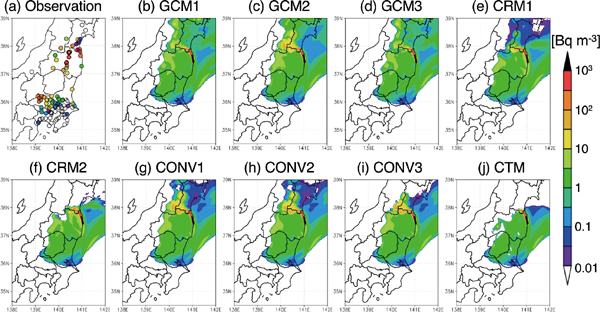
To determine differences in the simulated surface Cs-137 concentration among the experiments, representative results at specific times are shown in Fig. 3 (March 15 9:00 JST, as clusters 1 and 3), Fig. 4 (March 20 21:00 JST, as clusters 2, 3, and 6) and Fig. 5 (March 21 9:00 JST, as cluster 4). On the corresponding days, the simulated wet and dry deposition of the simulated Cs-137 is illustrated in Supplemental Figs. S1–S6. Although wet deposition can be divided into rainout and washout processes, in this model, the amount by rainout is much larger than that by washout. Thus, note that the deposit by wet deposition is almost identical to that by the rainout process in this study. On March 15 9:00 JST, Fig. 3 indicates that the observed Cs-137 concentration is the highest (10² Bq m⁻³ to 10³ Bq m⁻³) at the center of the TMA (140°E, 35.9°N), i.e., northwest Chiba and east Saitama prefectures, whereas the highest simulated Cs-137 concentrations [10 Bq m⁻³ to 10^2.5 (= 316) Bq m⁻³], except for the CRM2 and CTM experiments, occur in slightly different areas on the basis of the highest observed concentration peaks. This suggests that the simulated transport of Cs-137 in these experiments is slightly faster than that in the real world, but similar differences have often occurred in other models, mainly due to the uncertainty in the meteorological fields (e.g., Sato et al. 2018). By ignoring this difference in the position of the highest peaks, most of the experiments acceptably reproduce the observed Cs-137 concentration, except for the CRM2 and CTM experiments, which clearly yield lower simulated Cs-137 concentrations than the observed concentrations. This can be explained by the large values of the simulated wet deposition, especially around the Saitama prefecture (Fig. S1). In the GCM1, GCM2, and GCM3 experiments, the removal rate from the atmosphere through wet deposition strongly depends on the tuning parameter, GCM2 with a low f_inc value provides high Cs-137 concentrations, and a difference of approximately one order is observed at some locations. In the CRM1 experiment, the differences between the simulated and observed Cs-137 concentrations on March 15 9:00 JST (cluster 1) are small. In the CONV1, CONV2, and CONV3 experiments, the simulated Cs-137 concentrations (Fig. 3) and their dry deposition (Fig. S4) are similar to the results obtained in the CRM1 experiment, whereas the differences in the horizontal distribution of the wet deposition of the simulated Cs-137 among them are large (Fig. S1). This can be explained by relatively small amounts of wet deposition in the CONV1, CONV2, and CONV3 experiments (Fig. S1). Since the results obtained with the conventional method are theoretically similar to those obtained with the CRMtype method in the case where the autoconversion rate from cloud water into precipitation is high within the boundary layer, this suggests that autoconversion rapidly occurs on March 15 9:00 JST. As already pointed out, in the CTM experiment, the simulated Cs-137 concentrations are largely lower than those obtained in the other experiments and the observed concentrations. This suggests the overestimation of Cs-137 wet deposition. Because the CTM-type method does not always yield lower Cs-137 concentrations than the observed concentrations (e.g., Morino et al. 2013; Kajino et al. 2019), the autoconversion rate from cloud water into precipitation in the NICAM may be overestimated. In cluster 6, including the FKSM region, there are similar differences in the horizontal distribution of the simulated Cs-137 concentration among the experiments besides the differences in the peak values.

Fig. 3.

(a) Observed and (b–j) simulated Cs-137 concentrations at the surface on March 15 9:00 JST including clusters 1 and 3, as defined in Table 2. The names of the simulations correspond to the abbreviations listed in Table 1.

Fig. 4.

Same as Fig. 3 but for March 20 21:00 JST. This period includes clusters 2, 3, and 6.

Fig. 5.

Same as Fig. 3 but for March 21 9:00 JST. This period includes cluster 4.

On March 20 21:00 JST, Fig. 4 reveals that the observed Cs-137 concentration is the highest (> 10² Bq m⁻³) in FKSM, including Naka-dori (as shown in Fig. 2a) and west of Saitama in the TMA (139°E, 36°N), whereas the highest simulated Cs-137 concentrations do not occur in these areas. In Saitama, the model actually captures some peaks after the observed peak time, as shown in Fig. 6d. Although the precipitation simulation results generally agree with the JMA-estimated results (Fig. 2), differences in the simulated Cs-137 concentration among the experiments and between the NICAM and the observations occur. In Figs. S2 and S5, the wet and dry deposition of the simulated Cs-137 is not large in Naka-dori and west of Saitama. Thus, NICAM cannot reproduce the transport of the plumes. Among the experiments, the differences in the simulated Cs-137 can be explained by the same reasons, as shown in Fig. 3.

Fig. 6.

Temporal variation in the observed and simulated Cs-137 concentrations at the surface in the defined clusters listed in Table 2. Time 0 is defined as the starting time of the plumes in each cluster. The names of the simulations shown in the right panel correspond to the abbreviations listed in Table 1.

On March 21 9:00 JST, Fig. 5 shows that the observed Cs-137 concentration is the highest (> 10² Bq m⁻³) at the center of the TMA (140°E, 35.9°N), similar to the case of March 15 9:00 JST (Fig. 3). During this period, a precipitation amount of 1 mm h⁻¹ is found over several hours within a large area of the TMA (as shown in Fig. 2 in this study and Fig. 7 in Nakajima et al. 2017). Although the NICAM successfully captures this precipitation amount (as shown in Fig. 7 of Nakajima et al. 2017), the simulated precipitation in the NICAM before 24 hours is higher than the observed precipitation (Fig. 2). Consequently, all of the experiments yield lower simulated Cs-137 concentrations than the observed Cs-137 concentrations. Apparently, the wet deposition of the simulated Cs-137, especially in the CRM2 and CTM experiments, over the FKSM region is larger than that in the other experiments (Fig. S3), whereas the dry deposition of the simulated Cs-137 in the CRM2 and CTM experiments over the FKSM region is slightly smaller than that in the other experiments (Fig. S6).

Fig. 7.

Statistical metrics defined in Appendix based on the simulated and observed Cs-137 concentrations at the 100 available sites. The metrics include the (a) geometric mean bias (GMB), (b) normalized mean bias (NMB), (c) Pearson correlation coefficient (PCC), (d) root-mean-square-error (RMSE), (e) fraction of data within a factor of 2 to the observations (FA2), and (f) fraction of data within a factor of 10 (FA10) to the observations.

In summary, as shown in Figs. 3 and 4, underestimation of the simulated Cs-137 concentration in the CTM experiments is caused by an overestimation of the wet deposition flux (Figs. S1–S3), which depends on the spatiotemporal distributions of clouds and precipitation in the atmosphere. This indicates that the conversion rate from cloud water into precipitation in the NICAM is high, which is a common problem, as previously pointed out in other studies (Suzuki et al. 2015; Jing and Suzuki 2018). The uncertainty in the simulated Cs-137 concentration with the GCM-type method considering various scavenging coefficient values (f_inc ranges from 0.01 to 0.9, which is within the range of the tuning factor) is comparable to the difference between the GCM- and CRM-type methods. Although no precipitation is observed in the TMA area on March 21 9:00 JST, there are small differences in the simulated Cs-137 concentration among the different tuning parameters under the GCM-type method. This indicates that the GCM-type method does not strongly depend on the surface precipitation flux. Among the results of the CONV1, CONV2, and CONV3 experiments, the difference in the simulated Cs-137 concentration on March 21 9:00 JST (Fig. 5) is larger than that on March 15 9:00 JST (Fig. 3) and March 20 21:00 JST (Fig. 4). Particularly, the simulated Cs-137 concentrations in the CONV1 and CONV2 experiments are closer to the observation and higher than those in the CONV3 experiments due to the high wet deposition in the CONV3 experiment, which sets too large values of B in Eq. (6).

3.3 Temporal distribution of the Cs-137 concentration

To examine the reproducibility of the simulated plumes (including Cs-137 concentrations higher than 10 Bq m⁻³), the temporal variations in each cluster are shown in Fig. 6. In cluster 2, as shown in Figs. 4, 6b, and 6f, most of the simulated Cs-137 concentrations over the Tohoku area (only Miyagi and Yamagata prefectures) generally agree with the observed results. In FKSM (cluster 6), as shown in Fig. 6f, the differences in the simulated Cs-137 concentration among the experiments are small, and the wet deposition scheme is less important in this case, i.e., transport is more important. Figure 6b shows the coincidence of the start times of the observed and simulated peaks with a high variability in the end times of the peaks. At the end of a peak, the simulated Cs-137 concentrations are generally lower than the observed concentrations, except for CRM1, CONV1, CONV2, and CONV3. In the CRM2 and CTM experiments, the simulated Cs-137 concentrations at 3 h before the peak are also underestimated.

In cluster 1, as shown in Figs. 3 and 6a, a high variability occurs in the simulated Cs-137 concentration among the experiments, but none of the experiments succeeds in reproducing the temporal variation in the observed Cs-137 concentration. Before the start of a peak, the simulated Cs-137 concentrations are overestimated, whereas after a peak, the simulated Cs-137 concentrations are lower than the observed concentrations. This indicates that none of the models reproduces the high observed concentrations over more than 3 h. Figure 6a clearly shows the difference in the simulated Cs-137 concentration among the experiments, which supports the two findings described in Section 3.2. First, the GCM-type method (i.e., GCM2) generally provides comparable results to those provided by the CRM-type method (i.e., CRM1). Second, the conventional method (i.e., CONV2) effectively reproduces the observations and generally yields much better results than those yielded by many physical-based methods (the GCM- and CTM-type methods). This implies that the complex nature of simulating hydrometeors is close to the observation compared to approximating the surface precipitation rate. Figures 6d and 6e show that the peak timings are off by approximately 3 h or 4 h between the observation and simulations, and the magnitudes tend to be underestimated. Finally, Fig. 6c shows the entire underestimation range of the simulated Cs-137 concentration, as shown in Fig. 5. This should be addressed via improvement of the transport patterns through modification of the meteorological fields nudged in the NICAM simulation.

With the use of the hourly datasets at all available sites, statistical metrics such as bias, uncertainty, and precision are compared among the experiments (Fig. 7). The definition of each factor is explained in Appendix, and these metrics have often been adopted in other studies (Kitayama et al. 2018; Sato et al. 2018). In this study, the total sampling number was 6837 for all 100 sites. The geometric mean bias (GMB) values were within ±15 % (GCM2, CRM1, CONV2, and CONV3) and ±30 % (GCM1, GCM3, and CRM2), whereas outliers occurred (1.39 in CONV1 and 0.44 in CTM). The results of the experiments with a high GMB tend to provide high normalized mean bias (NMB) values at −55.9 % (CTM) and +38.6 % (CONV1). Except for these values, the calculated NMB was within ±15 % (GCM2, CRM1, and CONV3) and ±30 % (the remaining experiments). The correlation was determined with the Pearson correlation coefficient (PCC). The calculated PCC values in all experiments ranged from 0.60 (CONV1) to 0.89 (CTM) (which indicates that the models generally exhibit a moderate-to-high correlation). The uncertainty is expressed as the root-mean-square error (RMSE). High negative GMB and NMB values (CTM) yield small RMSE values (53.5 Bq m⁻³), whereas low GMB and NMB values produce RMSE values ranging from 66.9 Bq m⁻³ to 111.6 Bq m⁻³. The precision is expressed as the fraction of the observations reproduced by the simulations within a factor of 2 (FA2) or 10 (FA10). In this study, the values of both FA2 and FA10 were low, at < 13 % for FA2 and < 41 % for FA10. The FA10 values obtained in the GCM2, CRM1, CONV1, and CONV2 experiments exceeded 30 % and were higher than those obtained in the other experiments. Overall, GCM2, CRM1, and CONV2 yielded better results.

3.4 Total amount of deposition in March 2011

Figure 8 shows the wet and dry deposition amounts and the fraction of the total deposition over land to that over all areas in March 2011. The horizontal distributions are shown in Fig. 9. The observed amount of Cs-137 deposited over land is 2.50 PBq, whereas the simulated amount ranges from 0.59 PBq (CONV1) to 3.16 PBq (GCM3). In Section 3.3, the experiments (GCM2, CRM1, and CONV2) showed better results of the surface Cs-137 concentrations in the value of 2.01 PBq (GCM2), 1.57 PBq (CRM1), and 1.62 PBq (CONV2), which are lower than the observed amount by 20–37 %. For example, GCM2 has an NMB of −2.7 % for Cs-137 concentrations and a bias of −20 % for Cs-137 total deposition over land. In contrast, the results in the experiments (CRM2 and CTM) showed a larger negative bias for the surface Cs-137 concentrations in Section 3.3, likely high fluxes of wet deposition. The resulting value of 1.7 PBq is also lower than the observed amount by 30 %. These seemingly inconsistent relationships are also found in the previous studies (e.g., Kitayama et al. 2018; Sato et al. 2018). This may be caused by the uncertainty of the emission source term (Katata et al. 2015) used in this study and these MIPs. In most of the experiments, wet deposition, which is mainly rainout in this study with a range from 1.35 PBq to 2.98 PBq, is larger than the dry deposition with a range from 0.10 PBq to 0.27 PBq, except for the CONV1 experiment. The fraction of the wet deposition to total deposition over land ranged from 83 % to 94 % in most experiments, except for the CONV1 experiment. The CONV1 experiment has 0.27 PBq of the wet deposition, 0.32 PBq of the dry deposition, and 45 % of the fraction of the wet deposition to the total deposition over land. The possible reason is that the low value of B in Eq. (6) in the CONV1 experiment (B = 0.08) forces less wet deposition and more dry deposition.

Fig. 8.

(a) Total deposition amount, i.e., wet and dry deposition amount, over land in the experiments and flight observations (in units of PBq) and (b) fraction of the total deposition amount over land to that over all areas (in units of %). The observation in panel (a) cannot be divided into wet and dry deposition.

Fig. 9.

Horizontal distribution of the observed and simulated Cs-137 deposition amounts in March 2011 (in units of kBq m⁻²).

The fractions of the total deposition over land to that over all areas range from 21.2 % (CTM) to 44.4 % (GCM3), which can be separated into two groups depending on the wet deposition amount. Most of the results range from 35 % to 44 %, which is comparable to the average value among MIPs (Sato et al. 2018). The CRM2, CONV1, and CTM experiments yield low fractions over land with values ranging from 21 % to 25 %. This indicates that these experiments (CRM2 and CTM) consider a large deposition amount of Cs-137 over the ocean, especially near the FDNPP (Fig. 9), whereas the CONV1 experiment has a low deposition amount of Cs-137 over all areas (Fig. 8a). In the FKSM prefecture, the observed fluxes of Cs-137 from the FDNPP to central FKSM (Naka-dori) are hardly reproduced by the NICAM and the other models, as reported in Sato et al. (2018), probably due to Cs-137 transport issues along complex terrain in the FKSM. In Tochigi and Gunma, underestimation occurs in all experiments, whereas in Ibaraki, slight overestimation occurs in the GCM1, GCM2, GCM3, and CTM experiments, comparable results occur in the CRM1 experiment, and the underestimation occurs in the CRM2, CONV1, CONV2, and CONV3 experiments. In northern Miyagi, the observed deposition ranges more than 10 kBq m⁻² mainly due to the wet deposition on March 22 as suggested by Sanada et al. (2018), but all experiments overly underestimate.

The above validation of the simulated Cs-137 distribution leads to the following conclusions. Regarding the validation of the surface Cs-137 concentration shown in Sections 3.2 and 3.3, the results of the GCM2, CRM1, and CONV2 experiments are closer to the observed concentrations when compared with the other experiments with a mean bias of less than 20 %. As shown in this section, the deposition results of these better experiments in the surface Cs-137 concentration, i.e., GCM2, CRM1, and CONV2, are approximately 20–40 % lower than the observations. These underestimations of both the surface concentration and deposit of the simulated Cs-137 may be explained by the uncertainty of the source term (Katata et al. 2015) and the meteorological fields (Sekiyama et al. 2015). When the differences in the results among the experiments are focused, it is difficult to conclude the best method of the rainout process in this study, but it can be concluded that the GCM-type and conventional methods suitably reproduce the results obtained with the CRM-type method by tuning a parameter. However, the CRM-type method contains a more physical formulation than the GCM-type method because the newly formed hydrometeors flux used in Eq. (5) in the CRM-type is explicitly prognosed. Although the tuning parameters of f_inc are set to very low values (0.1 in the GCM2 experiment and 0.01 in the CRM1), which may not be accepted even within the uncertainty of f_inc, this implies another problem of our model, NICAM. That is, the overestimation of the conversion rate from cloud water to precipitation in the NICAM causes the overestimation of the wet deposition amount. To compensate for this, the f_inc should be set to low in the GCM 2 and CRM1 experiments. Note that when the high conversion rate from cloud water into precipitation in the NICAM is correctly fixed, the CTM-type may have much better results since the CTM-type has high correlation and low uncertainty.

3.5 Sensitivity of the simulated Cs-137 concentration to the cloud microphysics treatments

Cloud microphysics treatments affect the simulated Cs-137 concentration via modulation of the aerosol–cloud–precipitation interaction. To investigate their impacts, a different cloud microphysics model, NDW6, developed by Seiki and Nakajima (2014), is adopted in the NICAM. According to previous studies, such as Sato et al. (2015), NDW6 tends to provide lower precipitation than NSW6. In this study, it was found that the difference in the simulated precipitation between NSW6 and NDW6 was small, and the results obtained with NDW6 were still higher than the observations. The additional sensitivity experiments considering a different autoconversion process, KK00, also provided similar precipitation amounts to the results provided by the original autoconversion process of BE68. Figure 10 shows the simulated Cs-137 concentration at the clustered sites, as shown in Fig. 6. The impacts of the various autoconversion processes on the differences between the simulated Cs-137 concentrations are not zero but small at all clusters in both the CRM1 and CTM experiments. In cluster 2, for example, the Cs-137 concentration simulated by the CTM with NDW6 is closer to the observed concentrations than that simulated by the CTM with NSW6. Nevertheless, the differences among the various cloud microphysics treatments are smaller than those among the various tuning results (CRM2) and wet deposition modules, as shown in Fig. 6. Figure 11 shows the variability in the statistical metrics calculated based on the simulated and observed Cs-137 concentrations at the surface, as already shown in Fig. 7. This figure clearly shows that the variability among the different cloud microphysics treatments is lower than that among the different wet deposition modules and tuning parameters in wet deposition. One possibility explaining these results is that cloud fields, especially those related to aerosol wet deposition, are dominated not by aerosol–cloud microphysics but by synoptic-scale meteorological conditions. Another explanation is that the nudging of the meteorological fields, i.e., wind, temperature, and water vapor, weakens the variability in clouds and precipitation. These findings suggest that the differences in the cloud microphysics treatments among the various models, similar to MIPs, do not primarily cause the differences in the simulated Cs-137 distribution. Thus, to truly improve the reproducibility of Cs-137 aerosol simulations, basic meteorological fields such as wind and water vapor, which basically reproduce model cloud macrophysics, should be enhanced.

Fig. 10.

Same as Fig. 6 but regarding the additional sensitivity experiments related to the cloud microphysics treatments. The names of the experiments are listed in the right panel, which includes the observations, the original sensitivity experiments (CRM1, CRM2, and CTM, as listed in Table 1), and the extra sensitivity experiments considering several treatments, including autoconversion from clouds into precipitation, KK00, and the two-moment bulk cloud microphysics model, NDW6.

Fig. 11.

Uncertainties, i.e., variabilities among the categorized experiments, in the statistical metrics [(a) mean value, (b) GMB, (c) PCC, (d) NMB, (e) RMSE (f) FA2, and (g) FA10], as defined in Appendix and shown in Fig. 7. The categorized experiments are d-schemes (different wet deposition modules), d-finc (different f_inc parameter values in CRM1 and CRM2), and d-clouds (the additional sensitivity experiments based on CRM1 regarding the cloud microphysics treatments).

4. Conclusions

We newly categorized the observed Cs-137 plumes emitted by the FDNPP into six groups, depending on the region and period (Table 2). The 418 (55 sites) samples with observed concentrations > 10 Bq m⁻³ are considered, including 234 samples obtained at 15 sites in FKSM (located near the FDNPP) and 184 samples obtained at 40 sites in the other prefectures. With these 418 samples, we distinguished six clusters according to the following rules: (1) The start time is set to 3 h before a peak occurs at any site in the same cluster. (2) The end time is set to 3 h after the last peak at any site in the same cluster. Out of the six clusters, three are located in the TMA, two occur in FKSM and the remaining is located in the Tohoku region (northern part of Japan Island).

Although relatively simple GCM-type and conventional schemes of rainout process, which is the main deposition for the particulate Cs-137 in the fine mode, respond well to the tuning parameter and attains the good approximation of the aerosol simulations close to the observation, the CRM-type method can provide some of the best results on the Cs-137 concentration, although it is highly sensitive to the physics of the model. The CTM-type method generally underestimates the Cs-137 concentration due to the overestimation of the wet deposition flux, which depends on the cloud and precipitation distributions in the atmosphere (not only the surface). This indicates that the high conversion rate from cloud water into precipitation in the NICAM is common among GCMs and CRMs (Suzuki et al. 2015; Jing and Suzuki 2018).

In most experiments, the statistical metrics using the surface Cs-137 concentrations are calculated to be within ±30 % (normalized bias: NMB), 0.6–0.9 (correlation: PCC), 67–112 Bq m⁻³ (uncertainty: RMSE), and < 40 % (precision: FA10). The simulated total deposition amounts over land are generally underestimated by 20–40 % (most of the models: 1.6–2.1 PBq; observation: 2.5 PBq). In most of the experiments, the fraction of the wet deposition to total deposition over land ranged from 83 % to 94 % in most experiments. Since the deposition amounts of rainout are much larger than those of washout, it can be concluded that the effect of the rainout process on the overall removal process is overwhelmingly greater than that of other processes. The fractions of the total deposition amount over land to that over all areas range from 21 % to 44 %, with the variation relating to the total deposition amount. Most of the results are approximately 40 %, which is comparable with the average amount across MIPs (Sato et al. 2018).

Regarding the surface Cs-137 concentration shown in Sections 3.2 and 3.3, the results of the GCM2, CRM1, and CONV2 experiments are closer to the observed concentrations compared to the other experiments with a mean bias of less than 20 %. In Section 3.4, the results of these experiments, i.e., GCM2, CRM1, and CONV2, exhibit a 20–40 % underestimation of the deposition over land. These underestimations of both the surface concentration and deposit of the simulated Cs-137 may be explained by the uncertainty of the source term (Katata et al. 2015) and the meteorological fields (Sekiyama et al. 2015). In terms of the wet deposition process among the sensitivity experiments, it is difficult to determine the best method of the rainout process in this study, but it can be concluded that the CRM-type method contains a more physical formulation than the GCM-type and conventional methods because the newly formed hydrometeors flux used in Eq. (5) in the CRM-type is explicitly prognosed. Thus, the CRM1 experiment may be adopted as a new formal version, although the tuning parameter of f_inc is set to very low, which may not be apart from reality. This also implies the overestimation of the conversion rate from cloud water to precipitation in the NICAM, which causes the overestimation of the wet deposition amount. To compensate for it, the f_inc should be set to low. It should also be noted that both the GCM-type method with proper tuning parameters and the conventional method remain useful. The CTM-type may have much better results when the high conversion rate from cloud water into precipitation in the NICAM is correctly fixed since the CTM-type has a high correlation and low uncertainty.

Since a high conversion rate from cloud water into precipitation in the NICAM is suggested in this study, sensitivity experiments of various cloud microphysics treatments to the simulated Cs-137 concentration are performed. These extra experiments are conducted with different cloud microphysics treatments: (1) change in the cloud microphysics scheme from NSW6 to NDW6 and (2) change in the autoconversion scheme from BE68 to KK00. The impacts on the simulated Cs-137 concentration are smaller than those of the different wet deposition schemes. One possibility is that cloud fields, especially those related to aerosol wet deposition, are dominated not by aerosol–cloud microphysics but by synoptic-scale meteorological conditions. Another possibility is that the nudging of meteorological fields, i.e., wind, temperature, and water vapor, weakens the variability in clouds and precipitation. These findings suggest that the differences in cloud microphysics treatments among the various models, e.g., MIPs, do not primarily cause the differences in the simulated Cs-137 distribution. Saya et al. (2018) suggested that a better simulation of precipitation provides a closer deposition amount of simulated Cs-137 to the observation. Sekiyama et al. (2021) implied that the high accuracy of the simulated Cs-137 needs much higher accuracy of the meteorological fields. To improve the reproducibility of Cs-137 aerosol simulations, it is important to have an accurate set of basic meteorological fields, i.e., wind and water vapor, which determine the transport and deposition of Cs-137 as well as proper rainout parameterizations and tunings.

Data Availability Statement

The model results used to support this article can be obtained from the corresponding author upon request ([e-mail]). The observational data of Cs-137 are freely accessible in Appendix A of Oura et al. (2015) at http://www.radiochem.org/paper/JN152/jn15201_Appendix_A_rev.pdf (last access: March 1, 2021).

Supplements

Supplemental Figs. S1–S6 shows the horizontal distribution of the 24-hour accumulated deposition amount of the simulated Cs-137 by wet and dry deposition on specific times (March 14 9:00 JST to 15 9:00 JST, March 19 21:00 JST to 20 9:00 JST, and March 20 9:00 JST to 21 9:00 JST).

Acknowledgments

We thank the developers and administrators of the NICAM (http://nicam.jp/; last access: March 1, 2021) and the principal investigators of the monitoring sites considered in this study. The horizontal maps in the figures are drawn with Grid Analysis and Display System (GrADS) software (http://cola.gmu.edu/grads, last access: March 1, 2021). The model simulations and analysis were mainly performed with the supercomputer of the University of Tokyo/Oakforest-PACS and supplementally used with the following supercomputers: NIES/NEC SX-Aurora TSUBASA, JAXA/JSS2, and JAXA/JSS3. This research was supported by the following grants: the Environment Research and Technology Development Fund of the Environmental Restoration and Conservation Agency, Japan (S-12: JPMEERF14S11200, 1-1802: JPMEERF2018 1002, 1-1501: JPMEERF20155001, and S-20-1(3): JPMEERF21S12003), JSPS KAKENHI (17H04711 and 19H05669), and JAXA/GCOM-C. We acknowledge Yu Morino for discussing the model framework of CMAQ.

Appendix: Definition of metrics

To evaluate the statistical results, the following metrics are introduced (e.g., Chang and Hanna 2004; Goto et al. 2020a):

A.1 Geometric mean bias (GMB) in Eq. (A1)

  

A.2 Normalized mean bias (NMB) in Eq. (A2)

  

A.3 Root-mean-square error (RMSE) in Eqs. (A3a) and (A3b)

  

  

A.4 Pearson correlation coefficient (PCC) in Eq. (A4)

  

A.5 Fraction of the data within a factor of two to the observations (FA2) in Eq. (A5)

FA2 = fraction of data that satisfy;   

A.6 Fraction of the data within a factor of ten to the observations (FA10) in Eq. (A6)

FA10 = fraction of data that satisfy;   

Statistical calculations are performed with the hourly datasets obtained at 100 available sites, which range from 0.01 (set to the minimum value in the observations as the detection limit) to 10⁵ Bq m⁻³, and in the case where the observed Cs-137 concentration exceeds the detection limit.

Data Availability Statement

The model results used to support this article can be obtained from the corresponding author upon request ([e-mail]). The observational data of Cs-137 are freely accessible in Appendix A of Oura et al. (2015) at http://www.radiochem.org/paper/JN152/jn15201_Appendix_A_rev.pdf (last access: March 1, 2021).

References

•  Balkanski,  Y. J.,  D. J.  Jacob,  G. M  Gardner,  W. C.  Gaustein, and  K. K.  Turekian, 1993: Transport and residence times of tropospheric aerosols inferred from a global three-dimensional simulation of ²¹⁰Pb. J. Geophys. Res., 98, 20573-20586.
•  Berry,  E. X., 1968: Modification of the Warm Rain Process. Proceedings of the first conference on weather modification, Albany, NY, 81-85.
•  Binkowski,  F. S., and  S. J.  Roselle, 2003: Models-3 Community Multiscale Air Quality (CMAQ) model aerosol component. 1. Model description. J. Geophys. Res., 108, 4183, doi:10.1029/2001JD001409.
•  Byun,  D., and  K. L.  Schere, 2006: Review of the governing equations, computational algorithms, and other components of the Model-3 Community Multiscale Air Quality (CMAQ) modeling system. Appl. Mech. Rev., 59, 51-77.
•  Chang,  J. C., and  S. R.  Hanna, 2004: Air quality model performance evaluation. Meteor. Atmos. Phys., 87, 167-196.
•  Chen,  L.,  Y.  Gao,  M.  Zhang,  J. S.  Fu,  J.  Zhu,  H.  Liao,  J.  Li,  K.  Huang,  B.  Ge,  X.  Wang,  Y. F.  Lam,  C.-Y.  Lin,  S.  Itahashi,  T.  Nagashima,  M.  Kajino,  K.  Yamaji,  Z.  Wang, and  J.  Kurokawa, 2019: MICS-Asia III: Multimodel comparison and evaluation of aerosol over East Asia. Atmos. Chem. Phys., 19, 11911-11937.
•  Giorgi,  F., and  W. L.  Chameides, 1986: Rainout lifetimes of highly soluble aerosols and gases as inferred from simulations with a general circulation model. J. Geophys. Res., 91, 14367-14376.
•  Goto,  D.,  T.  Dai,  M.  Satoh,  H.  Tomita,  J.  Uchida,  S.  Misawa,  T.  Inoue,  H.  Tsuruta,  K.  Ueda,  C. F. S.  Ng,  A.  Takami,  N.  Sugimoto,  A.  Shimizu,  T.  Ohara, and  T.  Nakajima, 2015: Application of a global nonhydrostatic model with a stretched-grid system to regional aerosol simulations around Japan. Geosci. Model Dev., 8, 235-259.
•  Goto,  D.,  K.  Ueda,  C. F. S.  Ng,  A.  Takami,  T.  Ariga,  K.  Matsuhashi, and  T.  Nakajima, 2016: Estimation of excess mortality due to long-term exposure to PM2.5 in Japan using a high-resolution model for present and future scenarios. Atmos. Environ., 140, 320-332.
•  Goto,  D.,  M.  Kikuchi,  K.  Suzuki,  M.  Hayasaki,  M.  Yoshida,  T. M.  Nagao,  M.  Choi,  J.  Kim,  N.  Sugimoto,  A.  Shimizu,  E.  Oikawa, and  T.  Nakajima, 2019: Aerosol model evaluation using two geostationary satellites over East Asia in May 2016. Atmos. Res., 217, 93-113.
•  Goto,  D.,  Y.  Morino,  T.  Ohara,  T. T.  Sekiyama,  J.  Uchida, and  T.  Nakajima, 2020a: Application of linear minimum variance estimation to the multi-model ensemble of atmospheric radioactive Cs-137 with observations. Atmos. Chem. Phys., 20, 3589-3607.
•  Goto,  D.,  Y.  Sato,  H.  Yashiro,  K.  Suzuki,  E.  Oikawa,  R.  Kudo,  T. M.  Nagao, and  T.  Nakajima, 2020b: Global aerosol simulations using NICAM.16 on a 14 km grid spacing for a climate study: Improved and remaining issues relative to a lower-resolution model. Geosci. Model Dev., 13, 3731-3768.
•  Han,  Z.,  T.  Sakurai,  H.  Ueda,  G. R.  Carmichael,  D.  Streets,  H.  Hayami,  Z.  Wang,  T.  Holloway,  M.  Engardt,  Y.  Hozumi,  S. U.  Park,  M.  Kajino,  K.  Sartelet,  C.  Fung,  C.  Bennet,  N.  Thongboonchoo,  Y.  Tang,  A.  Chang,  K.  Matsuda, and  M.  Amann, 2008: MICS-Asia II: Model intercomparison and evaluation of ozone and relevant species. Atmos. Environ., 42, 3491-3509.
•  Henzing,  J. S.,  D. J. L.  Olivié, and  P. F. J.  van Velthoven, 2006: A parameterization of size resolved below cloud scavenging of aerosols by rain. Atmos. Chem. Phys., 6, 3363-3375.
•  Jing,  X., and  K.  Suzuki, 2018: The impact of process-based warm rain constraints on the aerosol indirect effect. Geophys. Res. Lett., 45, 10729-10737.
•  Kajino,  M.,  T. T.  Sekiyama,  A.  Mathieu,  I.  Korsakissok,  R.  Périllat,  D.  Quélo,  A.  Quérel,  O.  Saunier,  K.  Adachi,  S.  Girard,  T.  Maki,  K.  Yumimoto,  D.  Didier,  O.  Masson, and  Y.  Igarashi, 2018: Lessons learned from atmospheric modeling studies after the Fukushima nuclear accident: Ensemble simulations, data assimilation, elemental process modeling, and inverse modeling. Geochem. J., 52, 85-101.
•  Kajino,  M.,  T. T.  Sekiyama,  Y.  Igarashi,  G.  Katata,  M.  Sawada,  K.  Adachi,  Y.  Zaizen,  H.  Tsuruta, and  T.  Nakajima, 2019: Deposition and dispersion of radio-Cesium released due to the Fukushima nuclear accident: Sensitivity to meteorological models and physical modules. J. Geophy. Res.: Atmos., 124, 1823-1845.
•  Kaneyasu,  N.,  H.  Ohashi,  F.  Suzuki,  T.  Okuda, and  F.  Ikemori, 2012: Sulfate aerosol as a potential transport medium of radiocesium from the Fukushima nuclear accident. Environ. Sci. Technol., 46, 5720-5726.
•  Katata,  G.,  M.  Chino,  T.  Kobayashi,  H.  Terada,  M.  Ota,  H.  Nagai,  M.  Kajino,  R.  Draxler,  M. C.  Hort,  A.  Malo,  T.  Torii, and  Y.  Sanada, 2015: Detailed source term estimation of the atmospheric release for the Fukushima Daiichi Nuclear Power Station accident by coupling simulations of an atmospheric dispersion model with an improved deposition scheme and oceanic dispersion model. Atmos. Chem. Phys., 15, 1029-1070.
•  Khairoutdinov,  M., and  Y.  Kogan, 2000: A new cloud physics parameterization in a large-eddy simulation model of marine stratocumulus. Mon. Wea. Rev., 128, 229-243.
•  Kitayama,  K.,  Y.  Morino,  M.  Takigawa,  T.  Nakajima,  H.  Hayami,  H.  Nagai,  H.  Terada,  K.  Saito,  T.  Shimbori,  M.  Kajino,  T. T.  Sekiyama,  D.  Didier,  A.  Mathieu,  D.  Quélo,  T.  Ohara,  H.  Tsuruta,  Y.  Oura,  M.  Ebihara,  Y.  Moriguchi, and  T.  Shibata, 2018: Atmospheric modeling of 137Cs plumes from the Fukushima Daiichi Nuclear Power Plant—Evaluation of the model intercomparison data of the science council of Japan. J. Geophy. Res.: Atmos., 123, 7754-7770.
•  Leadbetter,  S. J.,  M. C.  Hort,  A. R.  Jones,  H. N.  Webster, and  R. R.  Draxler, 2015: Sensitivity of the modelled deposition of Caesium-137 from the Fukushima Daiichi nuclear power plant to the wet deposition parameterization in NAME. J. Environ. Radioact., 139, 200-211.
•  Liu,  H.,  D. J.  Jacob,  I.  Bey, and  R. M.  Yantosca, 2001: Constraints from ²¹⁰Pb and ⁷Be on wet deposition and transport in a global three-dimensional chemical tracer model driven by assimilated meteorological fields. J. Geophys. Res., 106, 12109-12128.
•  Michibata,  T., and  T.  Takemura, 2015: Evaluation of autoconversion schemes in a single model framework with satellite observation. J. Geophys. Res.: Atmos., 120, 9570-9590.
•  Morino,  Y.,  T.  Ohara,  M.  Watanabe,  S.  Hayashi, and  M.  Nishizawa, 2013: Episode analysis of deposition of radiocesium from the Fukushima Daiichi nuclear power plant accident. Environ. Sci. Technol., 47, 2314-2322.
•  Myhre,  G.,  B. H.  Samset,  M.  Schulz,  Y.  Balkanski,  S.  Bauer,  T. K.  Berntsen,  H.  Bian,  N.  Bellouin,  M.  Chin,  T.  Diehl,  R. C.  Easter,  J.  Feichter,  S. J.  Ghan,  D.  Hauglustaine,  T.  Iversen,  S.  Kinne,  A.  Kirkevåg,  J.-F.  Lamarque,  G.  Lin,  X.  Liu,  M. T.  Lund,  G.  Luo,  X.  Ma,  T.  van Noije,  J. E.  Penner,  P. J.  Rasch,  A.  Ruiz,  Ø.  Seland,  R. B.  Skeie,  P.  Stier,  T.  Takemura,  K.  Tsigaridis,  P.  Wang,  Z.  Wang,  L.  Xu,  H.  Yu,  F.  Yu,  J.-H.  Yoon,  K.  Zhang,  H.  Zhang, and  C.  Zhou, 2013: Radiative forcing of the direct aerosol effect from AeroCom Phase II simulations. Atmos. Chem. Phys., 13, 1853-1877.
•  Nagata,  K., 2011: Quantitative precipitation estimation and quantitative precipitation forecasting by the Japan Meteorological Agency. Japan Meteorol. Agency-Technical Rev., 13, 37-50.
•  Nakajima,  T.,  S.  Misawa,  Y.  Morino,  H.  Tsuruta,  D.  Goto,  J.  Uchida,  T.  Takemura,  T.  Ohara,  Y.  Oura,  M.  Ebihara, and  M.  Satoh, 2017: Model depiction of the atmospheric flows of radioactive cesium emitted from the Fukushima Daiichi Nuclear Power Station accident. Prog. Earth Planet. Sci., 4, 2, doi:10.1186/s40645-017-0117-x.
• Nuclear Regulation Authority, 2012: Airborne monitoring results in each prefecture. Nuclear Regulation Authority. [Available at: https://radioactivity.nsr.go.jp/en/list/203/list-1.html.]
•  Oura,  Y.,  M.  Ebihara,  H.  Tsuruta,  T.  Nakajima,  T.  Ohara,  M.  Ishimoto,  H.  Sawahata,  Y.  Katsumura, and  W.  Nitta, 2015: A database of hourly atmospheric concentrations of radiocesium (¹³⁴Cs and ¹³⁷Cs) in suspended particulate matter collected in March 2011 at 99 air pollution monitoring stations in eastern Japan. J. Nucl. Radiochem. Sci., 15, 2_1-2_12.
•  Quérel,  A.,  Y.  Roustan,  D.  Quélo, and  J.-P.  Benoit, 2015: Hints to discriminate the choice of wet deposition models applied to an accidental radioactive release. Int. J. Environ. Pollut., 58, 268-279.
•  Sanada,  Y.,  G.  Katata,  N.  Kaneyasu,  C.  Nakanishi,  Y.  Urabe, and  Y.  Nishizawa, 2018: Altitudinal characteristics of atmospheric deposition of aerosols in mountainous regions: Lessons from the Fukushima Daiichi Nuclear Power Station accident. Sci. Total Environ., 618, 881-890.
•  Sato,  Y.,  S.  Nishizawa,  H.  Yashiro,  Y.  Miyamoto,  Y.  Kajikawa, and  H.  Tomita, 2015: Impacts of cloud microphysics on trade wind cumulus: Which cloud microphysics processes contribute to the diversity in a large eddy simulation? Prog. Earth Planet. Sci., 2, 23, doi:10.1186/s40645-015-0053-6.
•  Sato,  Y.,  M.  Takigawa,  T. T.  Sekiyama,  M.  Kajino,  H.  Terada,  H.  Nagai,  H.  Kondo,  J.  Uchida,  D.  Goto,  D.  Quélo,  A.  Mathieu,  A.  Quérel,  S.  Fang,  Y.  Morino,  P.  von Schoenberg,  H.  Grahn,  N.  Brännström,  S.  Hirao,  H.  Tsuruta,  H.  Yamazawa, and  T.  Nakajima, 2018: Model intercomparison of atmospheric ¹³⁷Cs from the Fukushima Daiichi Nuclear Power Plant accident: Simulations based on identical input data. J. Geophys. Res.: Atmos., 123, 11748-11765.
•  Sato,  Y.,  T. T.  Sekiyama,  S.  Fang,  M.,  Kajino,  A.  Quérel,  D.  Quélo,  H.  Kondo,  H.  Terada,  M.  Kadowaki,  M.  Takigawa,  Y.  Morino,  J.  Uchida,  D.  Goto, and  H.  Yamazawa, 2020: A model intercomparison of atmospheric ¹³⁷Cs concentrations from the Fukushima Daiichi Nuclear Power Plant accident, Phase III: Simulation with an identical source term and meteorological field at 1-km resolution. Atmos. Environ., X7, 100086, doi:10.1016/j.aeaoa.2020.100086.
•  Satoh,  M.,  H.  Tomita,  H.  Yashiro,  H.  Miura,  C.  Kodama,  T.  Seiki,  A. T.  Noda,  Y.  Yamada,  D.  Goto,  M.  Sawada,  T.  Miyoshi,  Y.  Niwa,  M.  Hara,  T.  Ohno,  S.  Iga,  T.  Arakawa,  T.  Inoue, and  H.  Kubokawa, 2014: The Nonhydrostatic icosahedral atmospheric model: Description and development. Prog. Earth Planet. Sci., 1, 18, doi:10.1186/s40645-014-0018-1.
•  Saya,  A.,  T.  Yoshikane,  E.-C.  Chang,  K.  Yoshimura, and  T.  Oki, 2018: Precipitation redistribution method of regional simulations of radioactive material transport during the Fukushima Daiichi Nuclear Power Plant accident. J. Geophy. Res.: Atmos., 123, 10248-10259.
•  Schulz,  M.,  C.  Textor,  S.  Kinne,  Y.  Balkanski,  S.  Bauer,  T.  Berntsen,  T.  Berglen,  O.  Boucher,  F.  Dentener,  S.  Guibert,  I. S. A.  Isaksen,  T.  Iversen,  D.  Koch,  A.  Kirkevåg,  X.  Liu,  V.  Montanaro,  G.  Myhre,  J. E.  Penner,  G.  Pitari,  S.  Reddy,  Ø.  Seland,  P.  Stier, and  T.  Takemura, 2006: Radiative forcing by aerosols as derived from the AeroCom present-day and pre-industrial simulations. Atmos. Chem, Phys., 6, 5225-5246.
•  Seiki,  T., and  T.  Nakajima, 2014: Aerosol effects of the condensation process on a convective cloud simulation. J. Atmos. Sci., 71, 833-853.
•  Seiki,  T.,  C.  Kodama,  A. T.  Noda, and  M.  Satoh, 2015: Improvement in global cloud-system-resolving simulations by using a double-moment bulk cloud microphysics scheme. J. Climate, 28, 2405-2419.
•  Sekiyama,  T. T.,  M.  Kunii,  M.  Kajino, and  T.  Shimbori, 2015: Horizontal resolution dependence of atmospheric simulations of the Fukushima nuclear accident using 15-km, 3-km, and 500-m grid models. J. Meteor. Soc. Japan, 93, 49-64.
•  Sekiyama,  T. T.,  M.  Kajino, and  M.  Kunii, 2021: Ensemble dispersion simulation of a point-source radioactive aerosol using perturbed meteorological fields over Eastern Japan. Atmosphere, 12, 662, doi:10.3390/atmos12060662.
•  Seinfeld,  J. H., and  S. N.  Pandis, 2006: Atmospheric Chemistry and Physics: From Air Pollution to Climate Change. John Wiley and Sons, 1203 pp.
•  Shindell,  D. T.,  M.  Chin,  F.  Dentener,  R. M.  Doherty,  G.  Faluvegi,  A. M.  Fiore,  P.  Hess,  D. M.  Koch,  I. A.  MacKenzie,  M. G.  Sanderson,  M. G.,  Schultz,  M.  Schulz,  D. S.  Stevenson,  H.  Teich,  C.  Textor,  O.  Wild,  D. J.  Bergmann,  I.  Bey,  H.  Bian,  C.  Cuvelier,  B. N.  Duncan,  G.  Folberth,  L. W.  Horowitz,  J.  Jonson,  J. W.  Kaminski,  E.  Marmer,  R.  Park,  K. J.  Pringle,  S.  Schroeder,  S.  Szopa,  T.  Takemura,  G.  Zeng,  T. J.  Keating, and  A.  Zuber, 2008: A multi-model assessment of pollution transport to the Arctic. Atmos. Chem. Phys., 8, 5353-5372.
•  Stier,  P.,  J.  Feichter,  S.  Kinne,  S.  Kloster,  E.  Vignati,  J.  Wilson,  L.  Ganzeveld,  I.  Tegen,  M.  Werner,  Y.  Balkanski,  M.  Schulz,  O.  Boucher,  A.  Minikin, and  A.  Petzold, 2005: The aerosol-climate model ECHAM5-HAM. Atmos. Chem. Phys., 5, 1125-1156.
•  Suzuki,  K.,  T.  Nakajima,  M.  Satoh,  H.  Tomita,  T.  Takemura,  T. Y.  Nakajima, and  G. L.  Stephens, 2008: Global cloud-system resolving simulation of aerosol effect on warm clouds. Geophys. Res. Lett., 35, L19817, doi:10.1029/2008GL035449.
•  Suzuki,  K.,  G.  Stephens,  A.  Bodas-Salcedo,  M.  Wang,  J.-C.  Golaz,  T.  Yokohata, and  T.  Koshiro, 2015: Evaluation of the warm rain formation process in global models with satellite observations. J. Atmos. Sci., 72, 3996-4014.
•  Takemura,  T.,  H.  Okamoto,  Y.  Maruyama,  A.  Numaguti,  A.  Higurashi, and  T.  Nakajima, 2000: Global threedimensional simulation of aerosol optical thickness distribution of various origins. J. Geophys. Res., 105, 17853-17873.
•  Takemura,  T.,  T.  Nozawa,  S.  Emori,  T. Y.  Nakajima, and  T.  Nakajima, 2005: Simulation of climate response to aerosol direct and indirect effects with aerosol transport-radiation model. J. Geophys. Res., 110, D02202, doi:10.1029/2004JD005029.
•  Terada,  H., and  M.  Chino, 2005: Improvement of Worldwide version of System for Prediction of Environmental Emergency Dose Information (WSPEEDI), (II) Evaluation of numerical models by ¹³⁷Cs deposition due to the Chernobyl nuclear accident. J. Nucl. Sci. Technol., 42, 651-660.
•  Textor,  C.,  M.  Schulz,  S.  Guibert,  S.  Kinne,  Y.  Balkanski,  S.  Bauer,  T.  Berntsen,  T.  Berglen,  O.  Boucher,  M.  Chin,  F.  Dentener,  T.  Diehl,  R.  Easter,  H.  Feichter,  D.  Fillmore,  S.  Ghan,  P.  Ginoux,  S.  Gong,  A.  Grini,  J.  Hendricks,  L.  Horowitz,  P.  Huang,  I.  Isaksen,  I.  Iversen,  S.  Kloster,  D.  Koch,  A.  Kirkevåg,  J. E.  Kristjansson,  M.  Krol,  A.  Lauer,  J. F.  Lamarque,  X.  Liu,  V.  Montanaro,  G.  Myhre,  J.  Penner,  G.  Pitari,  S.  Reddy,  Ø.  Seland,  P.  Stier,  T.  Takemura, and  X.  Tie, 2006: Analysis and quantification of the diversities of aerosol life cycles within AeroCom. Atmos. Chem. Phys., 6, 1777-1813.
•  Tomita,  H., 2008: New microphysical schemes with five and six categories by diagnostic generation of cloud ice. J. Meteor. Soc. Japan, 86A, 121-142.
•  Tsuruta,  H.,  Y.  Oura,  M.  Ebihara,  T.  Ohara, and  T.  Nakajima, 2014: First retrieval of hourly atmospheric radionuclides just after the Fukushima accident by analyzing filter-tapes of operational air pollution monitoring stations. Sci. Rep., 4, 6717, doi:10.1038/srep06717.
•  Tsuruta,  H.,  Y.  Oura,  M.  Ebihara,  Y.  Moriguchi,  T.  Ohara, and  T.  Nakajima, 2018: Time-series analysis of atmospheric radiocesium at two SPM monitoring sites near the Fukushima Daiichi Nuclear Power Plant just after the Fukushima accident on March 11, 2011. Geochem. J., 52, 103-121.
•  Uchida,  J.,  M.  Mori,  M.  Hara,  M.  Satoh,  D.  Goto,  T.  Kataoka,  K.  Suzuki, and  T.  Nakajima, 2017: Impact of lateral boundary errors on the simulation of clouds with a nonhydrostatic regional climate model. Mon. Wea. Rev., 145, 5059-5082.
•  Watanabe,  M.,  T.  Suzuki,  R.  O'ishi,  Y.  Komuro,  S.  Watanabe,  S.  Emori,  T.  Takemura,  M.  Chikira,  T.  Ogura,  M.  Sekiguchi,  K.  Takata,  D.  Yamazaki,  T.  Yokohata,  T.  Nozawa,  H.  Hasumi,  H.  Tatebe, and  M.  Kimoto, 2010: Improved climate simulation by MIROC5: Mean states, variability, and climate sensitivity. J. Climate, 23, 6312-6335.
•  Weast,  R. C., 1976: Handbook of Chemistry and Physics. 57th Edition. CRC Press, 2400 pp.