A Formulation of a Three-Dimensional Spectral Model for the Primitive Equations

Abstract

In the discretization of the primitive equations for numerical calculations, a formulation of a three-dimensional spectral model that uses the spectral method not only in the horizontal direction but also in the vertical direction is proposed. In this formulation, the Legendre polynomial expansion is used for the vertical discretization. It is shown that semi-implicit time integration can be efficiently done under this formulation. Then, a numerical model based on this formulation is developed and several benchmark numerical calculations proposed in previous studies are performed to show that this implementation of the primitive equations can give accurate numerical solutions with a relatively small degrees of freedom in the vertical discretization. It is also shown that, by performing several calculations with different vertical degrees of freedom, a characteristic property of the spectral method is observed in which the error of the numerical solution decreases rapidly when the number of vertical degrees of freedom is increased. It is also noted that an alternative to the sponge layer can be devised to suppress the reflected waves under this formulation, and that a “toy” model can be derived as an application of this formulation, in which the vertical degrees of freedom are reduced to the minimum.

1. Introduction

In recent years, with the improvement of computational power, nonhydrostatic atmospheric models have become available even for the entire globe (e.g., Stevens et al. 2019). However, General Circulation Models (GCMs) based on the primitive equations, which include hydrostatic equation, is still used for calculations at forecast centers where results must be obtained within a limited computational time and for climate research where time-integration over a long period of time is required. In addition to the realistic GCMs used in these fields, mechanistic GCMs, which omit the physical processes and extract only the dynamics, are now widely used in researches of atmospheric dynamics (e.g., Boljka et al. 2018). The dynamical core of most GCMs has been implemented using the spectral method with spherical harmonics expansion in the horizontal direction and the finite difference method in the vertical direction. It is considered to be a relatively mature technology. However, there is no general guiding principle for how the grid points should be distributed in the vertical direction. Additionally, the use of the finite difference method in the vertical direction causes a truncation error. If a more accurate discretization is possible with the same discretization degrees of freedom, it can lead to an improvement in computational efficiency. One such solution is to use the spectral method also for the vertical direction. However, there have been very few attempts to do so in the past. To the best of the authors' knowledge, there have been only two attempts. One is the formulation proposed by Machenhauer and Daley (1974) using the Legendre polynomial expansion in the vertical direction, and the other is the formulation proposed by Kuroki and Murakami (2015) using the Chebyshef polynomial expansion in the vertical direction. Although the formulation by Machenhauer and Daley (1974) was a pioneering attempt, there are ad hoc points regarding the avoidance of singularity at the top of the atmosphere as we will see later in this paper. Additionally, since Machenhauer and Daley (1974) was published more than 40 years ago, modern benchmark calculations such as those proposed by Held and Suarez (1994) and Polvani et al. (2004) were not conducted. Conversely, in Kuroki and Murakami (2015), modern benchmark calculations were performed, and it was shown that using the spectral method in the vertical direction yielded results consistent with those obtained via the finite difference method. However, the details of the discretization, including the treatment of the singularity problem at the top of the atmosphere, were not clarified in Kuroki and Murakami (2015). Moreover, the application of the semi-implicit method in this formulation was not attempted in Kuroki and Murakami (2015).

In the present manuscript, we propose a new formulation of the spectral method using the Legendre polynomial expansion in the vertical direction, which avoids the singularity at the top of the atmosphere in the expansion itself. We also describe how the semi-implicit method can be applied under this formulation. On the basis of this formulation, a numerical model is developed and used to perform modern benchmark calculations to show that this implementation of the primitive equations can give accurate numerical solutions with relatively small degrees of freedom in the vertical discretization. Furthermore, it is also noted that an alternative to the sponge layer can be devised to suppress the reflected waves under this formulation, and that a “toy” model can be derived as an application of this formulation, in which the vertical degrees of freedom are reduced to the minimum.

The remainder of the present manuscript is organized as follows. Section 2 describes the governing equations and nondimensionalization of them. In Section 3, the new formulation of the three-dimensional spectral method is proposed. In Section 4, how the semi-implicit method can be applied under this formulation is described. In Section 5, we present the results of modern benchmark calculations using the numerical model on the basis of the formulation proposed in the present manuscript. Finally, a discussion and summary are presented in Section 6. Additionally, an alternative to the sponge layer to suppress the reflected waves under this formulation is proposed in Appendix A, and how a “toy” model can be derived as an application of this formulation is described in Appendix B.

2. Governing equations

As the governing equations, we use the primitive equations in σ -coordinates on a rotating sphere [see Durran (2010) for the derivation]. The length scale, the temperature scale, and the time scale are nondimensionalized by using the radius of the sphere (a_*), the reference temperature (T_0*), and , respectively. Here, R_* is the gas constant for the dry atmosphere, and the subscript, *, denotes that the parameter with this subscript is a dimensional one. Based on this nondimensionalization, the velocity scale and the geopotential are nondimensionalized by using and R_* T_0*, respectively. The primitive equations with the nondimensionalization described above can be written as follows:   

  

  

  

  

  

  

  

  

  

Here, Ω is the nondimensionalized angular velocity of the sphere, κ = R_*/C_p*, where C_p* is the specific heat at constant pressure, t is the nondimensionalized time, λ is the longitude, μ = sin φ, where φ is the latitude, σ = p_*/p_s*, where p_* (λ, μ, σ, t) is the pressure, and p_s* (λ, μ, t) is the surface pressure, s = ln (p_s*/p_0*), where p_0* is a reference pressure. The variable Φ′ (λ, μ, σ, t) is the nondimensionalized geopotential with the global mean component subtracted, and Φ^′_s (λ, μ) is the surface value of Φ′. The variables δ (λ, μ, σ, t) and ζ (λ, μ, σ, t) are the nondimensionalized horizontal divergence and vertical component of the vorticity, respectively, which satisfy δ = ∇²χ and ζ = ∇²φ. Here, χ is the nondimensionalized velocity potential, φ is the nondimensionalized stream function, and ∇² is the nondimensionalized horizontal Laplacian, which is defined as   

The nondimensionalized (eastward, northward) flow velocity (u, v) is expressed in terms of χ and φ as   

As for the nondimensionalized temperature field T (λ, μ, σ, t), we divide it into the basic state Τ̄(σ) and the perturbation from it as T(λ, μ, σ, t) = Τ̄(σ) + τ (λ, μ, σ, t). Furthermore, we divide the perturbation τ (λ, μ, σ, t) into the global mean component τ̄ (σ, t) and the perturbation from it as τ = τ̄ (σ, t) + τ′(λ, μ, σ, t).

3. Discretization

We expand the dependent variables, δ, ζ, τ, and s, by using the spherical harmonics in the horizontal direction and the Legendre polynomials in the vertical (σ) direction as follows:   

  

  

  

Here, Y_n^m (λ, μ) is the spherical harmonics and P_l (η) is the Legendre polynomial. We define η as η = 1 − 2σ. That is, σ = (1 − η)/2. The parameter M is the horizontal truncation wavenumber, and L is the vertical truncation wavenumber. In the vertical direction, we ought to call L “truncation degree” because we use the Legendre polynomial expansion. However, for convenience, we call L the vertical truncation wavenumber in the present manuscript. The spherical harmonics, Y_{n, m} (λ, μ), is defined as follows:   

Here, P_{n, m} (μ) is the associated Legendre function, which is defined as follows:   

Note that P_n^m (μ) is normalized to satisfy the following orthogonality relation:   

By using (16), the Legendre polynomial P_l (η) is defined as the case where n = l and m = 0 with setting μ = η. Our original idea in the expansion (13) is to divide the right-hand side into two parts. The first term corresponds to τ̄ and and the second term corresponds to τ′. By multiplying the second term by σ, the singularity in σ′ → 0 that appears in the integral of the defining expression of Φ′ (10) is avoided in the expansion. Machenhauer and Daley (1974) also attempted to avoid this singularity, but the expansion of τ there was done using the usual Legendre polynomial expansion, with a somewhat ad hoc process of adjusting the expansion coefficients of τ at each time step. Our approach to avoid this singularity is more systematic, considering the Galerkin formulation described below. This singularity could also be avoided by not placing the model top at σ = 0. However, in that case, the spectral method in the vertical direction degrades to the collocation method, not the Galerkin method, and then, the aliasing error cannot be removed and the symmetrical band structure of the matrices that appear in the semi-implicit time-integration will be lost.

In the expansion of τ′, the second term of the righthand side of (13), the truncation wavenumber of l is set to L − 1 in order to consider the fact that the entire second term is multiplied by σ, so that the highest order of σ in the term is L, the same as in the expansions of ζ and δ, which are defined by (12) and (11), respectively. Also, if the truncation wavenumber of l is L in the expansion of the part corresponding to τ′, then from (10), Φ′ has components up to L + 1 order for σ. In that case, for Φ′ → Φ^′_s (σ → 1) to be satisfied, all the components of Φ′ up to L + 1 order must be considered. Nevertheless, since the expansion of δ is up to order L, constraints on (1) to derive the evolution equations for the coefficients of δ_{n, m, l} are only up to order L [see (18) below], which means that ∂δ/∂t = 0 cannot be satisfied at σ = 1 even if u = v = s = Φ^′_s = 0. This also implies that the truncation wavenumber of l in the expansion of τ′ should be L − 1. In Appendix A.4, we will explain another reason for this choice of the truncation wavenumber.

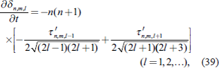
Now, by applying the Galerkin method to the governing equations, the time-derivatives of δ_{n, m, l}, ζ_{n, m, l}, τ̄_l, τ^′_{n, m, l}, and s_{n, m} are determined. Letting the right-hand sides of (1)–(4) be expressed formally as F_δ (λ, μ, σ, t), F_ζ (λ, μ, σ, t), F_τ (λ, μ, σ, t), and F_s (λ, μ, t), respectively, the time-derivatives of δ_{n, m, l}, ζ_{n, m, l}, τ̄_l, and s_{n, m} are determined as follows:   

  

  

  

Here, ⟨·⟩ is the global mean, whose operation is determined as follows:   

On the other hand, by considering that the expansion of τ^′_{n, m, l} is multiplied by σ, the time-derivative of τ^′_{n, m, l} is determined as follows:   

Here, (22) is a simultaneous linear equation for , where B_ll′ is defined as,   

Now, by using the following equations for the Legendre polynomials,   

and the orthogonal relation (16), the components of B_ll′ can be expressed as   

In the matrix form, (B_ll′) can be expressed as follows:   

This is a pentadiagonal symmetric matrix.

Calculations of σ-derivatives in (3), (5), and (6) can be done by noting that   

and the following formula for the derivative of the Legendre polynomial,   

Furthermore, in the calculations of (9) and (10), the definite integrals of the Legendre polynomial should be calculated. These integrals can be calculated as follows. Firstly, integrating both sides of the following equation,   

we obtain,   

By using (25), the following equations are obtained:   

  

By using (26) and (27), we can calculate the definite integrals of the Legendre polynomial in evaluating (9) and (10).

3.1 Transform method

In the equations (18)–(22) that determine the time-derivatives of the dependent variables, the transform method is used to evaluate the integral on the right-hand side. That is, we introduce grid points in the horizontal direction as, (λ_i, μ_j) (i = 1, 2, ..., I; j = 1, 2, ..., J) and grid points in the the vertical direction as, σ_k (k = 1, 2, ..., K), to calculate the integral on the right-hand side by summing the weighted grid values.

For example, the right-hand side of (18) is calculated as follows:   

Here, are the Gaussian nodes, which are defined as zero points (sorted in ascending order) of P_J (μ). The grid points in the vertical direction, σ_k (k = 1, 2, ..., K), are defined as σ_k = (1 − η_k)/2 (k = 1, 2, ..., K), where, η_k (k = 1, 2, ..., K) are zero points (sorted in ascending order) of P_K (η). Also, w_j and W_k are the Gaussian weights, which are defined as follows:   

  

respectively. In the σ-integrals appearing in (18)–(20) and (22), the integrands are 3L-degree polynomials of σ except for the Τ̄(σ) part. This fact can be confirmed as follows. In (1)–(10), u, v, ζ, δ, τ′, τ̄, τ, and Φ′ are L-degree polynomials of σ. Furthermore, since s does not depend on σ, C is also an L-degree polynomial of σ, and from this, it becomes clear that σ̇ is the product of σ and an L-degree polynomial of σ. Thus, A and B are 2L-degree polynomials of σ, and from this, it becomes clear that the right-hand sides of (1)–(3) are 2L-degree polynomials of σ. This confirms the statement above. To avoid the aliasing error, we should set K so that 2K − 1 ≥ 3L is satisfied. That is, since the Gauss-Legendre quadrature formula is used in the vertical direction as well as in the horizontal direction, the choice of the grid points (σ_k) in the vertical direction is automatically determined. Although this may seem a disadvantage in the sense that it lacks flexibility in the way the grid points are chosen, it can be regarded as an advantage in that the optimal grid points for accuracy are automatically determined. Since the Gaussian nodes tend to be dense near the boundary, the grid points (σ_k) are dense near σ = 0, 1. For example, when K = 20, (σ_k) = (0.997, 0.982, 0.956, 0.920, 0.873, 0.818, 0.755, 0.687, 0.614, 0.538, 0.462, 0.386, 0.313, 0.245, 0.182, 0.127, 0.0804, 0.0439, 0.0180, 0.00344) in three significant digits. When K is large, 1 - σ₁ = σ_K ≈ 1.4 × K⁻² and σ₁ − σ₂ = σ_K−1 − σ_K ≈ 6.1 × K⁻² in a rough approximation. Dense grid points near σ = 1 correspond to the increase of the number of grid points in the lower layer of the atmosphere. Conversely, the densification of the grid points near σ = 0 does not necessarily mean that the grid points are dense in the upper atmosphere if we consider the logarithmic pressure coordinate. On the treatment of the basic temperature field, Τ̄(σ), we can give its value and its σ -derivative on the grid points since it appears only in the evaluation of the integral.

4. Semi-implicit time-integration

We denote the vector that formally lumps all of the expansion coefficients (δ_{n, m, l}, ζ_{n, m, l}, τ̄_l, τ′_{n, m, l}, s_{n, m}) together as u. Then, the time-evolution equations (1)–(4) are expressed formally as follows:   

where L is the linear operator for gravity wave propagation (to be defined later) and f (u) is a nonlinear operator that summarizes the other remaining terms. Now, following Durran and Blossey (2012), we consider the use of IMEX (Implicit-Explicit Multistep Methods) for time-integration. Among the IMEX methods, we will use the combination of AM2*/AX2*. Then the scheme of time-integration can be expressed as follows:   

Here, qⁿ is the numerical approximation to u at time nΔt, and Δt is the time step. The specific values of the coefficients are as follows:   

In the actual time evolution, (32) is transformed to the following form of a simultaneous linear equation:   

and it is solved for qⁿ⁺¹. Here, I is the identity matrix. In the following, we will describe the time-evolution corresponding to the linear operator L. Because the explicit matrix form of L is not easily constructed, we derive how to obtain Lq from given q = (δ_{n, m, l}, ζ_{n, m, l}, τ̄_l, τ^′_{n, m, l}, s_{n, m}) as a procedure. We linearize the time-evolution equations (1)–(4) with the basic field being the isothermal stationary atmosphere at the temperature T_0* used in the nondimensionalization. Note that the choice of the value of T_0* affects the behavior of the semi-implicit time-integration. We will set T_0* = 300 K in the benchmark calculations shown in the next section. If we also neglect the effect of the rotation of the sphere, the resulting linearized equation can be expressed as follows:   

  

  

Here, the evolution equation for ζ is omitted because it does not evolve in time in this linearization. Now, considering the expansions of the forms (11)–(14) and applying the Galerkin formulation to (35)–(37) similarly as shown in (18)–(22), we obtain the following by using (23), (26), and (27):   

  

  

  

  

Therefore, if we define the (L + 1) × L matrix (A_ll′) as   

  

(38)–(41) can be expressed as follows:   

  

The elements of the matrix (A_ll′) can be expressed as follows:   

Using (45), (46), and (42), the procedure to obtain Lq from given q is described as follows. The components of Lq corresponding to δ_{n, m, l} and s_{n, m} are directly obtained by calculating the right-hand sides of (45) and (42). The components of Lq corresponding to τ^′_{n, m, l} are obtained by solving the simultaneous linear equation of (46) for ∂τ^′_{n, m, l}/∂t. Conversely, the components of Lq corresponding to ζ_{n, m, l} and τ̄_l are zeros since the system of linearized equations (45), (46), and (42) contains neither ∂ζ_{n, m, l} /∂t nor ∂τ̄_l /∂t.

Now, denoting the components of the whole right-hand side of (34) corresponding to δ_{n, m, l}, τ^′_{n, m, l}, and s_{n, m} by R_{δn, m, l}, R_{τ^′n, m, l}, and R_{sn, m}, respectively, the simultaneous linear equation (34) to be solved can be expressed as follows:   

  

  

  

Here, the solution (δ_{n, m, l}, τ^′_{n, m, l}, s_{n, m}) of this simultaneous linear equation corresponds to qⁿ⁺¹ in (34). For the components of ζ_{n, m, l} and τ̄_l that do not appear here, since the corresponding rows and columns of L are zero, we do not need to solve a simultaneous linear equation for these components, but we should simply calculate the corresponding components of the right-hand side of (34). Now, let us consider the procedure for solving the simultaneous equation (48)–(50) in the following steps. First, substituting (50) into (48) and eliminating s_{n, m}, we can derive the following equation by setting l = 0.   

Solving this for δ_{n, m, 0}, we obtain,   

Thus, including the cases of l ≥ 1, δ_{n, m, l} can be expressed as,   

Substituting the expression (54) into (49), we get   

If we introduce (C_{n, ll′}) as   

(55) can be expressed as follows:   

This is now a simultaneous linear equation for τ^′_{n, m, l′} only. The (C_{n, ll′}) defined by (56) is an L × L matrix for each n. By denoting as b_n = 1/[1 + (ν₁Δt)²n (n + 1)], the components of (C_{n, ll′}) are calculated as follows:   

The matrix representation of (C_{n, ll′}) is as follows:   

This is an L × L pentadiagonal symmetric matrix. In the left-hand side of (57), (B_ll′) is also an L × L pentadiagonal symmetric matrix, so that the entire coefficient matrix of τ^′_{n, m, l′} is also an L × L pentadiagonal symmetric matrix. Thus, τ^′_{n, m, l} can be obtained by solving the simultaneous linear equations with an L × L pentadiagonal diagonal symmetric matrix as the coefficient matrix for each (n, m). From the obtained τ^′_{n, m, l}, we can obtain δ_{n, m, l} by using (54), and from the obtained δ_{n, m, 0}, s_{n, m} can be obtained by (50).

We have now formulated the procedure for time-integration based on (32). However, since (32) is a three-step method, it is necessary to perform time-integration by some other means for two steps from the initial condition. Since the scheme (32) is a second-order scheme, the first two steps must also be calculated by a second-order scheme (or a higher-accuracy scheme). Here, for simplicity, we propose to integrate (31) with the following split-step method. First, the time-evolution by the operator L is done by using the implicit trapezoidal scheme for the time period of Δt/2. Then, the time-evolution by the operator f (u) is done by using Runge–Kutta method of second or higher order for the time period of Δt. Finally, the time-evolution by the operator L is done by using the implicit trapezoidal scheme again for the time period of Δt/2. This maintains the second-order accuracy in the time direction. In the present manuscript, we use a third-order three-stage scheme to consider the stability of the gravity-wave component. Since the time-evolution of the part of the implicit trapezoidal scheme is a time-evolution of 1/2 step, the scheme is expressed as follows:   

Thus, we should solve the following simultaneous linear equation:   

Since the coefficient matrix appearing on the left-hand side of (61) is simply the one that replaces the value of ν₁ used in the procedure below (48) with 1/4 instead of 3/4, the solution for q^n+1/2 can be calculated using the the same procedure. Thus, the whole calculation procedure, including the Runge-Kutta part and writing (61) again, is summarized as follows:   

  

  

4.1 Treatment of dissipation terms

As in the setting of Held and Suarez (1994), which we will discuss later, we often include a dissipation term in the right-hand side of (31) as follows:   

Here, Γ is the matrix representing the dissipation effect, which we assume to be a diagonal matrix. It is of course possible to combine the effects of this term into the linear operator L. In that case, however, the shape of the coefficient matrix becomes more complicated when the semi-implicit method described above is applied. Thus, in the present manuscript, we propose the following method. Introducing the vector-valued function v (t) as   

we can derive the following equation from (65).   

Let us apply AM2*/AX2* scheme to perform the timeintegration of this differential equation for v. Denoting the numerical approximation of v at time nΔt as rⁿ, the scheme corresponding to (32) can be expressed as follows:   

Multiplying e^{−(n+1)ΔtΓ} from the left to both sides of this equation and noting that e^−nΔtΓrⁿ = q_n, (68) can be rewritten as follows:   

Therefore, comparing (69) and (32), we can see that the inclusion of the dissipation term means that we only need to apply attenuation when using values from past time steps. Note that in this case, the first two steps should also be changed from (62)–(64). (62) and (64) should be changed to   

and   

respectively.

5. Benchmark experiments and accuracy assessment

In this section, we implement the three-dimensional spectral formulation of the primitive equations described so far as a numerical model, and check that it gives reasonable numerical solutions by using benchmark experimental settings proposed in previous studies. To check the effect of using the spectral method also in the vertical direction, we investigate the dependence of the computational accuracy on the discretization degrees of freedom in the vertical direction.

In the numerical calculations presented in this section, ispack-3.1.0 (https://www.gfd-dennou.org/arch/ispack/), which is designed based on Ishioka (2018), is used for the transform method described in Section 3.1.

5.1 Benchmark experiment based on Polvani et al. (2004)

First, we calculate the time-evolution of baroclinic disturbances, which grow by baroclinc instaility of a mid-latitude zonal jet, based on the benchmark setting of Polvani et al. (2004).

In the benchmark setting of Polvani, et al. (2004), a baroclincally unstable mid-latitude zonal jet and a zonal temperature field, which is in the thermal wind balance with the jet, are given as the initial basic state. A Gaussian-like initial temperature disturbance is added to the unstable basic state, and the time-evolution of the whole system, including the growth of baroclinic disturbances, is calculated. For details of the benchmark settings, see Polvani et al. (2004). Figure 1 shows the time-evolution of the temperature field on the σ = 0.975 surface, corresponding to Fig. 2 in Polvani et al. (2004). While the horizontal truncation wavenumber is T341 and the number of the vertical levels for the finite difference scheme in the σ-coordinate is 20 for the calculation of Fig. 2 in Polvani et al. (2004), the horizontal truncation wavenumber is T170 and the vertical truncation wavenumber is 13 (the number of the vertical grids is 20) for the calculation of Fig. 1 in the present manuscript. The time step also differs: Δt = 150 s in Polvani et al. (2004) and Δt = 600 s in the present manuscript. Comparing Fig. 1 in the present manuscript and Fig. 2 in Polvani et al. (2004) shows almost perfect agreement on the fine structure of the contours of the temperature field at time t = 12 days. It is worth noting that the number of the vertical levels in the calculation for Fig. 2 in Polvani et al. (2004) is 20, but the vertical truncation wavenumber for the calculation of Fig. 1 in the present manuscript is 13. This means that although the vertical degrees of freedom used in the threedimensional spectral model here is smaller than that used in Polvani et al. (2004), the development pattern of the baroclinic disturbance can be calculated with almost the same accuracy using the three-dimensional spectral model.

Fig. 1.

Temperature fields on the σ = 0.975 surface at time t = 4, 6, 8, 10, and 12 days (unit is K) in the course of time-evolution of the growth of the baroclinic disturbance calculated on the basis of the benchmark setting in Polvani et al. (2004) by using the three-dimensional spectral model developed in the present manuscirpt. Contour interval is 2.5 K. The horizontal axis is longitude and the vertical axis is latitude. The time is shown in the upper right corner of each panel. The horizontal truncation wavenumber is T170 (512 × 256 grids), the vertical truncation wavenumber is 13 (20 grids), and the time step Δt is 600 s.

5.2 Benchmark experiment based on Held and Suarez (1994)

Next, to check the mean field of long time-evolution, meridional distribution of the zonal mean temperature field and the zonal mean zonal wind field for 1000-day mean from the 200th day of time-evolution based on the benchmark setting of Held and Suarez (1994) are calculated by using the three-dimensional spectral model developed in the present manuscript and shown in Fig. 2. The top panel of Fig. 2 corresponds to Fig. 1c in Held and Suarez (1994), and the bottom panel of Fig. 2 corresponds to Fig. 2 in Held and Suarez (1994).

Fig. 2.

Zonal mean field averaged over 1000 days from t = 200 days to t = 1200 days in the time-evolution with the benchmark setting based on Held and Suarez (1994). The horizontal axis is latitude and the vertical axis is σ . Top panel: zonal mean temperature field (K). Contour interval is 5K. Bottom panel: zonal mean eastward wind field (m s⁻¹). Contour interval is 4 m s⁻¹. In the calculation of the time-evolution, the horizontal truncation wavenumber is T85 (256 × 128 grids), the vertical truncation wavenumber is 13 (20 grids), and the time step is 720 s.

The calculation of Held and Suarez (1994) is done using the finite difference method with 144 × 72 grids or a spectral method with T63 for the discretization in the horizontal direction and the finite difference method with 20 levels in the vertical direction. For the calculation of Fig. 2 in the present manuscript, the horizontal truncation wavenumber is T85, the vertical truncation wavenumber is 13 (20 grids), the time step Δt is 720 s, and the initial disturbance is the same Gaussian-like temperature disturbance as that is used in Polvani et al. (2004). In this long-time average statistical equilibrium state, the meridional structures of the zonal mean temperature and zonal mean zonal wind fields are in good agreement with those obtained in Held and Suarez (1994), even though the vertical truncation wavenumber of the three-dimensional spectral model is 13, which is a small number of degrees of freedom, as in the case of the previous subsection.

5.3 Benchmark experiment based on Jablonowski and Williamson (2006)

At the end of the benchmark tests, we perform numerical calculations of the growth of baroclinic disturbances according to the settings proposed by Jablonowski and Williamson (2006). This setup is similar to that of Polvani et al. (2004), but with a north-south symmetric zonal wind and temperature fields, and the smoothness of the basic field is considered. The initial disturbance is a Gaussian-like distribution in the eastward wind field in the northern hemisphere. Figure 3 shows the surface pressure field on day 9 in the time-evolution calculated on the basis of this benchmark setting, with the horizontal truncation wavenumber of T170 (512 × 256 grids), the vertical truncation wavenumber is 17 (26 grids), and the time step is 300 s. This figure corresponds to Fig. 7a in Jablonowski and Williamson (2006). However, in the present manuscript, the horizontal diffusion term for the sponge-like effect in the upper layer, which is added in Jablonowski and Williamson (2006), is not added. By comparing Fig. 7a of Jablonowski and Williamson (2006) with Fig. 3 of the present manuscript, we can see that there is a slight difference in the pattern of the contour lines of 1000 hPa because the position of the 1000 hPa contour lines can vary greatly even with very small deviations from the basic field. Nevertheless, the contours at other levels show almost perfect agreement down to the fine structure. It is still worth mentioning that the number of the vertical levels in the calculation for Fig. 7a in Jablonowski and Williamson (2006) is 26, but the vertical truncation wavenumber for the calculation of Fig. 3 in the present manuscript is 17. This means that although the vertical degrees of freedom used in the three-dimensional spectral model here is smaller than that used in Jablonowski and Williamson (2006), the development pattern of the baroclinic disturbance can be calculated with almost the same accuracy by the three-dimensional spectral model.

Fig. 3.

The surface pressure field on day 9 (unit is hPa) in the course of time-evolution of the growth of the baroclinic disturbance calculated on the basis of the benchmark setting in Jablonowski and Williamson (2006) by using the three-dimensional spectral model developed in the present paper. Contour interval is 10 hPa. The horizontal axis is longitude, and the vertical axis is latitude. The maximum value in this figure is 1019.73 hPa [at (λ, φ) = (231.33°, 49.47°)]. The minimum value is 942.03 hPa [at (λ, φ) = (208.13°, 61.40°)]. The horizontal truncation wavenumber is T170 (512 × 256 grids), the vertical truncation wavenumber is 17 (26 grids), and the time step is 300 s.

Next, we examine the convergence of the numerical solution for the three-dimensional spectral model with changing the vertical truncation wavenumber. Figure 4 shows the dependence of the error of the surface pressure field on the vertical truncation wavenumber L for days 1, 5, 9, 11, and 12, measured in l₂ norm. The result at L = 170 (K = 256) is taken as the true value here and we define the difference from it as the error. The horizontal truncation wavenumber is T85 (256 × 128 grids), and the time step is 150 s. Here, the reason why the small time step is used is to ensure the stability of the calculation even in the case of L = 170 (K = 256). In Fig. 4, the horizontal places of the markers indicate the values of the vertical truncation wavenumber L used in the time-integrations (L = 10, 11, 12, 13, 14, 15, 16, 17, 21, 42, and 85). The corresponding number of the vertical grids, K, is K = 16, 18, 20, 20, 22, 24, 26, 26, 32, 64, and 128, respectively. If the error of the surface pressure measured in the l₂ norm is expressed as ∈, the dependence of ∈ on L is expressed approximately as ∈ ∼ L⁻¹ for days 1 and 5. We believe that this is caused by horizontal propagation of Lamb wave modes excited by the initial disturbance until baroclinic disturbances develop due to baroclinic instability. As shown in Appendix A.4, in this three-dimensional spectral model, the error of phase speed of Lamb wave modes is roughly proportional to L⁻¹. Thus, as Lamb wave modes excited by the initial disturbance propagate horizontally, the influence of phase speed difference increases with time and the error of surface pressure also increases; hence, the error is considered to be approximately proportional to L⁻¹. Conversely, on day 9, in the region where L is small (L = 10 to L = 15) the L-dependence of ∈ is clearly higher power curve than L⁻¹ (∈ ∼ L⁻⁴), and on days 11 and 12, a still higher power dependence (∈ ∼ L⁻⁶) is observed in the region from L = 10 to L = 17. This is because after day 9, as seen in Fig. 3, baroclinic disturbances are sufficiently developed and the error included in the evaluation of the advection effect due to the vertical velocity becomes larger than that of the phase speed of the initially excited Lamb wave modes. Since the vertical discretization error affects the evaluation of the vertical advection largely, it can be interpreted that using the spectral method in the vertical direction makes the error decrease rapidly as L is increased.

Fig. 4.

The dependence of l₂ error of the surface pressure field (vertical axis. unit is hPa) on the vertical truncation wavenumber L (horizontal axis) at days 1, 5, 9, 11, and 12 in the time-evolutions of baroclinic disturbances on the basis of the benchmark setting of Jablonowski and Williamson (2006). Both the axes are in logarithms. The result at L = 170 (K = 256) is taken as the true value here, and we define the difference from it as the error. The horizontal places of the markers indicate the values of the vertical truncation wavenumber L used in the time-integrations (L = 10, 11, 12, 13, 14, 15, 16, 17, 21, 42, and 85). The corresponding number of the vertical grids, K, is K = 16, 18, 20, 20, 22, 24, 26, 26, 32, 64, and 128, respectively. The number of days is indicated at the left end of the line connecting the markers. The time-integrations are done with the horizontal truncation wavenumber of T85 (256 × 128 grids) and the time step of 150 s.

In Fig. 4, the error from the initial disturbance itself has a certain magnitude before the development of the disturbance due to baroclinic instability. Thus, the effect of vertical resolution on the improvement of accuracy at the timing of the development of the baroclinic disturbances is somewhat obscured. To resolve this point, we perform time-integrations again on the basis of the benchmark setting of Jablonowski and Williamson (2006), but where the amplitude of the initial disturbance is set to 1/1000. Figure 5 shows the surface pressure field on day 19 in such a setup, with the horizontal truncation wavenumber of T85 (256 × 128 grids), the vertical truncation wavenumber of 170 (256 grids), and the time step of 150 s. Since the amplitude of the initial disturbance is reduced, the development of the baroclinic disturbances is delayed when compared with the case of Fig. 3. However, after a sufficient amount of time has elapsed, well-developed low pressure systems can be seen. Figure 6 shows the convergence of the numerical solution with changing the vertical truncation wavenumber for the case where the amplitude of the initial disturbance is set to 1/1000 of the standard value, as in Fig. 4. Since the development of the baroclinic disturbances is delayed in comparison with the case of Fig. 4, the dependence of the error on the vertical truncation wavenumber L is shown for days 1, 9, 11, 13, 15, 17, 19, and 21. The time-integrations are done with the horizontal truncation wavenumber of T85 (256 × 128 grids) and the time step of 150 s. In Fig. 6, on days 1 and 9, the dependence of ∈ on L is expressed approximately as ∈ ∼ L⁻¹, which is the same as days 1 and 5 in Fig. 4. We believe that this is caused by Lamb wave modes directly excited by the initial disturbance similarly as on days 1 and 5 in Fig. 4. Nevertheless, in Fig. 6, the amplitude of the initial disturbance is set to 1/1000, so that the ∈ on day 1 in Fig. 6 is almost 1/1000 of that on day 1 in Fig. 4. In Fig. 6, on day 11, in the region where L is small (L = 10 to L = 21) the L-dependence of ∈ is clearly higher power curve than L⁻¹ (∈ ∼ L⁻³) as seen on day 9 in Fig. 4. After day 13, when the baroclinic disturbances develop, the power of the power-law dependence becomes higher, and on day 17, the dependence is ∈ ∼ L⁻⁶ in the range of L = 10 to L = 42. Thus, these time-integrations with the reduced amplitude of the initial disturbance clearly shows that in the development of baroclinic disturbances, using the spectral method in the vertical direction makes the error decrease rapidly as L is increased. In Fig. 6, however, the ∈ becomes large even when L is large (L = 42, 85) in days 19 and 21. We believe that this is due to the increase of high-wavenumber components in the vertical direction, which are produced by nonlinear effects enhanced by the growth of the baroclinic disturbances.

Fig. 5.

Same as Fig. 3 except that the amplitude of the initial disturbance is 1/1000 of that used for the computation of Fig. 3, and this figure is on day 19. Contour interval is 10 hPa. The maximum value in this figure is 1022.82 hPa [at (λ, φ) = (29.53°, 48.33°)], The minimum value is 950.45 hPa [at (λ, φ) = (50.63°, 63.73°)]. The horizontal truncation wavenumber is T85 (256 × 128 grids), the vertical truncation wavenumber is 170 (256 grids), and the time step is 150 s.

Fig. 6.

Same as Fig. 4 except that the amplitude of the initial disturbance is 1/1000 of that used for the computation of Fig. 4. The times are days 1, 9, 11, 13, 15, 17, 19, and 21.

6. Summary and discussion

In the present manuscript, we have proposed to use a three-dimensional spectral method for the GCM dynamical core on the basis of the primitive equations, which uses the spectral method not only in the horizontal direction but also in the vertical direction, where the Legendre polynomial expansion is used and the time-evolution equations of the expansion coefficients are determined by the Galerkin method. We have shown that the semi-implicit time-integration can be computed more efficiently with the vertical discritization formulation proposed in the present manuscript. This is an improvement compared with the previous study by Machenhauer and Daley (1974), where the Legendre polynomial expansion was also used in the vertical direction. Using the numerical model implemented based on the proposed three-dimensional spectral method, modern benchmark numerical experiments with the settings of Polvani, et al. (2004), Held and Suarez (1994) and Jablonowski and Williamson (2006) have been performed to show that the numerical results are consistent with those of previously developed numerical models and to show that there is no numerical instability caused by the use of the three dimensional spectral method. Also, in Section 5.3, we have evaluated the convergence of the numerical solution for different truncation wavenumbers in the vertical direction. It has been shown that the error decreases rapidly as the vertical truncation wavenumber increases, which is a characteristic of the spectral method. This is an advantage over the finite difference method, which is often used in existing numerical models. In fact, in the benchmark calculations shown as Figs. 1–3, the numbers of the vertical grids are set to be the same as the numbers of the vertical levels in previous studies; however, each vertical truncation wavenumber is approximately 2/3 of the number of the vertical grids. This means that a numerical solution with high-accuracy is obtained with a small number of degrees of freedom. The fact that fewer degrees of freedom are needed is not only an advantage in data storage, but also it has the advantage of reducing the size of the matrix in which the eigenvalue problem should be solved when calculating the flow stability.

If we compare the three-dimensional spectral method proposed in the present manuscript with ordinary numerical models that uses the finite difference method in the vertical direction, some disadvantages, of course, can be considered. One of them is the computational cost in transforming between the coefficients of the Legendre polynomial expansion and the grid values. If the vertical truncation wavenumber is L and the horizontal truncation wavenumber of the spherical harmonic expansion is M, the cost of the vertical transform required per one time step is estimated to be O (L²M²). When the finite difference method is used in the vertical direction, the computational cost of the vertical calculation is O (KM²) if the number of the vertical levels is K. Thus, the comparison reduces to the comparison of O (L²) and O (K). Since K ∼ L, the three-dimensional spectral method looks worse in terms of the computational cost. However, since the computational cost of the horizontal transform is estimated to be O (LM³), the computational cost of the vertical transform becomes a small fraction of the total computational cost in the situation where the horizontal truncation wavenumber is sufficiently large when compared with the vertical truncation wavenumber (L ≪ M). Therefore, the use of the spectral method in the vertical direction is not a big disadvantage unless the truncation wavenumber in the vertical direction is larger than the that in the horizontal direction.

The second possible disadvantage is that the spectral method proposed in the present manuscript does not strictly guarantee the conservation of the total energy. This is because in the formulation of the timeevolution of the temperature disturbance field (22), the weighting function is set to be σP_l (1 − 2σ), which is the same function as used in the expansion according to the Galerkin method. If we set the weighting function as P_l (1 − 2σ), we can satisfy the total energy conservation. In this case, since the weight is set to 1/σ as in the original Galerkin method and this means that the weight of the upper atmosphere is relatively increased and the weight of the lower atmosphere is relatively decreased, the benchmark calculation shows that the accuracy of the calculation in the lower atmosphere is lower than that of the one proposed in the present manuscript (not shown). In that case, we also lose the property that the matrix to be computed is a band matrix in the formulation of the semi-implicit method. In actual GCM calculations, the effects of forcing and dissipation are introduced; so, even if the discretized system does not strictly satisfy the total energy conservation, it does not seem to be a big disadvantage unless it leads to any numerical instability.

The third possible disadvantage is that the vertical discretization grids are automatically set by the Gaussian node η_k, and there is no freedom in the vertical grid setting as in the finite difference method. However, this point can be regarded as an advantage in that the “optimal” vertical grids are automatically determined once the number of the vertical grids is determined, without having to worry about how to set the vertical grids. Additionally, in the case of the finite difference method, the existence of computational mode can be a problem when the Lorenz grid is used in the vertical direction (Arakawa and Konor 1996). In the spectral method proposed in the present manuscript, however, there is no such computational mode (see Appendix A.4). This point can also be considered as one of the advantages of the spectral method proposed in the present manuscript.

As described above, the discretization of the primitive equations by the three-dimensional spectral method proposed in the present manuscript has advantages over the conventional discretization using the finite difference method in the vertical direction in terms of accuracy and other factors. Particularly, it is useful for theoretical studies when a small number of degrees of freedom are used. As an extreme form of such an application, a “toy” model equation is derived for the case where the vertical degree of freedom is reduced to the minimum in Appendix B.

Acknowledgments

We thank two anonymous reviewers for their helpful comments. This work was supported by JSPS KAKENHI Grant Numbers 20K04061. This work was also supported by MEXT as “Program for Promoting Researches on the Supercomputer Fugaku” (Toward a unified view of the universe: from large scale structures to planets, JPMXP1020200109) and “Exploratory Challenge on Post-K computer” (Elucidation of the Birth of Exoplanets [Second Earth] and the Environmental Variations of Planets in the Solar System).

This work used computational resources of the K computer and supercomputer Fugaku provided by the RIKEN Center for Computational Science through the HPCI System Research Project (Project ID: hp160254, hp170225, hp180199, hp190170, hp200124, hp210164).

The GFD-DENNOU Library (https://www.gfddennou.org/arch/dcl/) was used to draw the figures.

Appendix A: Pseudo-hyper-viscosity

The primitive equations in the σ -coordinate system treated in the present manuscript use the boundary condition at σ = 0, which means that the region that extends to infinite height is treated as a finite σ region. Thus, if we consider a wave propagating vertically upward, the wave that should have propagated infinitely upward and left the region will be artificially reflected back into the region. This means that the time-evolution of the wave cannot be treated correctly. This situation is the same as that of the finite difference method, even if the spectral method is used in the vertical direction. In the case of the finite difference method, if it is possible to impose a radiative boundary condition, it may be done, but it is difficult to do so except in special cases where the waves are monochromatic. Therefore, a damping region (sponge layer) of a certain thickness is set near the upper boundary of the computational domain to suppress the reflection by absorbing the upward propagating waves. Nevertheless, if the damping ratio and the thickness of the sponge layer are not set properly, the wave absorption will be insufficient and reflected waves will be generated. When using the spectral method by projecting a geometrically infinite domain onto a finite domain, as in the present manuscript, the effect corresponding to a sponge layer can be obtained by introducing the pseudo-hyper-viscosity (Ishioka 2008). We show below that such pseudo-hyper-viscosity can also be introduced when the spectral method is used in the vertical direction as in the present manuscript.

A.1 Description of gravity wave propagation in this system

As in the case where the semi-implicit method is introduced in Section 4, we linearize the time-evolution equations (1)–(4) with the basic field being the isothermal atmosphere at the temperature T_0* used in the nondimensionalization and with neglecting the effect of the rotation of the sphere. For further simplification, we assume here that the horizontal geometry is not a sphere but a plane. We use Cartesian coordinates (x, y) of the plane, and assume the field variables to be uniform in the y-direction. In this case, we nondimensionalize the length scale using an appropriate length X_* in the x-direction. If we assume that a uniform flow U > 0 is blowing in the x-direction, the linearized equation using it as the basic field can be expressed as follows (here, we consider the effect of the topography).   

  

  

Here, the vorticity ζ is omitted in this linearization because it does not evolve in time. Now, in the x-direction, we consider a wave solution with dimensionless wavenumber k > 0 and and express it as follows:   

  

  

  

Then, from (72)–(74), we obtain   

  

  

This equation describes the propagation of internal gravity waves forced by the bottom topography. This equation is a little complicated because it is written in the σ -coordinate. However, if we impose the radiative boundary condition and consider steady state with a positive vertical group velocity, we obtain the following solution (the derivation process is omitted):   

Here, we define that z = − ln σ and   

Note that m is used as the vertical wavenumber, not the longitudinal wavenumber in this appendix. Here, we also impose that for a solution with a positive vertical group velocity to exit. In this case, δ _s is determined as follows:   

A.2 When discretized by the spectral method

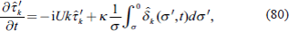
Similarly as (11) and (13), we expand δ̂_k (σ, t) and τ̂^′_k (σ, t) appearing in (79)–(81) as follows:   

  

In this case, applying the Galerkin formulation to (79)–(81) in the same way as when we derived (45), (46), and (42), we obtain the following:   

  

  

(87)–(89) can be transformed as follows:   

  

  

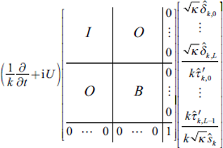
The matrix representation of (90)–(92) is as follows:   

Here, B is a (L + 1) × (L + 1) matrix whose (l, l′) component is B_ll′, and A is a (L + 1) × L matrix whose (l, l′) component is A_ll′ (the subscripts l and l′ are starting from 0). The square matrix appearing on the left-hand side of (93) is a symmetric matrix, and the square matrix on the right-hand side is a skew-symmetric matrix.

A.3 Steady-state solution in the discretized system and the introduction of pseudo-hyper-viscosity

In the system discretized by the spectral method, (93), we consider a stationary solution. In the right-hand side of (93), we set   

Then, the stationary solution is obtained by solving a linear simultaneous equation, which is derived by setting ∂/∂t = 0 in (93). Corresponding to (δ̂_{k, l}) in the stationary solution, the σ distributions of the imaginary part of δ̂_k (σ) for U = 0.05 and U = 0.1 are shown in Fig. 7. For comparison, the stationary solutions (with the radiative boundary condition) determined by (82) and (84) are plotted together. The amplitude is multiplied by , considering its dependence on σ . Figure 7 clearly shows that the numerical solution differs significantly from the exact solution because of the effect of reflected waves.

Fig. 7.

The σ distribution of the imaginary part of the stationary wave solution without pseudo-hyper-viscosity (multiplied by ). Numerical solution (solid line) and the exact solution for the case with radiative boundary condition (dotted line). Left panel: U = 0.05 case, right panel: U = 0.10 case. The vertical truncation wavenumber is L = 80.

Now, referring to Ishioka (2008), in the right-hand side of (93), we introduce the effect of pseudo-hyperviscosity at the diagonal components of the matrix, which correspond to the divergence components as follows:   

Here, (ν_h)_l (l = 0, 1, ..., L) are the coefficients of the pseudo-hyper-viscosity. How to set the values of (ν_h)_l is subject to arbitrariness. If we set   

and calculate the steady-state solution as in Fig. 7, the result is shown in Fig. 8. Thus, by introducing a pseudo-hyper-viscosity, it acts like a sponge layer in the upper atmosphere, where σ is small, and suppresses the reflected waves. By suppressing the reflected waves, a response close to the exact solution is obtained in the lower atmosphere. Using (95) in (94), a strong dissipation on δ in the upper-layer atmosphere like a sponge layer can be explained as follows. Considering (24), the dissipation term in the equation of ∂δ/∂t can be expressed as follows:   

Now, changing the independent variable as , (96) can be rewritten as follows:   

Thus, as z → ∞, a hyper-viscosity of the fifth-order of the Laplacian acts on δ and its coefficient increases roughly in proportion to e^5z. This corresponds to having an effect similar to introducing a sponge layer in the upper layer of the model. We can change the characteristics of the spongy effect by changing the order and coefficients of the pseudo-hyper-viscosity in (95).

Fig. 8.

Same as Fig. 7 except that the numerical solution (solid line) is computed with pseudo-hyper-viscosity.

Now, the introduction of pseudo-hyper-viscosity in the form of (94) means that we add the pseudo-hyper-viscosity term in (87) as follows:   

Here, the pseudo-hyper-viscosity term is the first term on the right-hand side. Furthermore, in the expression for the spherical domain (18), we can add to the right-hand side since the k is replaced by . Note that the pseudo-hyper-viscosity is not added in the benchmark numerical experiments in Section 5. It would be desirable if we had also performed test-case calculations to examine the effects of the pseudo-hyper-viscosity, such as Klemp et al. (2015), in which the model suffers from gravity waves reflecting off the model top. However, this test case appears to be for a nonhydrostatic model, and the intercomparison does not seem directly applicable to our hydrostatic model, and we need to find some appropriate test case to evaluate the effect of the pseudohyper- viscosity. Hence, let us leave this exploration to our future work.

A.4 Eigenvalue problems and the Lamb wave solution

In the linear time-evolution equation discretized by the spectral method (93), setting the rightmost term of the terrain effect to 0, and the basic flow U = 0, we obtain the following eigenvalue problem assuming that the time-dependence is expressed as ∝ e^−iωt:   

Here, c = ω / k. Since the square matrix appearing on the left-hand side of (99) is a positive-definite symmetric matrix and the square matrix on the right-hand side is a skew-symmetric matrix, we can see that the eigenvalues of ic are purely imaginary, so the eigenvalue c corresponding to the phase velocity is eventually a real number. Furthermore, there are no zero eigenvalues associated with the even number of rows (or columns) of the coefficient matrices on the left and right sides in (99). This means that the computational mode that arises when the Lorenz grid is used for the finite difference method in the vertical direction, as described in Arakawa and Konor (1996), does not arise in this formulation of the spectral method. Nevertheless, in the vertical discretization of τ′, if the truncation wavenumber is set to L instead of L − 1, a zero eigenvalue appears. In this sense, it is also desirable to take the truncation wavenumber in the expansion of τ′ as L − 1.

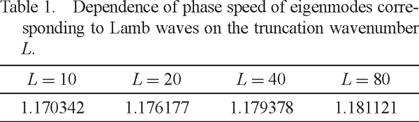
The eigenvalue problem (99) can be solved numerically. The eigenmode that gives the maximum absolute value of eigenvalue c is the one corresponding to the Lamb wave mode. Table 1 shows the maximum absolute value of eigenvalue c for different vertical truncation wavenumber L, and Fig. 9 shows the σ distribution of δ̂_k (σ) for the corresponding eigenmodes. Note that we now set κ = 2/7 and the true value of | c | corresponding to the Lamb wave is, .

Fig. 9.

Dependence of the amplitude of the eigenmode corresponding to the Lamb wave on σ (solid line). The dotted line is for the exact solution of the Lamb wave (σ^−κ). The vertical truncation wavenumber is changed to L = 10, 20, 40, and 80. The value of L is displayed in the upper-right corner of each panel.

Table 1 shows that the eigenvalue of the largest absolute value approaches the true value corresponding to the Lamb wave as the truncation wavenumber L is increased. Correspondingly, from Fig. 9, it can be seen that the vertical structure of eigenmodes approaches that of the Lamb wave solutions up to smaller σ as L increases. Figure 10 shows the L-dependence of the error of the phase velocity from the true value. It can be seen that the error is roughly at the power of L⁻¹.

Fig. 10.

Dependence of the difference between the eigenvalues of the discretized eigenmodes corresponding to the Lamb wave and the exact solution (vertical axis) on L (horizontal axis). The marker indicates the value of L that was used (L = 10, 20, 40, and 80).

Appendix B: Deriving a toy model

As one byproduct of the formulation of the three-dimensional spectral method proposed in the present manuscipt, by setting the truncation wavenumber L in the vertical direction to a small value such as 1 or 2, we can create a “toy” model that is equivalent to the so-called two-level model or three-level model, without having to worry about how to take the grid in the vertical direction or how to set the finite difference scheme. For example, in (11)–(14), if we set as L = 1, then we can obtain a closed system of equations for the time-dependent expansion coefficients, (δ_{n, m, 0}), (δ_{n, m, 1}), (ζ_{n, m, 0}), (ζ_{n, m, 1}), τ̄₀, τ̄₁, (τ^′_{n, m, 0}), and (s_{n, m}). Since we have two degrees of freedom in the vertical direction in this setting, this can be regarded as corresponding to the so-called two-layer model or two-level model. However, in this form, since the system contains the barotropic component of the divergence field (δ_{n, m, 0}) and the logarithm of the surface pressure (s_{n, m}), the Lamb wave modes are supported in the system, which is complicated for a “toy” model. Similar to the two-level model proposed by Kitamura and Matsuda (2004), a “toy” model without the Lamb wave modes and with good symmetry between barotropic and baroclinic modes can be derived as follows.

First, in (11)–(14), we set the truncation wavenumber as L = 1, that is we set the degree of freedom in the vertical direction to 2. However, to exclude the Lamb waves, the barotropic component of the divergence field (δ_{n, m, 0}) and the logarithm of the surface pressure (s_{n, m}) are assumed to be 0 and are removed from the time-evolution. The bottom topography is assumed to be flat and we set as Φ^′_s = 0. Furthermore, for the temperature disturbance τ, we assume that it is symmetric around the middle layer of the atmosphere and use the following expression instead of the expansion form of (13).   

  

Here, the coefficient in (100) is chosen to simplify the subsequent calculations. Noting that in the definition of the present manuscript, the first-order Legendre polynomial P₁ (η) is defined as , we use the following expressions instead of (11) and (12):   

  

  

  

  

That is, δ (λ, μ, σ, t) is expressed using the first baroclinc component δ_c (λ, μ, t) and ζ (λ, μ, σ, t) is expressed by a superposition of the barotropic component ζ_t (λ, μ, t) and the first baroclinc component ζ_c (λ, μ, t).

Now, let us consider the time-evolution equation of δ_c, ζ_t, ζ_c, and τ_c. From the assumptions made in this Section, (1)–(10) simplify to the following:   

  

  

  

  

  

  

Now, using (102), the equation (112) can be expressed as follows:   

Also, using (100), the equation (113) can be expressed as follows:   

Also for (u, v), we separate them into barotropic components (u_t, v_t) and baroclinic components (u_c, v_c) as u = u_t + u_c, v = v_t + v_c. Decomposing the stream function ψ and the velocity potential χ into barotropic components and baroclinic components (χ has only the baroclinc component), we express ζ_t, ζ_c, and δ_c as follows:   

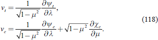
Then, u_t, u_c, v_t, and v_c are expressed as follows:   

  

In this case, considering (102), (104), and (114), the equations (110) and (111) can be written as   

  

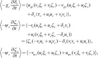
Based on the above preparation, the Galerkin method is used to determine the time-evolution equations of δ_c, ζ_t, ζ_c, and τ_c. That is, by multiplying on both sides of (107), multiplying P₀ = 1 on both sides of (108), multiplying on both sides of (108), and multiplying σ (1 − σ) on both sides of (109), we obtain the followings by integrating them from 0 to 1 for σ.   

  

  

  

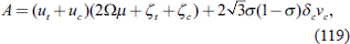
Here, we set ξ_t = 2Ωμ + ζ_t and   

Here, S becomes a static stability measure. Also, for the derivation of (124), the following is used.   

The system of equations derived here, (121)–(124), is very similar to the two-level system of equations derived in Kitamura and Matsuda (2004). The only major difference is that the coefficient on the equivalent of τ_c in parentheses in the third term on the right-hand side of (124) is negative in Kitamura and Matsuda (2004). This is because we consider a boundary condition for the disturbance component of the temperature field τ such that it is 0 for σ = 0, 1, whereas in Kitamura and Matsuda (2004), the disturbance component of the specific volume α is set to be 0 at σ = 0, 1. This reverses the contribution of the disturbance to the static stability of the field. However, this is due to the different structure of the temperature disturbances considered in the very coarse σ discretization. Hence, it is not a matter of which is correct.

Now, in (124), if T̄ is an isothermal basic field independent of σ, then, by (125), we have   

Additionally, let us consider the model temperature distribution of the tropical atmosphere introduced by Stevens et al. (1977) which satisfies the following:   

where Γ is a constant. That is,   

where T̄_s is the value of T̄ at σ = 1. In this case, S is expressed as   

For further simplification, we assume that and ignore the τ_c term in parentheses in the third term on the right-hand side of (124). Then (124) reduces to,   

Now, in the system of (121)–(123) and (126), we show that the energy conservation law holds. If we represent the operation of averaging on the whole sphere by ⟨·⟩, we obtain the following:   

  

Here, we define   

Summing the two equations for the baroclinic components, we get   

If we represent the kinetic energy density as , then finally, we obtain   

Therefore, the energy conservation law in this system is expressed as   

The second term in the left-hand parenthesis corresponds to the available potential energy. Therefore, the system of (121)–(123) and (126) includes baroclinic effects and inertial-gravity modes on a rotating sphere, and the system has the energy conservation law written in the second order of the field variables. This system can be regarded as a kind of “toy” model, following Lindborg and Mohanan (2017), and we will call it the “baroclinic toy-model equation”.

References

•  Arakawa,  A., and  C. S.  Konor, 1996: Vertical differencing of the primitive equations based on the Charney-Phillips grid in hybrid σ-p vertical coordinates. Mon. Wea. Rev., 124, 511-528.
•  Boljka,  L.,  T. G.  Shepherd, and  M.  Blackburn, 2018: On the coupling between barotropic and baroclinic modes of extratropical atmospheric variability. J. Atmos. Sci., 75, 1853-1871.
•  Durran,  D. R., 2010: Numerical Methods for Fluid Dynamics: With Applications to Geophysics. Springer, 532 pp.
•  Durran,  D. R., and  P. N.  Blossey, 2012: Implicit-explicit multistep methods for fast-wave-slow-wave problems. Mon. Wea. Rev., 140, 1307-1325.
•  Lindborg,  E., and  A. V.  Mohanan, 2017: A two-dimensional toy model for geophysical turbulence. Phys. Fluids, 29, 111114, doi:10.1063/1.4985990.
•  Held,  I. M., and  M. J.  Suarez, 1994: A proposal for the intercomparison of the dynamical cores of atmospheric general circulation models. Bull. Amer. Meteor. Soc., 75, 1825-1830.
•  Ishioka,  K., 2008: A spectral method for unbounded domains and its application to wave equations in geophysical fluid dynamics. IUTAM Symposium on Computational Physics and New Perspectives in Turbulence.  Kaneda,  Y. (ed.), Springer, Dordrecht, 291-296.
•  Ishioka,  K., 2018: A new recurrence formula for efficient computation of spherical harmonic transform. J. Meteor. Soc. Japan, 96, 241-249.
•  Jablonowski,  C., and  D. L.  Williamson, 2006: A baroclinic instability test case for atmospheric model dynamical cores. Quart. J. Roy. Meteor. Soc., 132, 2943-2975.
•  Kitamura,  Y., and  Y.  Matsuda, 2004: Numerical experiments of two-level decaying turbulence on a rotating sphere. Fluid Dyn. Res., 34, 33-57.
•  Klemp,  J. B.,  W. C.  Skamarock, and  S.-H.  Park, 2015: Idealized global nonhydrostatic atmospheric test cases on a reduced-radius sphere. J. Adv. Model. Earth Syst., 7, 1155-1177.
•  Kuroki,  Y., and  S.  Murakami, 2015: Development of hydrostatic 3-dimensional spectral model using Chebyshef polynomial expansion in the vertical direction. Proceedings of the MSJ Spring Meeting 2015, P434 (in Japanese).
•  Machenhauer,  B., and  R.  Daley, 1974: Hemispheric spectral model. Modelling for the First GARP Global Experiment. GARP Publication Series, No. 14, World Meteorological Organization, 226-251.
•  Polvani,  L. M.,  R. K.  Scott, and  S. J.  Thomas, 2004: Numerically converged solutions of the global primitive equations for testing the dynamical core of atmospheric GCMs. Mon. Wea. Rev., 132, 2539-2552.
•  Stevens,  B.,  M.  Satoh,  L.  Auger,  J.  Biercamp,  C. S.  Bretherton,  X.  Chen,  P.  Düben,  F.  Judt,  M.  Khairoutdinov,  D.  Klocke,  C.  Kodama,  L.  Kornblueh,  S.-J.  Lin,  P.  Neumann,  W. M.  Putman,  N.  Röber,  R.  Shibuya,  B.  Vanniere,  P. L.  Vidale,  N.  Wedi, and  L.  Zhou, 2019: DYAMOND: The DYnamics of the Atmospheric general circulation Modeled On Non-hydrostatic Domains. Prog. Earth Planet. Sci., 6, 1-17.
•  Stevens,  D. E.,  R. S.  Lindzen, and  L. J.  Shapiro, 1977: A new model of tropical waves incorporating momentum mixing by cumulus convection. Dyn. Atmos. Oceans, 1, 365-425.