ASUCA: The JMA Operational Non-hydrostatic Model

Abstract

The nonhydrostatic numerical weather prediction (NWP) model ASUCA developed by the Japan Meteorological Agency (JMA) was launched into operation as 2 km- and 5 km-resolution regional models in 2015 and 2017, respectively. This paper outlines specifications of ASUCA with focus on the dynamical core and its configuration/accuracy as an operational model. ASUCA is designed for high computational stability and efficiency, mass conservation, and forecast accuracy. High computational stability is achieved via a time-split integration scheme to compute acoustic terms and an advection scheme with a flux-limiter function to avoid numerical oscillation. Additionally, vertical advection and sedimentation are calculated together with another exclusive time-splitting technique. ASUCA adopts hybrid parallelization using Message Passing Interface (MPI) and Open Multi Processing (OpenMP) for high computational efficiency on massive parallel scalar computers. The three-dimensional arrays are allocated such that the vertical direction is the stride-one innermost dimension to effectively use cache and multithread parallelization. This is particularly advantageous for physical processes evaluated in a vertical column. To ensure mass conservation, density rather than pressure is integrated as a prognostic variable in fluxform fully compressible governing equations. ASUCA exhibited better performance than the previous operational model in idealized and NWP tests.

1. Introduction

Numerical weather prediction (NWP) models form the technical foundation of weather forecasting by the Japan Meteorological Agency (JMA); their precision directly affects the accuracy of weather advisories/warnings and other types of weather information. As weather-related disasters in Japan have become more intensified recently, optimization of prediction accuracy is an important factor in disaster mitigation. Against such a background, stable operation and sustainable development of JMA's operational NWP model are vital.

JMA has operated regional mesoscale NWP models with 2 km and 5 km horizontal resolutions since 2012 and 2006, respectively, for purposes including mitigation of disasters caused by torrential rain. The Agency began regional mesoscale NWP model operation in 2001 with a hydrostatic model featuring a horizontal resolution of 10 km. This was replaced in 2004 by the nonhydrostatic model JMA-NHM (Saito et al. 2001, 2006), which was initially developed for research and subsequently adopted for operational use.

Though the JMA-NHM had been utilized extensively in research fields, its operation highlighted various problems, such as difficulties in achieving numerical stability; high-performance computing; and sophistication of an NWP system, including data assimilation.

As the reliance on NWP products increases in weather forecasting, higher numerical stability is required. To improve the computational stability, various methods (including artificial horizontal diffusion) have been introduced to the JMA-NHM. However, the JMA-NHM has occasionally caused computational instability or produced artificial noise for various complex reasons. The strength of the artificial diffusions applied to avoid numerical instability have been set empirically due to a lack of any scientific basis for such determination. Furthermore, sedimentation and vertical advection for water substances are treated independently of each other in the JMA-NHM. This treatment often affects the vertical distribution of the water substances and numerical stability. Accordingly, the application of artificial numerical diffusions in the JMA-NHM does not solve this problem; an overall reconstruction of the dynamical core is required.

Another significant issue is related to the rapid progress of high-performance computing. JMA upgrades its supercomputer system every five or six years with an increased number of CPUs. The sixth-generation system (1996–2001) had only 4 CPU cores, while the seventh (2001–2006) and eighth (2006–2012) had 640 cores and 2,560 cores, respectively. The number of CPUs in supercomputer systems is expected to maintain exponential growth, thereby giving rise to an urgent need for higher parallel computational efficiency.

However, the various efforts implemented to solve these problems complicated the source code of the JMA-NHM and eventually hindered further development toward higher forecast accuracy. To promote ongoing NWP model development, sophisticated code management was needed. Against this background, JMA began development of the new nonhydrostatic dynamical core ASUCA, which is a recursive acronym of “ASUCA is a System based on a Unified Concept for Atmosphere”, in 2007.

For high computational stability, the monotonicity-preserving advection scheme proposed by Koren (1993) is utilized to avoid numerical oscillation, and the third-order Runge–Kutta method (Wicker and Skamarock 2002) is employed. Time splitting is also applied for vertical advection and falling water substances to satisfy the Courant–Friedrichs–Lewy (CFL) condition. These exclude additional terms for computational stability, such as numerical diffusion and divergence damping (Skamarock and Klemp 1992). The terms for vertical advection and falling water substances are calculated together, as independent treatment may cause unrealistic vertical separation of water substances.

To ensure accurate mass conservation, density rather than pressure is integrated as a prognostic variable in flux-form fully compressible equations with the finite volume method. Horizontally split-explicit and vertically implicit time integration method based on the conservative Split-Explicit Time Integration Method (Klemp et al. 2007) is employed to control acoustic and gravity waves.

Hybrid parallelization using Message Passing Interface (MPI) and Open Multi Processing (OpenMP) is adopted for high computational efficiency on massive parallel scalar computers. Computation, communication, and disk-input/output (I/O) are overlapped as much as possible, and three-dimensional arrays are allocated such that the vertical is the stride-one inner-most dimension to effectively use cache, multithread parallelization, and Single-Instruction Multi-Data (SIMD) instructions. This design enables ASUCA to achieve high scalability on current parallel supercomputer systems.

A modern software management system, including source code review, documentation, version control, and project management tools is used to improve code quality and ensure a scientific research basis. To promote the development of physical process schemes that affect NWP performance, physical process schemes are implemented via an independent library of the ASUCA dynamical core. Here, physical process schemes are designed as vertical one-dimensional models with unified coding and interface rules to support development using single-column models. The data assimilation system (Ikuta et al. 2021) and the forecast model are managed using a unified source code tree to maintain consistency between the 4D-Var assimilation system and the forecast model. This system facilitates the development and maintenance of source code quality. Intensive testing and checking were performed in the development of the operational model to avoid unexpected effects, such as downgraded forecast accuracy.

ASUCA performed better than the JMA-NHM and replaced it as the Local Forecast Model (LFM) with a 2-km resolution in 2015 and as the Meso Scale Model (MSM) with a 5-km resolution in 2017. The ASUCA-based Mesoscale Ensemble Prediction System (MEPS; Ono et al. 2021) and the 4D-Var assimilation system (Ikuta et al. 2021) have been operated to provide uncertainty information and initial fields for the MSM since 2019 and 2020, respectively.

This paper outlines specifications of ASUCA with focus on the dynamical core and its configuration/accuracy as an operational model. Section 2 details the governing equations, and Section 3 describes discretization, including the treatment of advection and time integration along with the derivation of the splitexplicit method. Parallelization, which is essential for future high performance computing (HPC), is detailed in Section 4, and Section 5 presents simple specifications of physical process schemes used in the operational system and their coupling with dynamics. Section 6 compares the performance of ASUCA to that of the JMA-NHM in idealized and realistic simulations, while Section 7 provides a summary and outlines the future development plan of ASUCA.

2. Governing equations

ASUCA involves the use of nonhydrostatic fully compressible governing equations written in flux form for mass conservation. Spherical curvilinear orthogonal and hybrid terrain-following coordinates with a shallow assumption are employed. To enable application of Lambert conformal map projection (as supported by the JMA-NHM and used in operational regional NWPs), ASUCA employs generalized coordinates for flexible three-dimensional transformation. Map factors for conformal projection are incorporated into the transformation metric tensor. Derivation is described in JMA (Japan Meteorological Agency 2014).

ASUCA employs total mass density ρ and modified moist potential temperature θ_m, defined as   

The definition of θ_m is identical to that of Klemp et al. (2007), except in the incorporation of water substances. The subscripts d, v, c, r, i, s, and g represent dry air, water vapor, cloud water, rain, cloud ice, snow, and graupel, respectively. q_α is the ratio of the density of water substances α to the total mass density (α = v, c, r, i, s, g). ɛ is the ratio of the gas constant for dry air R_d to the gas constant for water vapor R_v, and θ is the potential temperature defined as   

π is the Exner function defined as   

where p is the total pressure of moist air, p₀ is the reference pressure (typically 10⁵ Pascals), and C_p is approximated by the specific heat capacity of dry air at constant pressure.

The density ρ_b, which is the sum of dry air and water substances whose terminal fall velocity is assumed to be zero, is described as   

where “sed” denotes the collection of water substances, which are assumed to have nonzero terminal velocity.

The Jacobian of transformation from the Cartesian coordinates (x, y, z) to generalized coordinates (ξ, η, ζ) is defined as   

where and the same description is applied to other metrics. A restriction is imposed on vertical coordinates to satisfy ξ_z = η_z = 0 as required for application of the split-explicit time integration scheme, as seen in Section 3.4.

Velocity components in generalized coordinates (U, V, W) are defined as   

Here, (u, v, w) represent velocity components in Cartesian coordinates. The terminal fall velocity of water substances α in generalized coordinates is defined as   

where w_tα is the terminal fall velocity in Cartesian coordinates.

The variables ρ, ρθ_m, and π are decomposed into the basic state and the related deviation as   

where the basic state is time-independent and satisfies the hydrostatic equilibrium   

γ = C_p/C_v is the ratio of the heat capacities, where C_v is the specific heat capacity of dry air at constant volume, and g is the gravity acceleration. The definitions of all variables are summarized in Appendix A.

2.1 Momentum equations

As described above, the basic equations are transformed to generalized coordinates using map projection with spherical curvilinear orthogonal coordinates based on a shallow assumption. The transformed equations of motion are described as   

  

  

where   

The variables m₁ and m₂ are map factors relating to map projections (Saito et al. 2001). f is the Coriolis parameter. F_ρu, F_{ρ v}, and F_ρw are the source and sink terms of momentum based on physical processes for the x-, y-, and z-directions, respectively.

The governing equations are solved on the coordinate system based on hybrid terrain-following vertical coordinates and Lambert conformal projection in regional configurations wherein the metric tensor is determined by the vertical coordinate transformation and map factors. Details of the map projection and vertical coordinates employed in the operational regional NWPs are given in Appendix B.

2.2 Equation for mass conservation

The equation for mass conservation is   

where F_ρ is the source, sink, and subgrid transport term of the total mass density.

2.3 Prognostic equation for potential temperature

The thermodynamic equation is   

where Q_θ is diabatic heating.

2.4 Prognostic equation for water substances

The prognostic equation for the density of water substances is   

where F_ρα is the source and sink term for the density of water substances α based on physical processes.

2.5 State equation

Using ρ and θ_m, the state equation for the ideal gas can be written in the same manner as that for dry conditions:   

3. Discretization

3.1 Spatial discretization

The grid structures of the model are the Arakawa-C type (Arakawa and Lamb 1977) in the horizontal direction and the Lorenz type (Lorenz 1960) in the vertical direction. The equations are spatially discretized using the finite volume method to conserve total mass across the entire domain; this mass is controlled by inflow and outflow from the lower and the lateral boundaries.

3.2 Advection scheme

Numerical oscillation should be avoided because it can cause spurious negative values for positive definite prognostic variables (e.g., density) and computational instability. However, higher-order linear advection schemes except the first-order scheme are non-monotone (Godunov 1959). Accordingly, a flux limiter function combining the solutions of the higher-order scheme and the first-order scheme is used to achieve higher-order accuracy without spurious oscillations (Durran 2010). Here, let us consider a simple one-dimensional transport problem with a scalar variable φ,   

and discretize the advection term as   

where Ƒ_{i + 1/2}, u_{i + 1/2}, s_{i + 1/2}, and Φ (s_{i + 1/2}) are the flux and wind speed at the edge of the i-th cell, the smoothness parameter, and the flux limiter function, respectively.

The model employs the flux limiter function proposed by Koren (1993) which combines the thirdand first-order upwind schemes using the smoothness parameter s:   

Figure 1 shows the Sweby diagram (Sweby 1984) for the flux limiter function in Eq. (20). The striped area indicates the region in which Φ (s) must lie to preserve monotonicity. When the distribution of φ_i is smooth, the parameter s is close to unity and Φ (s) = s. Equation (19) provides the third-order upwind scheme. However, when φ_i has a local minimum or maximum, s is negative and Φ (s) is zero. The equation then gives the first-order scheme. Thus, the third-order upwind scheme, which provides high accuracy, and the first-order upwind scheme, which preserves monotonicity, are smoothly connected. Based on Eq. (20), Eq. (19) can be written as   

Note that division by zero disappears in Eq. (21) in contrast to Eq. (20).

Fig. 1.

Flux limiter function proposed by Koren (thick line). The horizontal and vertical axes represent the smoothness parameter s defined in Eq. (19) and the flux limiter function Φ, respectively. The function must lie within the shaded region for a monotonicity-preserving scheme.

Figure 2 shows the results of a one-dimensional (1D) transport problem in comparison with the firstand third-order advection schemes. A rectangular pulse is advected 2500 time steps in a 200-grid periodic domain using Courant number of 0.16. In the test, the time integration scheme in Section 3.3 is used. Koren's flux limiter suppresses overshoot and undershoot without numerical diffusions.

Fig. 2.

Comparison of advection schemes for a one-dimensional transport problem shown in Eq. (18) with uniform velocity. The horizontal and vertical axes represent the position x and scalar variable φ, respectively. Solid gray, dashed, dotted, and solid black lines indicate the exact solution, first order, third order, and Koren's flux limiter schemes, respectively.

3.3 Time integration

The three-stage third-order Runge–Kutta (RK3) scheme proposed by Wicker and Skamarock (2002) is adopted for time integration. In this scheme, the differential equation   

is integrated from φ (t) to φ (t + Δt) as   

This helps reduce memory consumption because the updated value in each stage can be calculated from the value in the previous stage and φ (t).

3.4 Horizontally explicit and vertically implicit (HE-VI) scheme

Terms related to sound waves and gravity waves are evaluated on a short time step using a horizontally explicit and vertically implicit (HE-VI) scheme (Klemp et al. 2007), and the RK3 scheme is also applied on the short time step. Forward time integrations with the short time step Δ τ are used for the horizontal momentum equations:   

  

where   

  

The pressure gradient/buoyancy terms in the vertical momentum equation and the vertical advection terms in the potential temperature/density equations are implicitly evaluated to ensure computational stability as   

  

  

where   

and   

  

  

Note that terms including (ρw)^τ+Δτ in Eqs. (31)–(33) are omitted under the assumption that the vertical coordinate is restricted to satisfy ξ_z = η _z = 0, as outlined in Section 2. This restriction is necessary for the vertical implicit treatment of Eqs. (27)–(29). Eliminating and from Eq. (27) using Eqs. (28) and (29), the one-dimensional Helmholtz type equation for is determined as   

where   

ω = 0 is imposed at the top and bottom boundaries upon resolution of the Helmholtz equation. This is derived from W = 0 at these boundaries.

3.5 Time splitting

a. Time splitting for vertical advection

For real-case simulations including physical processes, a strong vertical velocity that does not satisfy the CFL condition is often computed. To ensure computational stability, ASUCA employs a time-splitting scheme for evaluating vertical advection on the basis of the three-dimensional CFL condition.

The stability condition of three-dimensional advection depends on the advection scheme and the time integration scheme. The CFL condition for the advection and time integration schemes used in ASUCA is given as   

where C₁ is the Courant number for 1D advection and C_crit is the critical value for satisfying the CFL condition, as shown in Appendix C. As described in Section 3.3, the RK3 scheme is employed in ASUCA with parallel splitting (Dubal et al. 2004) of advection in each direction. The CFL condition for these specifications is   

where C_ξ, C_η, and C_ζ are the Courant numbers in the ξ, η, and ζ directions, respectively. As this condition can be easily violated in typhoons with stormy horizontal winds and strong updrafts, time splitting for vertical advection is adopted. When a time step in evaluation of vertical advection (in the ζ direction) is divided into N substeps, the condition of Eq. (37) is modified to   

In the model, time splitting is applied to columns where   

Here, λ is a safety coefficient set as 0.95 in ASUCA.

When time splitting is invoked, RK3 for the short time step Δτ is nested in the original RK3 time integration with the time step Δt (Fig. 3). Note that Δτ is given independent of the short time step for the HE–VI scheme described in Section 3.4. This involves greater computational cost but produces the desired higher stability. Divergence damping can be excluded using RK3 for short time steps. This is desirable for accurate dispersion relations in compressible equations (e.g., Gassmann and Herzog 2007).

Fig. 3.

(a) Original RK3 scheme and (b) RK3 with time splitting. Circled numbers correspond to each RK3 stage. The third stage is split into two substeps in (b).

In time splitting, horizontal and vertical advection are evaluated sequentially (Dubal et al. 2004). The prognostic variables are updated using the horizontal flux Ƒ_ξ and Ƒ_η, and vertical flux Ƒ_ζ is then evaluated with the updated variables as   

  

Sequential time splitting is advantageous for its higher computational stability as compared to parallel splitting. However, this approach produces directional distortion because the updated value φⁿ⁺¹ depends on the evaluation sequence. Accordingly, sequential splitting is used only when the condition of Eq. (37) cannot be satisfied to minimize errors.

b. Time splitting for sedimentation of precipitable water substances

As sedimentation of precipitable water substances (e.g., rain, snow, and graupel) with high terminal velocity can cause computational instability, a timesplitting method is employed. The vertical velocities of such substances are defined as the sum of the vertical velocity of air W and the terminal velocities W_tα as determined from cloud microphysics (e.g., Gunn and Kinzer 1949).

The time-split interval Δτ_sed for sedimentation is dynamically determined for each column depending on the Courant number C_sed for sedimentation. This number for the first time-split step at the vertical level k of the column is defined as   

where the overscript 1 indicates the first time-level index of the time-split step.

The first time-split step interval Δτ¹_sed for the column is then determined as   

Here, max (C¹_{sed, k}) is the maximum Courant number for the column and β is a parameter for determining time-split step set as 0.9 in ASUCA.

After time integration with Δτ¹_sed, the residual time step is Δt′ = Δt − Δτ¹_sed. The next time-split step interval Δτ²_sed is determined from the Courant number C²_{sed, k} = (W_k² + W²_{tα, k}) Δt′/Δζ_k using the updated terminal velocities W²_{tα, k}, and time integration with Δτ²_sed is calculated. This procedure is repeated until no residual time step is left.

3.6 Boundary conditions

a. Rayleigh damping

To prevent wave reflection at the lateral and upper boundaries, the Rayleigh damping term   

is added to the time tendencies of the prognostic variables ρ′, ρu, ρv, ρw, (ρθ_m)′, and ρq_α near the boundaries. In Eq. (44), φ denotes the prognostic variable at the first state of each time step (i.e., Eq. 44 is solved explicitly), and φ_ext is the value of the parent model providing the lateral and upper boundaries in regional configurations. As the parent model provides the boundary data with a much larger time interval and coarser resolution than that of the model, φ_ext is interpolated in time and space from the provided data. It should be noted that ρw_ext = 0.

The location-based function m (x, y, z) is used to determine the 1/e-folding time for the boundaries. The function has a maximum at the boundary and decreases with subsequent grid point distance defined as   

where   

  

  

Here, d_x, d_y, and d_z are the distances from the boundaries, d_h and d_v are the distances from the lateral and upper boundaries where Rayleigh damping is observed, and γ_h and γ_v are parameters determining damping strength, respectively. d_h, d_v, γ_h, and γ_v are empirically determined.

b. Lateral flux adjustment

In regional models, changes in total mass depend on i) the source and sink terms at the surface (i.e., evaporation and precipitation); ii) the density change due to Rayleigh damping; and iii) inflow and outflow at the upper and lateral boundaries as determined from the parent model covering the regional model's domain. As the orders of magnitude of i), ii), and iii) are 10¹¹, 10¹¹, and 10¹³ [kg h⁻¹], respectively in the operational LFM, we assume i) and ii) are negligible in relation to iii). Then, the change in total mass can be approximated as   

where M (t) and F (t) are the total mass in the model domain and the sum of mass flux at the boundaries, respectively. As the parent model provides M (t) and F (t) with a time interval much larger than that of the model, regional models must compute F (t) at each time step by interpolating boundary data temporally. However, this produces an overall mass error because the interpolated mass flux F_g (t) differs from the parent model prediction, i.e.,   

Here, t_n and t_n+1 are the times at which lateral boundary data are given, and the superscript p indicates variables predicted by the parent model. Note that F_g (t) at each time step is computed by interpolating F^p (t_n) and F^p (t_n+1) temporally and spatially. If the total mass flux predicted by the parent model F^p (t) exceeds the interpolated mass flux F_g (t), the regional model will predict a total mass smaller than this and, consequently, a lower pressure field. To reduce this error, correction for mass flux at boundaries is required in the regional model.

To ensure overall mass consistency with the parent model, regional configurations of ASUCA employ flux adjustment with the value F_adj (t) modifying lateral inflow and outflow:   

The adjustment does not correct mass flux at the upper boundary because vertical velocity at the model top is assumed to be zero (Section 3.4).

As there is no established approach for determining F_g (t) and F_adj (t) which satisfy Eq. (51), ASUCA employs a method that produces smooth M (t) values with regard to time and calculates F_adj (t) consequently. M (t) is approximated as a sequence of polynomials M_n (t) via third-order spline interpolation as   

where M_n (t_n) = M^p(t_n) and M_n (t_n+1) = M^p(t_n+1). a_n, b_n, c_n, and d_n are coefficients in the interval t_n≤ t ≤ t_n+1 and determined via spline interpolation [i.e., first and second derivatives of M_n (t_n+1) is identical to M_n+1 (t_n+1)]. Equations (49) and (52) give F (t) as   

F_g (t) is linearly interpolated using F (t_n) and F (t_n+1), and F_adj (t) is determined as   

As ASUCA employs momentums for prognostic variables, horizontal momentum is adjusted to ensure mass consistency. To mitigate adjustment-related shock, horizontal momentum adjustment is applied over the whole domain rather than only at boundaries. The value is linearly reduced depending on distance from lateral boundaries as   

where Û and ̂V are adjusted velocities. Dx and Dy are the sizes of the computational domain in the x- and y-directions, respectively, while dx (ξ) and dy (η) are the distances from the western and southern boundaries. A (z, t) is the horizontal momentum adjustment defined as   

where S_ηζ and S_ξζ are the areas of the sides of full model domain, ̄ρ (z) is the basic state density, and is the mass-fraction of the discretized grid in the vertical column. A (z, t) is formulated so that total inflow at boundaries is equivalent to F_adj (t) and adjustment horizontal velocity is approximately uniform with height.

This lateral flux adjustment enables ASUCA to predict total mass and pressure field values consistent with those of the parent model. Related performance is described in Section 6.2.

4. Parallel computing

Parallel computing affects NWP modeling due to the current trend of supercomputer architecture toward massively parallel processing. To achieve high computational efficiency on massive parallel scalar computers, ASUCA employs hybrid parallelization using the OpenMP interface for shared memory parallelization and the MPI for distributed memory parallelization.

The three-dimensional arrays are allocated so that the vertical z is the stride-one innermost dimension to make the z-loop contiguous in the memory address, thereby enabling ASUCA to effectively use the CPU cache. This is also beneficial for code management, as physics schemes, which are generally designed as single-column models (Moncrieff et al. 1997), can be easily implemented in the model. Calculations of physical process schemes at different columns are essentially independent, thereby meaning that OpenMP parallelization can be applied for horizontal loops.

The model domain is split into horizontally twodimensional subdomains, and each decomposed subdomain is assigned to one of the MPI processes (Aranami and Ishida 2004). The OpenMP interface is used for parallelization inside the subdomains. OpenMP threads are applied to loops for the y-direction, and in some horizontal loops, the x- and y-loops are fused to increase loop length such that the load imbalance between threads is minimized.

The subdomains have halo regions that are exchanged with immediately adjacent MPI processes. As MPI communication and file I/O are time-consuming operations with the current supercomputer architecture, two types of overlapping are used in the model to significantly improve computational efficiency. One is overlapping of halo exchanges with computation (Cats et al. 2008) to minimize the overhead of communication between MPI processes. The OpenMP interface is also used for this operation; while one thread calls a MPI function to exchange data in the halo region with another MPI process, the other threads simultaneously execute computation in the inner region. The other technique involves an I/O server approach to overlap file I/O with computation. Figure 4 illustrates a schematic diagram of the I/O server approach. In this method, certain MPI processes are dedicated to file I/O. While computation continues, dedicated I/O processes read data from disks and send them to the relevant computational processes. When output is required, the processes save the data in a dedicated buffer to invoke send operation and immediately continue computation. I/O processes receive the data and output them to the disk. In this approach, computation and disk I/O are asynchronously processed. It is advantageous for hiding disk I/O latency because disk I/O is a time consuming process. The optimum number of I/O ranks depends on calculation amount, frequency of disk I/O, and computer architecture.

Fig. 4.

Schematic diagram of I/O server approach for (a) reading data from disks and scattering data to calculation ranks and (b) gathering data from calculation ranks and writing data to disks. The computation and disk I/O are simultaneously executed in calculation and I/O ranks, respectively.

Single-Instruction Multi-Data (SIMD) vectorization is applied to the innermost z-direction. However, this is not applicable for z-loops that have loop-carried dependency, such as the ordinary tridiagonal matrix solver used in the vertical implicit solver for HE–VI (Section 3.4), due to vertical dependency. To solve this issue, the Ends Toward Center scheme (Samukawa 2001) is employed for the better usage of SIMD in the tridiagonal matrix solver. This contributes to the optimization of the model because this calculation is required at every short time step in the HE–VI scheme.

The parallel efficiency of ASUCA is shown in Fig. 5 for the configuration of the operational LFM. In this experiment, a 10-hour forecast with 1,581 × 1,301 grid points in the horizontal and 58 layers in the vertical was produced with total input/output data sizes of 97 and 17 GB, respectively. Figure 5 shows the ideal and measured acceleration ratios from JMA's current supercomputer system Cray XC50 on which each of nodes is equipped with two Intel Xeon Platium 8160 processors with a clock frequency of 2.1GHz and 24 cores per processors (Japan Meteorological Agency 2019a). The horizontal axis represents the number of CPU cores. There are 8 OpenMP threads with up to 14,400 cores while 12, 16, and 24 threads are used for 19,200 and 28,800, 24,000, and 38,400 and 48,000 cores, respectively. The model demonstrates more than 50 % of ideal scalability up to 24,000 cores even though full-size output to the disk in operational LFM configuration is included in the elapsed time.

Fig. 5.

Acceleration ratio determined with JMA's supercomputer system in operational LFM configuration. The dashed line shows the ideal acceleration ratio. The horizontal axis represents the number of CPU cores, and the vertical axis represents the acceleration ratio compared to speed with 480 cores.

5. Physical processes

Physical process schemes are implemented via the independent Physics Library of the ASUCA dynamical core (Hara et al. 2012). The library is a group of various subroutines related to physical process schemes and provides a common interface based on the unified coding rules. Physical process schemes in the library are designed as vertical one-dimensional models independently of the horizontal grids. This enables the constitution of a single-column model for unit testing and comparison of parameterization schemes. The coding policy is also suitable for modern scalar computers because an improved cache hit rate is crucial for processing speed.

The Physics Library is utilized in the procedures described here. Model variables are converted to variables required as arguments for subroutines implemented in the library. For instance, if the velocity u is required in the library, u is calculated from ρ and ρu, which are the prognostic variables of ASUCA. The subroutine in the library calculates and returns the tendency of u, which is then converted to the tendency of the model variable ρu. Subroutines implemented in the library are not used to directly update prognostic variables. Hence, an NWP model can call a subroutine in a common style regardless of how it is implemented. These rules contribute to efficient updates of the physical process schemes applied to ASUCA.

The physical process schemes are regularly updated in operational use. Those used in the LFM since March 2021 are summarized in Table 1, and the schemes are detailed in JMA (Japan Meteorological Agency 2019b). The surface scheme employs a tiled approach wherein area fractions of different surface types, such as land and sea, are given in the same grid. Turbulent fluxes for all tiles are calculated, and a grid point value of these fluxes is evaluated as the weighted average in proportion to the area fraction of each tile in the grid.

Computational stability is essential for NWP model operation, whereas a sufficiently small time step could not be adopted for evaluating physical processes because calculation must finish within a certain time. To satisfy these contradictory requirements, some physical process schemes (e.g., cloud microphysics, surface flux, and boundary layer) are implicitly calculated. In cloud microphysics, processes wherein the change rate of a variable is proportional to the amount of the variable itself (e.g., accretion of cloud ice by snow; Lin et al. 1983) are solved implicitly. Note that vertical flux in the boundary layer scheme is evaluated independently of the surface flux scheme while both must be coupled for implicit evaluation. The Physics Library provides an implicit solver to enable coupling of the boundary layer and the surface schemes with these schemes implemented as separated packages.

In ASUCA, radiation, boundary layer and surface, and convection schemes are computed using the first state of time-steps independently of each other (i.e., parallel splitting; Dubal et al. 2004). Microphysics is computed at the end of time-steps sequentially to guarantee non-negative hydrometeors while saturation adjustment is computed at every RK3 steps.

6. Validation tests for operational use

6.1 Ideal experiments

Various ideal experiments were conducted to validate basic ASUCA dynamics performance. Ishida et al. (2010) reported the results of experiments for nonhydrostatic inertia gravity waves as originally proposed by Skamarock and Klemp (1994) and for nonlinear density current with the results obtained by Straka et al. (1993) referenced as a benchmark. The results of ideal mountain wave and rising thermal simulation tests are presented below in comparison with the JMA-NHM outcomes.

a. Mountain wave tests

ASUCA simulation provided better results than the JMA-NHM in a two-dimensional linear nonhydrostatic mountain wave test as per the “Standard Test Set for Non-hydrostatic Dynamical Cores of NWP Models” (Skamarock et al. 2004), which enables evaluation of simulated nonhydrostatic topographic flows based on comparison to the analytic solution.

Uniform flow with a constant wind speed of 10 m s⁻¹ and a Brunt-Väisälä frequency of 0.01 s⁻¹ over mountainous terrain were considered. The mountain profile, h (x), was given as   

where a = 2 km and h = 1 m. The computational domain size was 144 km horizontally and 30 km vertically, with grid spacings of 400 m and 250 m, respectively. The mountain is located at the center of the horizontal domain. Cyclic boundary conditions for the lateral boundaries were assumed, and Rayleigh damping was used for the top 6-km layers to relax the state back to the initial field to reduce the artificial reflection of gravity-wave. Time-step intervals of 3 s and 1 s were used for ASUCA and the JMA-NHM, respectively.

Figure 6 shows the analytic solution and the simulation results from ASUCA and the JMA-NHM. Note that the effect of Rayleigh damping does not appear in Fig. 6 as the displayed domain is the lower 12 km of the computational domain. The difference between the mountain wave simulated by ASUCA and the related analytical solution is smaller than that of the JMA-NHM. The normalized L2 norm of the error in the vertical velocity from the analytic solution for ASUCA and JMA-NHM results are 0.192 and 0.477, respectively. Note that the error in ASUCA is smaller than that in the JMA-NHM even though the time-step interval used in ASUCA is three times larger in this experiment.

Fig. 6.

Vertical velocity for mountain wave testing of (top) analytic solution, (middle) ASUCA simulation result after 9000 s, and (bottom) the JMA-NHM. Lower 12 km in the vertical and 48 km (60–108 km) in the horizontal part of the computational domain is displayed. Contour interval is 6.0 × 10⁻⁴ m s⁻¹.

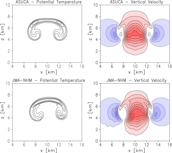
b. Rising thermal simulation

Numerical simulation for a rising thermal in a uniform horizontal flow in a two-dimensional adiabatic atmosphere, based on Wicker and Skamarock (1998), was performed to evaluate basic performance for idealized convection and advection. The grid spacing is 125 m in both the x- and z-directions, and the computational domain is 20-km wide and 10-km deep. The initial thermal (diameter: 4 km) is placed at a height of 2 km, with a potential temperature of 2 K higher than the surrounding environment and neutral stratification. The test imposes a uniform horizontal flow of 20 m s⁻¹ and integrated for 1000 s so that the thermal is laterally advected in a horizontally periodic domain and should be located in the center of the horizontal domain. A time-step interval of 2 s is used for ASUCA, while a 1-s time interval is used for the JMA-NHM because serious deterioration in simulation is produced with a 2-s interval.

Figure 7 shows the results for ASUCA and the JMA-NHM. The potential temperature and vertical velocity fields with ASUCA are symmetrical, whereas the potential temperature field with the JMA-NHM is much less symmetrical and the vertical velocity field is distorted and dispersive. The asymmetric result produced by JMA-NHM is mainly due to its fourth-order advection and leapfrog time integration scheme, as shown by Wicker and Skamarock (1998). The normalized L2 norm of the error in the vertical velocity, using the results from each model simulation with no horizontal flow as the benchmark, are 0.189 for ASUCA and 0.236 for JMA-NHM, respectively.

Fig. 7.

Results for rising thermal in a uniform horizontal flow testing simulated using (top) ASUCA and (bottom) the JMA-NHM. The panels on the left and right show potential temperature (contour interval 0.25 K) and vertical velocity (contour interval 1.5 m s⁻¹), respectively.

6.2 Performance as an operational NWP

This section compares the performance of the ASUCA-LFM (the 2-km-resolution operational regional model) to that of the NHM-LFM (Aranami et al. 2015).

A simulation involving Karman vortex streets, which often form downwind of islands during the cold-air outbreaks in winter, is presented here as an example of favorable representation using ASUCA dynamics. In Fig. 8, the ASUCA-LFM reproduces the phenomenon better than the NHM-LFM. The JMA-NHM with numerical diffusion coefficients weaker than those of operational configuration could reproduce the Karman vortexes streets. However, these weakened values frequently cause computational instability.

Fig. 8.

(a) Visible satellite imagery from 0530 UTC on 9 January 2015. Cloud fraction at low level simulated using (b) ASUCA-LFM and (c) NHM-LFM with a 5.5-hour lead time and an initial time of 0000 UTC on 9 January 2015.

In regional models, the predicted synoptic-scale pressure field should be consistent with that prescribed as the lateral boundary condition. Figure 9 shows differences in sea level pressure forecasts between the LFM and the external model (MSM) providing the boundary condition for 1200 UTC on 25 December 2012. The ASUCA-LFM (left) follows MSM prediction at the synoptic-scale, while the local patterns differ due to differences in their prediction properties. However, the synoptic-scale pressure field determined from the NHM-LFM (right) deviates from the prediction of the MSM. This superior consistency mainly comes from improved total mass conservation in the ASUCA-LFM. The lateral boundaries control the net mass flux of the model domain and consequently control the synoptic-scale pressure field. ASUCA explicitly calculates mass inflow and outflow because density is directly integrated as a prognostic variable. Accordingly, mass change across the entire domain coincides exactly with the total mass change due to inflow and outflow imposed at the region boundaries, source and sink at the surface, and density change by Rayleigh damping. However, the NHM-LFM, in which pressure is a prognostic variable, does not readily conserve total mass because errors are inevitable in evaluating density from the equation of state.

Fig. 9.

Sea level pressure simulated using (a) ASUCA-LFM and (b) NHM-LFM. Black and red contours indicate sea level pressure [hPa] in the LFM with a 9-hour lead time and an initial time of 0300 UTC on 25 December 2012 and the MSM with a 12-hour lead time and an initial time of 0000 UTC on 25 December 2012, respectively. Shading represents sea level pressure differences between the LFM and the MSM.

The ASUCA-LFM also achieved higher NWP performance, including quantitative precipitation forecast (QPF) accuracy, than NHM-LFM (Fig. 10). Note that the QPF change is attributed to the updates of physical process schemes and the dynamical core itself. As it was also confirmed that ASUCA-LFM had better performance in terms of consistency with ground-based and radiosonde observations, ASUCA replaced JMA-NHM as the LFM in 2015 and the MSM in 2017 subsequently.

Fig. 10.

The threat score (TS; left) and the bias score (BI; right) for 1-hour precipitation accumulation with ASUCA-LFM(red) and NHM-LFM (blue), for a threshold of 1 mm h⁻¹. The forecasts are verified against the Radar/Rainguage-Analyzed Precipitation, which is operationally produced by JMA, for the summer season in 2012. TS measures the fraction of observed and/or forecast events that were correctly forecasted, and the accuracy of forecasts is higher as TS approaches to the maximum value of unity. BI measures the frequency correspondence between forecast and observation events. If BI is larger (smaller) than unity, the frequency of events is overestimated (underestimated).

7. Future plans

As described in Section 1, the development of the new nonhydrostatic numerical model ASUCA was begun in 2007. The model is designed to ensure accuracy for NWP model; maintainability of components, including physical processes; and the data assimilation system and code structure suitable for future supercomputer architectures toward the establishment of a long-term operational forecasting infrastructure with a new-generation NWP model. ASUCA replaced the previous regional NWP model JMA-NHM (Saito et al. 2006) in 2015 as the LFM with a 2-km resolution and in 2017 as the MSM with a 5-km resolution. The ASUCA-based Mesoscale Ensemble Prediction System (Ono et al. 2021) has been in operation since 2019 and the ASUCA-based 4D-Var system (Ikuta et al. 2021), which is an outcome of relational developments, has been used to provide initial MSM fields since 2020. We close this paper with some ongoing development of ASUCA.

Increases in computational power in the future enable us to operate a regional NWP with higher model resolution and a wider forecast region, which could contribute to improving forecasts of severe weather. However, this may also create new issues to be addressed in the improvement of high-resolution model accuracy.

While numerical models start to partly resolve cumulus convection with increased resolution, unresolved motions remain to be parameterized due to the incompleteness of the motions resolved in the model. As assumptions made in conventional parameterization schemes are also often violated in such a regime, new parameterization schemes suitable for partially unresolved processes are required. This is known as the gray zone problem, which has recently drawn attention in the fields of research on cumulus convection (e.g., Arakawa and Wu 2013) and boundary layer turbulence (Honnert et al. 2020). It should be emphasized that the improvement of dynamical processes is even more important than ever in the gray zone as the resolved part, which is represented by dynamical processes, increases at higher resolution.

The utilization of Koren's flux limiter enables the elimination of an explicit numerical filter and only advection scheme involves diffusion, which highly depends on wind speed and direction (i.e., acting only in the windward direction). This results in overly frequent prediction of intense vertical velocity because diffusion relating to horizontal advection is relatively small in such situations. Accordingly, parameterization of horizontal diffusion with physical consideration may be necessary.

Some recent convection schemes (e.g., Kuell et al. 2007; Malardel and Bechtold 2019) relax the conventional assumption that the change in density by convection is negligible (i.e., environmental subsidence cancels the convective mass fluxes). The coupling of such physics schemes with the current dynamical core is a significant challenge because terms evaluated by those schemes relate to sound waves and their implementation may require the modification of the HE-VI scheme.

A numerical model with higher spatial resolution can also resolve smaller scales of topography, whose favorable representation helps improve the model performance (Kanehama et al. 2019; Sandu et al. 2019). For instance, local circulation and precipitation processes derived from the topography can be more accurate. However, finer topographical representations incorporating steep slopes can significantly distort the shape of the control volume and affect numerical stability because the vertical axis in the terrain-following coordinate is restricted to the direction of gravity in the current configuration.

Steeper terrain can also cause significant pressure gradient force errors. In slope-containing grids, the evaluation of horizontal pressure gradient force requires consideration of the vertical pressure gradient in generalized coordinates as per Eqs.(10) and (11). As the centered difference is used for the vertical pressure gradient, pressure is linearly interpolated using surrounding pressure values. Linear vertical interpolation of pressure creates larger discretization errors for steeper slopes because pressure changes with height are almost exponential. Modification of pressure gradient force computation via the interpolation of pressure to a constant height for adjacent columns (e.g., Klemp 2011) may reduce such errors. However, this requires further consideration in future work.

The currently operational nonhydrostatic model ASUCA has improved NWP accuracy for heavy rain and typhoons and contributing to a better understanding of extreme weather conditions around Japan and Asia. Ongoing development of the model is expected to improve NWP accuracy even more.

Data Availability Statement

Some of the datasets and program codes used in this study are not publicly available due to the management policy of the Japan Meteorological Agency, but may be available from the relevant authors for reasonable usage upon request. All rights remain with JMA.

Acknowledgments

We gratefully acknowledge all the colleagues developing ASUCA. We are also grateful to Dr. Nigel Wood and one anonymous reviewer who gave their constructive comments to help us improve quality of our manuscript.

Appendix A: List of symbols

Symbols used in this paper are listed below in alphabetical order. The subscript α refers to dry air, water vapor, cloud water, cloud ice, rain, snow, and graupel for d, v, c, i, r, s, and g, respectively. Cartesian coordinates and generalized coordinates are referred to as (x, y, z) and (ξ, η, ζ), respectively.

Appendix B: Map projection and vertical coordinates in the operational models

The details of map projection and the vertical coordinates employed in the LFM and MSM, which are operational regional NWP with 2-km and 5-km resolutions, respectively, are presented here.

ASUCA employs the Lambert conformal map projection. The map factors m₁ and m₂ (for the x- and y-directions) here are given by   

  

where ϕ is the latitude, and ϕ₁ = 30° and ϕ₂ = 60° are used as the standard parallels in the operational models.

The hybrid terrain-following vertical coordinate (Ishida 2007) is adopted to reduce the influences of topography with height. Since the horizontal pressure gradient term and the horizontal advection term are split into horizontal and vertical derivatives with non-flat coordinates and the vertical grid spacing of NWP models is generally larger in the upper atmosphere, the reduction of errors associated with related difference calculation is advantageous. The vertical coordinate ζ is transformed using   

where z is height above sea level and z_s is ground height. The function h (ζ) is given by   

where z_T is the model top. z_c and n are the parameters characterizing the influence of terrain; z_c is the height at which the center of the transition, between the terrain-following coordinate and the flat coordinate, is located; and n determines the varying rate of the transition. z_c = 7000 m and n = 3 are employed in the LFM and MSM. Figure B1 shows the model levels over idealized mountain in the hybrid terrain-following coordinate in contrast to the basic terrain-following coordinate (Gal-Chen and Somerville 1975). The hybrid terrain-following coordinate is identical to the terrain-following and flat coordinates at z = z_s and z = z_T, respectively, and the two coordinates are smoothly connected.

Fig. B1.

The model vertical half-levels in the hybrid terrain-following (left) and classical terrainfollowing (right) coordinates over idealized mountain with the maximum height of 2000 m. Every five layers are highlighted with thick lines. The LFM configuration is used for the coordinate parameters and the model top.

Appendix C: CFL condition for the advection with the Koren flux limiter and RK3 scheme

The one-dimensional advection equation with a uniform velocity u (> 0) is considered as follows:   

The spatial direction is discretized with the grid spacing Δx = 2π/N (N : the number of grid cells). We assume the following solution in Eq. (62):   

The advection term is approximated by the first- or third-order upwind difference in the Koren flux limiter. The spatial derivative at the j-th grid using Eq. (63) is represented as   

for the first-order upwind difference. Substituting Eq. (64) into Eq. (62) yields   

In the third-order Runge–Kutta time integration, Eq. (65) is stable if   

is satisfied for 0 ≤ k Δ x ≤ π. Here, the superscript n denotes the n-th timestep and C₁ = uΔt/Δx is the Courant number. Solving Eq. (66) numerically, we can obtain the CFL condition C₁ ≤ 1.25 for the first-order upwind difference.

The spatial derivative for the third-order upwind difference is written as   

The CFL condition C₁ ≤ 1.61 for the third-order upwind difference can be obtained by the similar procedure. This value coincides with that by Wicker and Skamarock (2002). Because the critical value of C₁ for the first order is smaller than that for the third order, C₁ ≤ 1.25 should be chosen as the CFL condition for the Koren flux limiter.

References

•  Arakawa,  A., and  V. R.  Lamb, 1977: Computational design of the basic dynamical processes of the UCLA general circulation model. General Circulation Models of the Atmosphere. Methods in Computational Physics: Advances in Research and Applications, Vol. 17, Elsevier, 173-265.
•  Arakawa,  A., and  C.-M.  Wu, 2013: A unified representation of deep moist convection in numerical modeling of the atmosphere. Part I. J. Atmos. Sci., 70, 1977-1992.
•  Aranami,  K., and  J.  Ishida, 2004: Implementation of two dimensional decomposition for JMA non-hydrostatic model. CAS/JSC WGNE Res. Activ. Atmos. Oceanic Modell., 34, 0301-0302.
•  Aranami,  K.,  T.  Hara,  Y.  Ikuta,  K.  Kawano,  K.  Matsubayashi,  H.  Kusabiraki,  T.  Ito,  T.  Egawa,  K.  Yamashita,  Y.  Ota,  Y.  Ishikawa,  T.  Fujita, and  J.  Ishida, 2015: A new operational regional model for convection-permitting numerical weather prediction at JMA. CAS/JSC WGNE Res. Activ. Atmos. Oceanic Modell., 45, 0505-0506.
•  Beljaars,  A. C. M., and  A. A. M.  Holtslag, 1991: Flux parameterization over land surfaces for atmospheric models. J. Appl. Meteor., 30, 327-341.
•  Cats,  G.,  V. T.  Vu, and  L.  Wolters, 2008: Overlapping communications with calculations. HIRLAM Newslett., 54, 189-201.
•  Coakley,  J. A., Jr.,  R. D.  Cess, and  F. B.  Yurevich, 1983: The effect of tropospheric aerosols on the Earth's radiation budget: A parameterization for climate models. J. Atmos. Sci., 40, 116-138.
•  Dubal,  M., N.,  N.  Wood, and  A.  Staniforth, 2004: Analysis of parallel versus sequential splittings for time-stepping physical parameterizations. Mon. Wea. Rev., 132, 121-132.
•  Durran,  D. R., 2010: Numerical Methods for Fluid Dynamics: With Applications to Geophysics. 2nd Edition. Texts in Applied Mathematics, Vol. 32, Springer New York, 516 pp.
•  Gal-Chen,  T., and  R. C. J.  Somerville, 1975: On the use of a coordinate transformation for the solution of the Navier-Stokes equations. J. Comp. Phys., 17, 209-228.
•  Gassmann,  A., and  H.-J.  Herzog, 2007: A consistent time-split numerical scheme applied to the nonhydrostatic compressible equations. Mon. Wea. Rev., 135, 20-36.
•  Godunov,  S. K., 1959: A difference method for numerical calculation of discontinuous solutions of the equations of hydrodynamics. Mat. Sb. (N.S.), 47, 271-306 (in Russian).
•  Gryanik,  V. M.,  C.  Lüpkes,  A.  Grachev, and  D.  Sidorenko, 2020: New modified and extended stability functions for the stable boundary layer based on SHEBA and parametrizations of bulk transfer coefficients for climate models. J. Atmos. Sci., 77, 2687-2716.
•  Gunn,  R., and  G. D.  Kinzer, 1949: The terminal velocity of fall for water droplets in stagnant air. J. Meteor., 6, 243-248.
•  Hara,  T.,  K.  Kawano,  K.  Aranami,  Y.  Kitamura,  M.  Sakamoto,  H.  Kusabiraki,  C.  Muroi, and  J.  Ishida, 2012: Development of the physics library and its application to ASUCA. CAS/JSC WGNE Res. Activ. Atmos. Oceanic Modell., 42, 0505-0506.
•  Honnert,  R.,  G. A.  Efstathiou,  R. J.  Beare,  J.  Ito,  A.  Lock,  R.  Neggers,  R. S.  Plant,  H. H.  Shin,  L.  Tomassini, and  B.  Zhou, 2020: The atmospheric boundary layer and the “gray zone” of turbulence: A critical review. J. Geophys. Res.: Atmos., 125, e2019JD030317, doi: 10.1029/2019JD030317.
•  Ikawa,  M., and  K.  Saito, 1991: Description of a nonhydrostatic model developed at the Forecast Research Department of the MRI. Tech. Rep. Meteor. Res. Inst., No. 28, 238 pp (with Japanese abstract).
•  Ikuta,  Y.,  T.  Fujita,  Y.  Ota, and  Y.  Honda, 2021: Variational data assimilation system for operational regional models at Japan Meteorological Agency. J. Meteor. Soc. Japan, 99, 1563-1592.
•  Ishida,  J., 2007: Development of a hybrid terrain-following vertical coordinate for JMA Non-hydrostatic Model. CAS/JSC WGNE Res. Activ. Atmos. Oceanic Modell., 37, 0309-0310.
•  Ishida,  J.,  C.  Muroi,  K.  Kawano, and  Y.  Kitamura, 2010: Development of a new nonhydrostatic model “ASUCA” at JMA. CAS/JSC WGNE Res. Activ. Atmos. Oceanic Modell., 40, 0511-0512.
• Japan Meteorological Agency, 2014: ASUCA: Next generation non-hydrostatic model. Separate volume of annual report of Numerical Prediction Division, No. 60, 156 pp (in Japanese). [Available at https://www.jma.go.jp/jma/kishou/books/nwpreport/60/No60_all.pdf.]
• Japan Meteorological Agency, 2019a: Computer system. Outline of the operational numerical weather prediction at the Japan Meteorological Agency. 1-8. [Available at https://www.jma.go.jp/jma/jma-eng/jmacenter/nwp/outline2019-nwp/index.htm.]
• Japan Meteorological Agency, 2019b: Numerical weather prediction models. Outline of the operational numerical weather prediction at the Japan Meteorological Agency. 47-138. [Available at https://www.jma.go.jp/jma/jma-eng/jma-center/nwp/outline2019-nwp/index.htm.]
•  Joseph,  J. H.,  W. J.  Wiscombe, and  J. A.  Weinman, 1976: The delta-Eddington approximation for radiative flux transfer. J. Atmos. Sci., 33, 2452-2459.
•  Kain,  J. S., 2004: The Kain-Fritsch convective parameterization: An update. J. Appl. Meteor., 43, 170-181.
•  Kain,  J. S., and  J. M.  Fritsch, 1990: A one-dimensional entraining/detraining plume model and its application in convective parameterization. J. Atmos. Sci., 47, 2784-2802.
•  Kanehama,  T.,  I.  Sandu,  A.  Beljaars,  A.  van Niekerk, and  F.  Lott, 2019: Which orographic scales matter most for medium-range forecast skill in the Northern Hemisphere winter? J. Adv. Model. Earth Syst., 11, 3893-3910.
•  Klemp,  J. B., 2011: A terrain-following coordinate with smoothed coordinate surfaces. Mon. Wea. Rev., 139, 2163-2169.
•  Klemp,  J. B.,  W. C.  Skamarock, and  J.  Dudhia, 2007: Conservative split-explicit time integration methods for the compressible nonhydrostatic equations. Mon. Wea. Rev., 135, 2897-2913.
•  Koren,  B., 1993: A robust upwind discretization method for advection, diffusion and source terms. Numerical Methods for Advection-Diffusion Problems.  Vreugdenhil,  C. B.,  Koren,  B. (eds.), Vieweg, 117-138.
•  Kuell,  V.,  A.  Gassmann, and  A.  Bott, 2007: Towards a new hybrid cumulus parametrization scheme for use in non-hydrostatic weather prediction models. Quart. J. Roy. Meteor. Soc., 133, 479-490.
•  Lin,  Y.-L.,  R. D.  Farley, and  H. D.  Orville, 1983: Bulk parameterization of the snow field in a cloud model. J. Appl. Meteor. Climatol., 22, 1065-1092.
•  Lorenz,  E. N., 1960: Energy and numerical weather prediction. Tellus, 12, 364-373.
•  Malardel,  S., and  P.  Bechtold, 2019: The coupling of deep convection with the resolved flow via the divergence of mass flux in the IFS. Quart. J. Roy. Meteor. Soc., 145, 1832-1845.
•  Moncrieff,  M. W.,  S. K.  Krueger,  D.  Gregory,  J.-L.  Redelsperger, and  W.-K.,  Tao, 1997: GEWEX Cloud System Study (GCSS) working group 4: Precipitating convective cloud systems. Bull. Amer. Meteor. Soc., 78, 831-846.
•  Nakanishi,  M., and  H.  Niino, 2009: Development of an improved turbulence closure model for the atmospheric boundary layer. J. Meteor. Soc. Japan, 87, 895-912.
•  Noilhan,  J., and  S.  Planton, 1989: A simple parameterization of land surface processes for meteorological models. Mon. Wea. Rev., 117, 536-549.
•  Ono,  K.,  M.  Kunii, and  Y.  Honda, 2021: The regional model-based Mesoscale Ensemble Prediction System, MEPS, at the Japan Meteorological Agency. Quart. J. Roy. Meteor. Soc., 147, 465-484.
•  Saito,  K.,  T.  Kato,  H.  Eito, and  C.  Muroi, 2001: Documentation of the Meteorological Research Institute/Numerical Prediction Division Unified Nonhydrostatic Model. Tech. Rep. Meteor. Res. Inst, NO. 42, 133 pp.
•  Saito,  K.,  T.  Fujita,  Y.  Yamada,  J.  Ishida,  Y.  Kumagai,  K.  Aranami,  S.  Ohmori,  R.  Nagasawa,  S.  Kumagai,  C.  Muroi,  T.  Kato,  H.  Eito, and  Y.  Yamazaki, 2006: The operational JMA nonhydrostatic mesoscale model. Mon. Wea. Rev., 134, 1266-1298.
•  Samukawa,  H., 2001: A parallel tridiagonal solver based on ETC ordering. IPSJ J., 42, 779-787 (in Japanese).
•  Sandu,  I.,  A.  van Niekerk,  T. G.  Shepherd,  S. B.  Vosper,  A.  Zadra,  J.  Bacmeister,  A.  Beljaars,  A. R.  Brown,  A.  Dörnbrack,  N.  McFarlane,  F.  Pithan, and  G.  Svensson, 2019: Impacts of orography on large-scale atmospheric circulation. npj Climate Atmos. Sci., 2, 10, doi: 10.1038/s41612-019-0065-9.
•  Skamarock,  W. C., and  J. B.  Klemp, 1992: The stability of time-split numerical methods for the hydrostatic and the nonhydrostatic elastic equations. Mon. Wea. Rev., 120, 2109-2127.
•  Skamarock,  W. C., and  J. B.  Klemp, 1994: Efficiency and accuracy of the Klemp-Wilhelmson time-splitting technique. Mon. Wea. Rev., 122, 2623-2630.
•  Skamarock,  W. C.,  J.  Doyle,  P.  Clark, and  N.  Wood, 2004: A standard test set for nonhydrostatic dynamical cores of NWP models. Proceeding of 16th Conference on Numerical Weather Prediction, Seattle WA, USA, P2.17. [Available at https://ams.confex.com/ams/84Annual/techprogram/paper_72056.htm.]
•  Straka,  J. M.,  R. B.  Wilhelmson,  L. J.  Wicker,  J. R.  Anderson, and  K. K.  Droegemeier, 1993: Numerical solutions of a non-linear density current: A benchmark solution and comparisons. Int. J. Numer. Methods Fluids, 17, 1-22.
•  Sweby,  P. K., 1984: High resolution schemes using flux limiters for hyperbolic conservation laws. SIAM J. Numer. Anal., 21, 995-1011.
•  Wicker,  L. J., and  W. C.  Skamarock, 1998: A time-splitting scheme for the elastic equations incorporating second-order Runge-Kutta time differencing. Mon. Wea. Rev., 126, 1992-1999.
•  Wicker,  L. J., and  W. C.  Skamarock, 2002: Time-splitting methods for elastic models using forward time schemes. Mon. Wea. Rev., 130, 2088-2097.
•  Yabu,  S., 2013: Development of longwave radiation scheme with consideration of scattering by clouds in JMA global model. CAS/JSC WGNE Res. Activ. Atmos. Oceanic Modell., 43, 0407-0408.