Abstract
The observation operator (OO) is essential in data assimilation (DA) to derive the model equivalent of observations from the model variables. In the satellite DA, the OO for satellite microwave brightness temperature (BT) is usually based on the radiative transfer model (RTM) with a bias correction procedure. To explore the possibility to obtain OO without using physically based RTM, this study applied machine learning (ML) as OO (MLOO) to assimilate BT from Advanced Microwave Sounding Unit-A (AMSU-A) channels 6 and 7 over oceans and channel 8 over both land and oceans under clear-sky conditions. We used a reference system, consisting of the nonhydrostatic icosahedral atmospheric model (NICAM) and the local ensemble transform Kalman filter (LETKF). The radiative transfer for TOVS (RTTOV) was implemented in the system as OO, combined with a separate bias correction procedure (RTTOV-OO). The DA experiment was performed for 1 month to assimilate conventional observations and BT using the reference system. Model forecasts from the experiment were paired with observations for training the ML models to obtain ML-OO. In addition, three DA experiments were conducted, which revealed that DA of the conventional observations and BT using ML-OO was slightly inferior, compared to that of RTTOV-OO, but it was better than the assimilation based on only conventional observations. Moreover, ML-OO treated bias internally, thereby simplifying the overall system framework. The proposed ML-OO has limitations due to (1) the inability to treat bias realistically when a significant change is present in the satellite characteristics, (2) inapplicability for many channels, (3) deteriorated performance, compared with that of RTTOV-OO with respect to accuracy and computational speed, and (4) physically based RTM is still used to train the ML-OO. Future studies can alleviate these drawbacks, thereby improving the proposed ML-OO.
1. Introduction
Data assimilation (DA) is a combination of model simulations and observations. DA provides an optimal estimate of the initial condition, thereby improving the forecast. Because satellite observations provide dominant observational information for global numerical weather predictions (NWP) (Eyre et al. 2020), assimilating them is important. In this context, the Advanced Microwave Sounding Unit-A (AMSU-A) is a multichannel microwave radiometer, which is sensitive to the temperature profile of the atmosphere. It has been already used for improving NWP performance [e.g., Miyoshi et al. 2010; Terasaki and Miyoshi 2017 (hereafter simply “TM17”)]. For atmospheric DA, the model space and the observation space are generally different because the locations of the observations do not ideally coincide with the model grid points, and the observed variables may not be the same as the model variables. Due to this, to compare the model state and observations, an observation operator (OO) (e.g., a forward model) is required. When satellite radiances are used as observations, the OO has two primary purposes. First, it performs a horizontal interpolation of the model variables at the model grids to the observation locations. Second, at each observation location, the simulated (synthetic) radiance is calculated using a vertical profile of the model variables (Kalnay 2002, p. 161). In the present study, we elucidated only the second aspect, which requires knowledge about the relationships between model variables and satellite radiances. To fulfill this, there are two approaches: physically based radiative transfer models (RTMs; RTM-OO) and machine learning (ML) models (ML-OO).
From the RTM-OO perspective, the line-by-line (LBL) RTM is an accurate and flexible RTM, applicable over a full spectral range. Such ability lays the foundation for several radiative transfer applications (Alvarado et al. 2013). As the calculation of the RTM needs to be fast for DA, it is generally not recommended to use LBL RTM for RTM-OO. Therefore, faster RTMs have been developed. For instance, in the radiative transfer for TOVS (RTTOV) (Saunders et al. 2018), the layer optical depth for specific gas and channel is parameterized in terms of layer mean atmospheric variables (Saunders et al. 2018; Hocking 2019). To obtain the regression coefficients of these predictors, layer-to-space transmittances at high spectral resolutions computed from LBL RTMs using a variety of atmospheric profiles have been used. Notably, fast RTMs such as RTTOV are the most widely used OOs for satellite radiance DA. The biases between the model equivalent of observations from the RTM and the actual satellite observations can emerge due to various effects, including the calibration problem of the instrument, the temporal change of instrument characteristics, the preprocessing of the data, the RTM inaccuracies, and the bias in the model field (Derber 1998; Dee 2004; Harris and Kelly 2001). A bias correction procedure is required for two common types of biases: scan bias and airmass bias (Dee 2004; Harris and Kelly 2001). The former is related to the satellite scan position and latitude, and the latter is related to the state of the atmosphere (Harris and Kelly 2001). Note that some NWP centers use only the scan positions for scan bias correction. Scan bias can be estimated offline (Harris and Kelly 2001) or online (TM17). The airmass bias can be estimated offline (Harris and Kelly 2001). It can also be estimated online adaptively in the variational DA using the variational bias correction (VarBC) method (Derber 1998; Dee 2004). Furthermore, an equivalent method in ensemble DA has been previously proposed (Miyoshi et al. 2010; TM17).
From the ML-OO perspective, MLs are efficient for identifying complex statistical relationships within the data. The application of artificial intelligence and ML in Earth and atmospheric studies has become increasingly popular in research, whereas a review of such applications can be found in Boukabara et al. (2021). ML can be used to reduce the high computational cost in applications that involve complicated physical processes. For instance, ML can be used to emulate and accelerate parametrization schemes in the NWP (Chantry et al. 2021; Pal et al. 2019; Krasnopolsky et al. 2008). Likewise, the ML method can be applied to build an ML-OO. In general, there are primarily two ways to train an ML-OO.
Firstly, one can use the input and output data from the RTM. The development of ML-OO using the RTM requires various input variables, covering the full physical parameter space with sufficient resolution. Such inputs are provided to the RTM to generate the corresponding synthetic radiances. The input variables and output radiances are paired to train an ML model to obtain the ML-OO. If the original RTM is computationally expensive, ML-OO can generally reduce the computational cost while retaining sufficient accuracy. For instance, a look-up table can be generated by the ML emulator to be further used for retrieval purposes (Rivera et al. 2015). In Scheck (2021), slow RTM for visible satellite images was emulated using a neural network (NN).
Secondly, it is possible to develop the ML-OO without the use of RTM. Compared to the method using RTM, such an approach relies on satellite-observed radiance data instead of synthetic radiance data from the RTM. Being combined with the model state, satellite radiance can be used to train the ML model. To represent the actual relationship between the model state and the satellite radiance, the model state used for training the ML-OO must be good enough. To this end, we suggest that analyses or short-term forecasts after analyses from DA and reanalysis data can be used. Kwon et al. (2019) have previously used atmospheric reanalysis data to provide forcing for a land surface model to generate synthetic snow depth. Then, synthetic snow depth and observed radiance were utilized to train a support vector machine model. They showed that ML-OO is computationally more efficient than RTM. To the best of our knowledge, the analyses or short-term forecasts from DA were never utilized to combine with the satellite-observed radiance to train an ML model.
Our goal is to build an ML-OO without using the RTM. However, this study is only the first step since we still used RTM to assimilate the satellite radiance to generate better short-term forecasts. As mentioned earlier, the bias between synthetic radiance and satellite-observed radiance should be addressed. Zhou and Grassotti (2020) used ML to address the radiometric bias to improve the satellite retrievals. Rodríguez-Fernández et al. (2019) have previously trained the ML model using the Soil Moisture and Ocean Salinity brightness temperature (BT) from observations as the input and soil moisture (SM) from the model as the output. They found no global bias between the retrieved SM predicted from the ML and the modeled SM. Similarly, if ML-OO for satellite radiance is built using the model state and the observed radiance, the bias between the simulated radiance from ML-OO and the observed radiance would be assumingly low. As one of the objectives of the study, we evaluate this surmise by our analysis. Moreover, we compare ML-OO with the RTM-OO. Finally, we discuss how our preliminary study can be extended to broader applications.
The remainder of this paper is organized as follows. Section 2 describes the materials and methods. Sections 3 and 4 present the experimental setup and results, respectively. Finally, Sections 5 and 6 give a discussion and summary, respectively.
2. Materials and methods
2.1 DA system
In the current study, we used the nonhydrostatic icosahedral atmospheric model (NICAM) (Satoh et al. 2014) and the local ensemble transform Kalman filter (LETKF) (Hunt et al. 2007) to conduct DA experiments. The configuration of the system (NICAM-LETKF) mostly followed that of the TM17. In the present study, only a few important aspects of the system related to this study are presented. The horizontal resolution of the NICAM was 112 km. There were 78 vertical levels (38 levels in TM17) up to the height of ∼ 50 km. The NICAM-LETKF has an OO for assimilating the satellite radiance. The OO horizontally interpolates model variables in the first guess from the model grids to the observation locations. These variables include pressure, temperature, specific humidity, surface pressure, 2-m temperature, surface (skin) temperature, 2-m specific humidity, and 10-m zonal/meridional winds. After the interpolation, at each observation location, the interpolated model variables combined with other variables were utilized in RTTOV (version 12.2) to calculate the model equivalent of the BT. A complete list of the variables required by the RTTOV can be found in Hocking (2019). The NICAM-LETKF system uses an online bias correction method to correct scan bias and airmass bias (TM17). The biases were estimated adaptively during the DA and subtracted from the observed BT before the analysis. The input variables (predictors) for the airmass bias included the integrated weighted lapse rate (IWLR) at two layers, namely, 1000–200 hPa and 200–50 hPa, the surface temperature, and the inverse of cosine of satellite zenith angle. For brevity, we use the RTTOV-OO to indicate the OO based on RTTOV combined with an online bias correction method.
The NICAM-LETKF system contained 64 ensemble members. The relaxation to prior spread method was applied for covariance inflation (Whitaker and Hamill 2012; Kotsuki et al. 2017). Covariance localization based on the Gaussian function was applied with a standard deviation σ = 250 km in the horizontal and 0.4 in the vertical natural-log-pressure coordinate, but the localization function was replaced by zero beyond  . Note that vertical localization was not used for AMSU-A BT. Its impact on performance will be investigated in future studies.
2.2 Observation data
Observations were assimilated every 6 h (Fig. 1a). At each analysis time point, the observations within the ±3 h time window were assimilated. Overall, there were seven observation files (time slots) in an analysis time window. One file in each time slot contained observations ±30 min. After finishing an analysis, we forecasted 9 h so that there were observations within the ±3 h time window at the next analysis time. This process was continued until the end of the experimental period.

The observations included the NCEP ADP Global Upper Air and Surface Weather Observations dataset (NCEP PREPBUFR). This dataset includes records from radiosondes, wind profilers, aircraft, land surface observations, marine observations, atmospheric motion vectors, and sea surface winds from satellite scatterometers. The satellite radiance data were represented by BT obtained from the AMSU-A instruments onboard the NOAA-15, NOAA-18, NOAA-19, METOP-A, and METOP-B satellites. Note that in this study, the term “conventional observations” indicates the observations from the NCEP PREPBUFR dataset. As our model was vertically constrained by the 50 km height in this study, we assimilated only the channel numbers 6, 7, and 8. The channels 9 and beyond, which are sensitive to the stratosphere and mesosphere, were not assimilated due to this reason. Moreover, the lower channels were not assimilated due to their sensitivity to the lower troposphere and the Earth's surface, where the quality control in this study was rather simplistic to handle the data (TM17). Not all three channels were assimilated for some satellites (Table 1). The standard deviation of the observation error used for DA was set at 0.3 K for all the used channels.

Before the DA, the observations were preprocessed, where data thinning, quality control, and gross error checks were applied to the observations. The observation errors in DA include measurement and representation errors (Janjić et al. 2018). The observation errors are correlated with respect to space and time. Particularly, for satellite radiances, correlated errors may be present between channels. However, it is challenging to identify and implement a full observation error-covariance matrix for such data. Therefore, spatial thinning was implemented in this study to reduce potential spatial correlations. For thinning of the AMSU-A observations, we selected the nearest observations from every grid point of the uniform virtual horizontal grids with the 250-km resolution by following the JMA's setting from Okamoto et al. (2005). Note that a thorough examination of the thinning distance effects is beyond the scope of this study. Furthermore, the quality control for assimilating AMSU-A was applied after thinning. The observations from channels 6 and 7 over the land were completely filtered out. Over the oceans, observations from these two channels were filtered out at the liquid water path (LWP) > 0.12 kg kg−1 and 0.15 kg kg−1, respectively. The LWP was calculated using channels 1 and 2 from AMSU-A (Grody et al. 2001). LWP was utilized to remove cloud- and rain-contaminated observations by following the method of Bormann et al. (2012). Channel 8 was assimilated without any quality control because the peak height of the weighting function is higher, which implies that this channel is less affected by clouds and rain. Finally, we performed a gross error check to remove the data with a large observation-minus-first-guess departure. Specifically, when the departure was greater than three times the standard deviation of the observation error, the data were filtered out. To train the ML model, the same quality control was applied to the AMSU-A observations. However, data thinning of AMSU-A observations was not applied because more data were required to train the ML model. As shown in Fig. 1b, after the quality control, all the data over land from channels 6 and 7 were excluded, whereas there were data over land and oceans from channel 8.
2.3 ML method
As discussed in the Introduction section, the OO interpolates and converts the model variables into the model equivalent of the observation. To build a good OO, we should ideally use the values of the model variables and observed variables that are close to the true state of the atmosphere. In this context, DA is necessary to obtain such model variable values. On this basis, we opted to use the model forecasts after assimilating conventional observations and AMSU-A (using RTTOV-OO) as the input data for building the ML model. At every analysis time slot (00 UTC, 06 UTC, 12 UTC, 18 UTC), a 9-h forecast was performed, thereby yielding the hourly forecast data from 3 h to 9 h after the analysis. Instead of using the forecasts at all 7 h as the input to train the ML model, we used only the forecasts from 3 h to 6 h after each time slot of the analysis. Fundamentally, they were closer to the analysis, while the satellites also had global coverage in this time window. Note that the experiments that produced model forecasts from the NICAM-LETKF will be explained in Section 3.
For each atmospheric column, we would like to use ML-OO to predict BT according to the related model variables in the same column. On this basis, the development of the ML model implied that the input data (model variables) and output data (BT) in the same row of the dataset should originate from the same atmospheric column. As observation locations differed from the model grids, we interpolated the model variables at the model grids to the observation locations. Note that most input variables of the ML model were the same as RTTOV-OO (Table 2). For the three-dimensional variables, such as pressure, temperature, and specific humidity, each layer was considered as a feature in the ML model. However, the specific humidity above the NICAM level 40 (∼ 200 hPa height) was constant and almost 0. They were excluded as features because constant inputs do not contribute to the input–output relationship (Krasnopolsky et al. 2008).

Moreover, we added two predictors for the biases to the input variables because our initial idea was to ensure that the ML model can capture biases. The sections below briefly describe how biases had been treated by previous studies and explain how the ML treats biases in this study. In the offline bias correction method (Harris and Kelly 2001; Dee 2004), the bias corrections were precomputed using historical data using the following steps: (1) the scan bias coefficient bscan (θ, Ø) is obtained. It is a function of scan angle θ and latitude Ø. Then, (2) the scan bias is removed from the departures: y − h (xb) − bscan (θ, Ø), where y is the observation, xb is the model background (usually in the vicinity of the radiosonde to ensure accuracy), and h ( ) is the RTM. y − h (xb) − bscan (θ, Ø) is then fit by a linear regression model. The linear regression model is the airmass bias correction term in this case.
where
N is the number of predictors,
pi (
i = 0, ...,
N) are the predictors (state-dependent),
βi (
i = 0, ...,
N) are the coefficients of the predictors, and
ẽ is the residual error. As linear regression always passes the center of the data, the expectation of the residual errors is zero. The coefficients of scan bias and airmass bias are stored in the file and were used in the DA.
Eq. (1) can be changed to:
Therefore, before assimilating an observation y, the scan bias and the airmass bias are removed from the observations to obtain a “bias-corrected” observations y′, which are subsequently assimilated. In the end, because 〈ẽ〉 = 0, there is no bias between the simulated radiance h (xb) and the “bias-orrected” radiance y′.
Furthermore, the constant coefficients of the predictors for the airmass bias correction can be updated adaptively during DA. In VarBC, the coefficients of the predictors are added to the model state to form an augmented vector. The original OO is modified using the airmass bias term. The minimization of the cost function updates the augmented vector and the coefficients of the predictors, as shown by equations 10–14 of Dee (2004). The ensemble-based VarBC in the ensemble DA also updates the coefficients adaptively based on the formulas from VarBC. Note that for VarBC and ensemble-based VarBC, the cost function contains two terms: distance to the background and distance to the observations. Thus, its minimization cannot ensure the minimization of the bias. However, some previous studies, mentioned in the Introduction section, have demonstrated the efficiency of these methods.
Being inspired by the methods above, we argue that ML-OO can also handle the bias. Equation (1) can be rewritten as:
If the observation y on the left-hand side of Eq. (3) and xb, θ, Ø, p on the right-hand side are given, ML can be used to find a function to fit the observations.
where
hml is the ML-OO, and
eml is the residual error of the ML model.
bias = 〈
eml〉.
The ML algorithm minimizes the mean squared error (MSE). The MSE can be decomposed into the variance of the error and the square of the bias (see Appendix A for the derivation).
Because the variance of the error is positive, the square of the bias is smaller than the MSE. If the MSE is reasonably small after the minimization, the absolute value of the bias may be small enough. However, to ensure the performance of the ML-OO, the MSE and bias should be evaluated using the test data after training and before DA. If both MSE and bias are low enough, the ML model can be used as an OO.
In the final step, once the ML-OO is obtained, the DA can be formalized as:
where
xa is the analysis,
xb is the model background, and
K is the optimal weight matrix. Notably, compared with RTTOV-OO, for ML-OO, the original observations can be assimilated directly without subtracting the bias correction terms.
Note that the selection of the predictors in ML-OO was based on the TM17 paper (Table 2). Specifically, in TM17, IWLR, surface temperature, and inverse of the cosine function of the satellite zenith angle were applied as the predictors for airmass bias correction. In the present study, IWLR was not explicitly added because the vertical profiles of pressure and temperature in the input can fundamentally reflect IWLR. Surface temperature and satellite zenith angle are required by the RTM (Saunders et al. 2018). Therefore, they are important for both the radiative transfer process and airmass bias correction. Latitude and satellite scan angle were added to the input variables for the scan bias correction. Note that latitude is also used in RTTOV to calculate the effects of Earth's curvature on the atmospheric path (Hocking 2019). Both latitude and satellite scan angles have been previously applied for scan bias correction by Zhou and Grassotti (2020). They have used ML to correct the bias between the simulated radiances and satellite observations. It is important to note that BT estimates from channels 6, 7, and 8 are not sensitive to the radiation from the surface. However, we included the surface variables in the input of ML-OO. Note that we aim to use similar input variables as RTTOV-OO in TM17 to make the comparison feasible. Moreover, they are the input variables for RTTOV. Finally, these variables are useful for some other channels that are more sensitive to the lower atmosphere. Therefore, we standardized the same set of input variables for all the channels.
Before feeding the data into the ML model, other preprocessing steps were performed. As the specific humidity was skewed toward lower values, we used the log function to transform it to the normal distribution. For the same reason, the pressure was transformed using the log function. The satellite zenith angle was expressed as 1/cos (θ), similar to TM17. Each satellite dataset was separated into a training set (80 %) and a test set (20 %). Finally, the input and output data were standardized to zero mean and unit variance to facilitate the fast convergence of the ML during the training.
Fully connected deep neural networks (DNNs) were used in this study, as shown in Fig. 2. We built different DNNs for each channel and each satellite because the number of collocated observations from the same channel for different satellites is small. Moreover, given the channel-related quality control methods, different channels from the same satellite may have a small number of collocated locations. For example, there were no data from channels 6 and 7 for land, whereas some data were available from channel 8. There were 205 units in the input layer that matched 205 features in the input data. The output layer had only a single unit that corresponded to one channel. The optimizer we used was a gradient descent algorithm known as “Adam”. which is well suited for solving problems that are large with respect to data and/or parameters (Kingma and Ba 2014). We used the rectified linear unit (ReLU) (Glorot et al. 2011) in the hidden layers and linear regression in the output layer. The batch size is the number of training examples used in one iteration. The number is typically selected to be between one and a few hundred (Bengio 2012). For simplicity, it was fixed at 512 in this study. The following hyperparameters were tuned for each DNN model: number of hidden layers, number of units in one hidden layer, and learning rate. For each combination of the above hyperparameters, a DNN was constructed, and it was trained using 80 % of the training set (the training set itself was 80 % of all data) and evaluated using 20 % of the training set (validation set). The validation set was applied for an early stopping to prevent the overfitting of the model. In other words, if the loss function in the validation set starts to increase, overfitting occurs. In the current study, we used the MSE as the loss function. If the MSE of the validation set did not decrease for five consecutive epochs, we stopped the training. During the training, the KerasTuner software (O'Malley et al. 2019) was utilized to automatically conduct a random search for the best combination of hyperparameters for each channel and each satellite. Before the random search, the search spaces for the hyperparameters were set as follows. The numbers of hidden layers were 2, 3, and 4. The unit numbers for each hidden layer were 250, 300, 350, and 400. The learning rates were 10−6 and 10−5.The maximum number of random searches was 25. The combination of hyperparameters that produced the best performance on the validation set was selected for each DNN (Table 3). DNNs were evaluated by comparing the predicted and true values in the test set (Table 3). The coefficient of determination (R2) between the predicted and true values was ∼ 1. The absolute value of the biases was < 0.02 K, whereas the root mean square error (RMSE) was < 0.4 K. As mentioned in the Introduction section, minimizing the MSE using the ML optimization algorithm does not guarantee the minimization of bias. However, the test results revealed low bias. Therefore, the performance of the DNNs was reasonably good, and they were hereafter used as ML-OO in our experiment. A linear regression model was applied to the same dataset for further comparison (Table 3). The RMSEs from the linear regression model were all larger than 1, which was higher than those from the DNN models, whereas the R2 score was also lower. Overall, ML was better than the linear regression approach for solving this problem.

3. Experiments
Several DA experiments were conducted to produce data for training the ML model and for evaluating its performance (Table 4). The experiments were categorized into two groups: experiments for training in 2015 and experiments for testing in 2016. The initial conditions of the ensemble were drawn at the same local time on different days from a single forecast from January to March 2015. Since they differed from the true state of the atmosphere, we needed to spin up the model for 1 month using DA. As discussed in Section 2, a model state close to the true state of the atmosphere is required to build a good ML-OO. Thus, we assimilated the conventional observations as well as AMSU-A BT using RTTOV-OO in Experiments A and B. Note that in this way, we have implicitly used the information from RTM to build the ML-OO. We will discuss how to build ML-OO without using RTM in the Discussion section. Note that an online bias correction method was applied during the experiments. Experiment A was designed to spin up the model. At the end of January 2015, the model state would be close to the true atmosphere. After finishing the spin-up, the DA was continued in February 2015 to generate the model forecasts for training the ML model (Experiment B). After finishing the experiment, the model outputs at the model grids in Experiment B were interpolated to the observation locations. The observations were those without the data thinning and with quality control, as described in Section 2.2 (Fig. 1b). After the interpolation, the (model) first guess at the observation locations and the corresponding AMSU-A BT were paired to train the ML model (Experiment C).

After the ML-OO was built, we evaluated its performance for the same month the following year in 2016. In general, ML can better generalize to new data if it captures more possible combinations and wider ranges of variable values during training. As only 1-month data were used for the training, we also evaluated its performance in the same month of the following year. On 01 January 2016, we used the same initial conditions as in Experiment A. Due to this, we needed to spin up the model using the RTTOV-OO to assimilate the AMSU-A BT and conventional observations (Experiment D). At the end of January 2016, the ensemble members were used for the following DA experiments in February. Experiment E represented the continuation of Experiment D, where we assimilated the conventional observations and AMSU-A BT using RTTOV-OO. In Experiment F, the same observations were assimilated using the ML-OO. Note that no online bias correction was provided for Experiment F because bias correction was included in the ML-OO. The results from Experiments E and F were compared to evaluate the performance of ML-OO compared to RTTOV-OO. Finally, we conducted Experiment G, in which we assimilated only the conventional observations. We compared E against G and F against G to estimate the impact of assimilating the AMSU-A BT using either RTTOV or ML as the OO.
4. Results
The ML models were evaluated in the test experiments. For brevity, we used the annotations CONV-AMSUA-RTTOV, CONV-AMSUA-ML, and CONV to annotate Experiments E, F, and G (Table 4), respectively. Figure 3a illustrates the histogram of the observations minus the model background (OMB) for METOP-B channel 6 from the CONV-AMSUA-ML. The histogram centered at ∼ 0 K. The bias (average of OMB) was estimated to be only 0.002 K, which was the lowest absolute bias among all the channels. Apart from channels 6 and 7 from NOAA-18, all the other channels exhibited similar OMB distributions (figures are omitted) and yielded absolute biases of < 0.1 K (Table 5). However, channels 6 and 7 from NOAA-18 experienced large biases (Fig. 3b) (channel 7 is not shown). The biases from channels 6 and 7 were 0.305 K and 0.259 K, respectively (Table 5). In contrast, the same channels from CONV-AMSUA-RTTOV exhibited much lower biases. For example, it was 0.0461 K for NOAA 18 channel 6 (Fig. 3d). This finding suggests that the bias correction built into the ML-OO might not be effective for these two channels. The horizontal distribution of the OMB demonstrates that the values from METOP-B channel 6 were positive or negative in different regions (Fig. 4a), whereas most of the areas showed positive OMB values from NOAA-18 channel 6 (Fig. 4b). To identify the driver of this pattern, we analyzed the changes of the absolute biases (before the bias correction) from February 2015 to February 2016 from the CONV-AMSUA-RTTOV experiment. The changes were estimated to be 0.17 K and 0.15 K for NOAA-18 channels 6 and 7, respectively. The changes were less than 0.04 K in the other channels. Because the same RTTOV-OO was used for both periods, the changes thereby indicate that the characteristics of observations from NOAA-18 channels 6 and 7 changed significantly from February 2015 to February 2016. As the adaptive bias correction method was applied in CONV-AMSUA-RTTOV, the bias from all channels could be corrected (Figs. 3c, d). However, the training of the ML-OO was based on data from February 2015 and could not treat the bias well in February 2016 with a significant change in satellite characteristics. Previous studies have already shown that the characteristics of satellites can be changed during their operation. For instance, Zou and Wang (2011) have identified bias drifts for some channels of AMSU-A during certain periods. If the change is significant, as shown in our study, the current ML-OO method cannot handle the bias well. Online training by updating pretrained networks using the latest satellite observations can be useful for correcting new biases. However, the frequency to update the ML-OO should be evaluated to balance accuracy and computational cost.


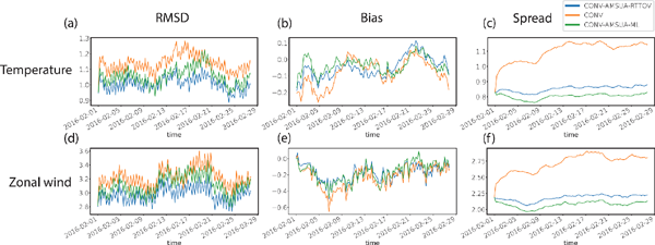
The root mean square difference (RMSD) and bias of temperature and zonal wind from the three experiments were evaluated using the European Centre for Medium-Range Weather Forecasts (ECMWF) reanalysis data (ERA-interim). At 500 hPa, the temperature RMSDs from CONV-AMSUA-ML were generally higher than those from CONV-AMSUA-RTTOV, but lower than those from CONV (Fig. 5a). This indicates that although the performance of ML-OO was slightly worse than that of RTTOV-OO at this level, the assimilation of additional AMSU-A BT by ML-OO improved the forecast, compared with the assimilation of only the conventional observations. All three experiments exhibited similar trends in the RMSD and bias evolutions (Figs. 5a, b). The ensemble spreads of temperature from CONV-AMSUA-ML and CONV-AMSUA-RTTOV were lower than those from CONV because they assimilate more data (Fig. 5c). For zonal winds, the RMSD in CONV-AMSUA-ML was also generally higher than that in CONV-AMSUA-RTTOV but lower than that in CONV (Fig. 5d). Furthermore, the bias in CONV-AMSUA-ML was similar to that in CONV-AMSUA-RTTOV (Fig. 5e).
The vertical profiles of the global average RMSD and bias for the temperature and zonal wind were further evaluated (Fig. 6). Similar to the analyses of the time series above, the RMSDs of temperature and zonal winds from CONV-AMSUA-ML were generally higher than those from CONV-AMSUA-RTTOV but lower than those from CONV (Figs. 6a, c). Above 600 hPa, the reduction of RMSDs in CONV-AMSUA-ML relative to CONV was found to be larger. The T-tests were further conducted to determine the statistical significance of the differences between the RMSDs of the temperature and zonal wind from CONV-AMSUA-ML and CONV. As shown in Fig. 6b, for the p-value profiles above 600 hPa, the RMSDs of the temperature in CONV-AMSUA-ML were significantly different from those in CONV because p-value was < 0.05. Below 600 hPa, these differences were insignificant. As a result, the reduction in RMSDs by assimilating additional AMSU-A BT using ML-OO mainly reduced the RMSDs above 600 hPa. In contrast, assimilating additional AMSU-A BT using RTTOV-OO had a greater reduction of RMSDs in a deeper layer (above 850 hPa was statistically significant) (Figs. 6a, b). A similar conclusion can be drawn for the zonal wind (Figs. 6c, d). We also found that the global average RMSD of temperature (zonal wind) in CONV-AMSUA-ML was 2 % (3 %) higher than that in CONV-AMSUA-RTTOV, but 4 % (4 %) lower than that in CONV. Fig. 7 shows a similar analysis, applied to the biases. As seen, the biases of temperature in CONV-AMSUA-ML were higher than those in CONV at most levels (Fig. 7a). The p-value profile proved that these differences were statistically significant (Fig. 7b). For zonal winds, the biases in CONV-AMSUA-ML were smaller than those in CONV and close to those in CONV-AMSUA-RTTOV at most levels below 450 hPa. As explained above, the biases of the radiance simulated by the ML model to the AMSU-A radiance were high for channels 6 and 7 from NOAA-18 satellite. Since the AMSU-A BT in channels 6, 7, and 8 is sensitive to temperature in the mid-to-upper troposphere, the higher biases of BT at two channels might have exacerbated biases in the temperature profile. A higher temperature bias also exacerbates the temperature RMSD. This finding might be among the potential drivers, deteriorating the performance of ML-OO, compared to that of RTTOV-OO.

5. Discussion
The computational cost of training the ML-OO was high. The high training cost was driven by a random search for the best combination of hyperparameters for each channel and each satellite. In practice, it critically hinders the assimilation of several channels for other satellites. One can consider designing an NN to treat many channels simultaneously if sufficient collocated data from different channels are present. For instance, the same quality control is applied to many channels. Alternatively, some channels can use a pretrained NN from other similar channels. Furthermore, the prediction time of the current ML-OO was within the range of ∼ 1–5 s, which was slower than that of RTTOV, on ∼ 1 s. The computational complexity of RTTOV is much lower than that of LBL RTM because the optical depth is calculated using a linear regression model with a small number of predictors, and because the radiative transfer equation (see Eq. 4 in Saunders et al. 1999) has only a few hundreds of multiplications and additions. For our ML-OO, the number of multiplications and additions were both ∼ 331,800 (for 300 units with 4 hidden layers) in the forward propagation because it involved several matrix multiplications. Therefore, the computational time of the NN was slower than that of the RTTOV. There are several ways to accelerate the speed of the NN. For example, using a more efficient library to operate on the matrix or reducing the complexity of the NN while maintaining acceptable performance. For other applications, if the NN is not very complicated, its forecast could be faster than that of complicated physically based models. Due to this, some previous studies (Pal et al. 2019; Krasnopolsky et al. 2008) have explored the use of NN to replace the complicated parameterization schemes in NWP. In short, our method can be more advantageous with respect to execution time when other observation types are assimilated where complicated OOs are used.
The proposed ML-OO does not provide tangent linear or adjoint operators, which are a core part of an OO package such as RTTOV, to support mainly variational DA methods. However, it is relatively easy to derive the gradients of an NN because they are differentiable if a differentiable activation function is used (Scheck 2021). Besides, NN has been previously used to emulate the physical parameterization scheme. In this way, it provided its tangent and adjoint models with minimal effort for four-dimensional variational DA (Hatfield et al. 2021).
Our study only elucidated the prospects of using ML-OO to assimilate the BT observations from channels 6 and 7 over the oceans and channel 8 on both land and oceans under clear-sky conditions, where the radiative transfer process was relatively linear. It is also beneficial to understand how to extend this method to assimilate BT for a wider variety of surface conditions and cloudy/rainy regions, where the radiative transfer process is more nonlinear. Moreover, BT from water vapor channels (such as from microwave humidity sounders) and infrared channels tends to be more nonlinear. Therefore, it would be also useful to assimilate the BT from these channels using the ML method.
From a technical standpoint, the NN was trained using Keras, TensorFlow, and Python language. The weights of the NN were saved to binary files, which were read by Fortran code in DA. The prediction by NN during DA was also written in Fortran. We suggest that a standard library can facilitate such integration. For instance, the Fortran–Keras Bridge (Ott et al. 2020) can be tested for such purpose in future studies. However, if the NN structures become more complicated, the Fortran code implementation will be challenging. Thus, it might be useful to build standard libraries, thereby facilitating the use of NN for atmospheric research.
The information from the RTTOV-OO was implicitly used to obtain the ML-OO. The training data of the ML model were obtained from the DA experiments, in which the radiance observations were assimilated using the RTTOV-OO. Therefore, the new ML-OO somewhat served as an emulator function for the physically based OO. This constraint limited the generalization of the proposed method in this study because some new observations may completely lack physically based OOs. Ideally, ML-OO should be built without RTTOV or other physically based OO. To achieve this goal, we recommend the following procedure for future studies. First, one can run the DA by assimilating only conventional observation data. Next, only the analysis data at locations that are close to the locations of the conventional observations are selected as the training data because they are expected to be more accurate. This method is, however, limited by the fact that the conventional observations may not have sufficient coverage in space and time. For instance, there are more conventional observations for land than for oceans. Future studies can check whether ML-OO based on such an inhomogeneous dataset will be generalized well or not. In the end, if the ML-OO can be built without a physically based model to assimilate new data, it can greatly extend our freedom to use various types of data and also accelerate the development process to assimilate new data once a new observing platform is deployed.
6. Summary
In the present study, we used ML as an OO to assimilate BT from AMSU-A channels 6 and 7 over the oceans and channel 8 over both land and oceans under clear-sky conditions. The ML-OO was built using forecasts from the NICAM-LETKF DA system and the observed satellite radiance. First, we generated the data to train the ML model. We used the NICAM-LETKF system to perform 1-month DA to assimilate the conventional observations and BT using RTTOV-OO. Furthermore, the model forecasts were interpolated from the model grids to the locations of the satellite observations and were combined with the satellite observations to train the DNNs. Second, we evaluated the performance of ML-OO by conducting three experiments under the same initial conditions in the same month of the following year. In the CONV-AMSUA-RTTOV experiment, the conventional observations and BT were assimilated using RTTOV-OO. In the CONV-AMSUA-ML experiment, the same observations were assimilated using ML-OO. In the CONV experiment, only the conventional observations were assimilated.
ERA-interim was utilized to analyze the RMSD and bias of the temperature and zonal wind from these experiments. We concluded that the CONV-AMSUA-ML result was slightly worse than the CONV-AMSUA-RTTOV, but better than the CONV. In numerical terms, the global-averaged RMSD of temperature (zonal wind) in CONV-AMSUA-ML was 2 % (3 %) higher than that in CONV-AMSUA-RTTOV but 4 % (4 %) lower than that in CONV. This finding indicates that ML-OO was effective for the assimilation of BT, although it was slightly worse than RTTOV-OO. Moreover, we did not discern any significant bias (< 0.1 K) in the simulated BT by ML-OO in most of the satellite channels without a separate bias correction procedure because the ML model considered bias during training. For two channels, we discerned significant biases (0.305 K and 0.259 K), which may have been associated with the significant changes in the satellite characteristics during the testing period.
Despite these promising results, some limitations of this study should be emphasized. Foremost, (1) the ML-OO could not handle the bias well if there were significant changes in the satellite characteristics. Moreover, (2) the ML-OO training in this study was expensive, which makes it impractical if BT from several satellite channels were assimilated. The performance of the ML-OO was (3) slightly worse than that of the RTTOV-OO with respect to accuracy and speed, whereas only BT from limited channels under clear-sky conditions was assimilated. Finally, (4) the RTTOV-OO was implicitly used to train the ML-OO. Future studies will try to alleviate these limitations to improve the proposed ML-OO.
Acknowledgments
This work is supported by Japan Aerospace Exploration Agency (JAXA), JSPS KAKENHI (grant no. JP19H05605), the RIKEN Pioneering Project “Prediction for Science”. JST AIP (grant no. PMJCR19U2), MEXT (grant no. JPMXP1020200305) as “Program for Promoting Researches on the Supercomputer Fugaku” (Large Ensemble Atmospheric and Environmental Prediction for Disaster Prevention and Mitigation), the COE research grant in computational science from Hyogo Prefecture and Kobe City through Foundation for Computational Science, JST SICORP (grant no. JPMJSC1804), and JST CREST (grant no. JPMJCR20F2). This research used computational resources of the supercomputer Fugaku provided by the RIKEN R-CCS (Project ID: ra000007) and the supercomputer Flow provided by the Information Technology Center at Nagoya University (Project ID: hp200128) through the High Performance Computing Infrastructure (HPCI) system supported by MEXT.
We are thankful to the members of the data assimilation team at RIKEN for their assistance and suggestions. Particularly, Hideyuki Sakamoto helped us to use the computer resources, and Dr. Arata Amemiya gave useful suggestions. We thank Dr. David John Gagne for providing Python code examples at the AI4ESS Summer School Hackathon 2020. We thank Dr. Vladimir M. Krasnopolsky and Dr. Alexei Belochitski from NOAA for the suggestion of the neural network design. We appreciate two anonymous reviewers for helping us improve the quality of the paper.
Appendix A: Decompose MSE
X is a random variable. The variance of X can be expressed as
Therefore,
Replacing
X in
Eq. (A2) by
y − h′ (
x), where
x is the input variable, and
y is the data which the function
h′ (
x) wants to fit, both
x and
y are random variables.
References
- Alvarado, M. J., V. H. Payne, E. J. Mlawer, G. Uymin, M. W. Shephard, K. E. Cady-Pereira, J. S. Delamere, and J.-L. Moncet, 2013: Performance of the Line-By-Line Radiative Transfer Model (LBLRTM) for temperature, water vapor, and trace gas retrievals: Recent updates evaluated with IASI case studies. Atmos. Chem. Phys., 13, 6687-6711.
- Bengio, Y., 2012: Practical recommendations for gradient-based training of deep architectures. Neural Networks: Tricks of the Trade. Montavon, G., G. B. Orr, and K. R Müller (eds.), Lecture Notes in Computer Science, vol. 7700, Springer, Berlin, Heidelberg, 437-478.
- Bormann, N., A. Fouilloux, and W. Bell, 2013: Evaluation and assimilation of ATMS data in the ECMWF system. J. Geophys. Res.: Atmos., 118, 12970-12980.
- Boukabara, S. A., V. Krasnopolsky, S. G. Penny, J. Q. Stewart, A. McGovern, D. Hall, J. E. Ten Hoeve, J. Hickey, H.-L. A. Huang, J. K. Williams, K. Ide, P. Tissot, S. E. Haupt, K. S. Casey, N. Oza, A. J. Geer, E. S. Maddy, and R. N. Hoffman, 2021: Outlook for exploiting artificial intelligence in the Earth and environmental sciences. Bull. Amer. Meteor. Soc., 102, E1016-E1032.
- Chantry, M., S. Hatfield, P. Dueben, I. Polichtchouk, and T. Palmer, 2021: Machine learning emulation of gravity wave drag in numerical weather forecasting. J. Adv. Model. Earth Syst., 13, e2021MS002477, doi:10.1029/2021MS002477.
- Dee, D. P., 2004: Variational bias correction of radiance data in the ECMWF system. Proceedings of the ECMWF Workshop on Assimilation of High spectral resolution sounders in NWP, Reading, UK, 97-112.
- Derber, J. C., and W.-S. Wu, 1998: The use of TOVS cloud-cleared radiances in the NCEP SSI analysis system. Mon. Wea. Rev., 126, 2287-2299.
- Eyre, J. R., S. J. English, and M. Forsythe, 2020: Assimilation of satellite data in numerical weather prediction. Part I: The early years. Quart. J. Roy. Meteor. Soc., 146, 49-68.
- Glorot, X., A. Bordes, and Y. Bengio, 2011: Deep sparse rectifier neural networks. Proceeding of the 14th International Conference on Artificial Intelligence and Statistics (AISTAT), Fort Lauderdale, FL, USA, 315-323. [Available at http://proceedings.mlr.press/v15/glorot11a/glorot11a.pdf.]
- Grody, N., J. Zhao, R. Ferraro, F. Weng, and R. Boers, 2001: Determination of precipitable water and cloud liquid water over oceans from the NOAA 15 advanced microwave sounding unit. J. Geophys. Res., 106, 2943-2953.
- Harris, B. A., and G. Kelly, 2001: A satellite radiance-bias correction scheme for data assimilation. Quart. J. Roy. Meteor. Soc., 127, 1453-1468.
- Hatfield, S., M. Chantry, P. Düeben, P. Lopez, A. Geer, and T. Palmer, 2021: Building tangent-linear and adjoint models for data assimilation with neural networks. J. Adv. Model. Earth Syst., 13, e2021MS002521, doi:10.1029/2021MS002521.
- Hocking, J., 2019: RTTOV v12 quick start guide. NWP SAF, 11 pp. [Available at https://nwp-saf.eumetsat.int/site/download/documentation/rtm/docs_rttov12/rttovquick-start.pdf.]
- Hunt, B. R., E. J. Kostelich, and I. Szunyogh, 2007: Efficient data assimilation for spatiotemporal chaos: A local ensemble transform Kalman filter. Phys. D, 230, 112-126.
- Janjić, T., N. Bormann, M. Bocquet, J. A. Carton, S. E. Cohn, S. L. Dance, S. N. Losa, N. K. Nichols, R. Potthast, J. A. Waller, and P. Weston, 2018: On the representation error in data assimilation. Quart. J. Roy. Meteor. Soc., 144, 1257-1278.
- Kalnay, E., 2002: Atmospheric Modeling, Data Assimilation and Predictability. Cambridge University Press, 368 pp.
- Kingma, D. P., and J. Ba, 2014: Adam: A method for stochastic optimization. [Available at https://arxiv.org/abs/1412.6980#.]
- Kotsuki, S., Y. Ota, and T. Miyoshi, 2017: Adaptive covariance relaxation methods for ensemble data assimilation: Experiments in the real atmosphere. Quart. J. Roy. Meteor. Soc., 143, 2001-2015.
- Krasnopolsky, V. M., M. S. Fox-Rabinovitz, and A. A. Belochitski, 2008: Decadal climate simulations using accurate and fast neural network emulation of full, longwave and shortwave, radiation. Mon. Wea. Rev., 136, 3683-3695.
- Kwon, Y., B. A. Forman, J. A. Ahmad, S. V. Kumar, and Y. Yoon, 2019: Exploring the utility of machine learning-based passive microwave brightness temperature data assimilation over terrestrial snow in High Mountain Asia. Remote Sens., 11, 2265, doi:10.3390/rs11192265.
- Miyoshi, T., Y. Sato, and T. Kadowaki, 2010: Ensemble Kalman filter and 4D-Var intercomparison with the Japanese operational global analysis and prediction system. Mon. Wea. Rev., 138, 2846-2866.
- Okamoto, K., M. Kazumori, and H. Owada, 2005: The assimilation of ATOVS radiances in the JMA GIobal Analysis System. J. Meteor. Soc. Japan, 83, 201-217.
- O'Malley, T., E. Bursztein, J. Long, F. Chollet, H. Jin, and L. Invernizzi, 2019: KerasTuner. [Available at https://github.com/keras-team/keras-tuner.]
- Ott, J., M. Pritchard, N. Best, E. Linstead, M. Curcic, and P. Baldi, 2020: A Fortran-Keras deep learning bridge for scientific computing. Sci. Programming, 2020, 8888811, doi:10.1155/2020/8888811.
- Pal, A., S. Mahajan, and M. R. Norman, 2019: Using deep neural networks as cost-effective surrogate models for super-parameterized E3SM radiative transfer. Geophys. Res. Lett., 46, 6069-6079.
- Rivera, J. P., J. Verrelst, J. Gómez-Dans, J. Muñoz-Marí, J. Moreno, and G. Camps-Valls, 2015: An emulator toolbox to approximate radiative transfer models with statistical learning. Remote Sens., 7, 9347-9370.
- Rodríguez-Fernández, N., P. de Rosnay, C. Albergel, P. Richaume, F. Aires, C. Prigent, and Y. Kerr, 2019: SMOS neural network soil moisture data assimilation in a land surface model and atmospheric impact. Remote Sens., 11, 1334, doi:10.3390/rs11111334.
- Satoh, M., H. Tomita, H. Yashiro, H. Miura, C. Kodama, T. Seiki, A. T. Noda, Y. Yamada, D. Goto, M. Sawada, T. Miyoshi, Y. Niwa, M. Hara, T. Ohno, S.-i Iga, T. Arakawa, T. Inoue, and H. Kubokawa, 2014: The Nonhydrostatic Icosahedral Atmospheric Model: Description and development. Prog. Earth Planet. Sci., 1, 18, doi:10.1186/s40645-014-0018-1.
- Saunders, R., M. Matricardi, and P. Brunel, 1999: An improved fast radiative transfer model for assimilation of satellite radiance observations. Quart. J. Roy. Meteor. Soc., 125, 1407-1425.
- Saunders, R., J. Hocking, E. Turner, P. Rayer, D. Rundle, P. Brunel, J. Vidot, P. Roquet, M. Matricardi, A. Geer, N. Bormann, and C. Lupu, 2018: An update on the RTTOV fast radiative transfer model (currently at version 12). Geosci. Model Dev., 11, 2717-2737.
- Scheck, L., 2021: A neural network based forward operator for visible satellite images and its adjoint. J. Quant. Spectrosc. Radiat. Transfer, 274, 107841, doi:10.1016/j.jqsrt.2021.107841.
- Terasaki, K., and T. Miyoshi, 2017: Assimilating AMSU-A radiances with the NICAM-LETKF. J. Meteor. Soc. Japan, 95, 433-446.
- Whitaker, J. S., and T. M. Hamill, 2012: Evaluating methods to account for system errors in ensemble data assimilation. Mon. Wea. Rev., 140, 3078-3089.
- Zhou, Y., and C. Grassotti, 2020: Development of a machine learning-based radiometric bias correction for NOAA's Microwave Integrated Retrieval System (MiRS). Remote Sens., 12, 3160, doi:10.3390/rs12193160.
- Zou, C.-Z., and W. Wang, 2011: Intersatellite calibration of AMSU-A observations for weather and climate applications: AMSU-A intersatellite calibration. J. Geophys. Res., 116, D23113, doi:10.1029/2011JD016205.


