A Study on Analysis Setting Optimization of Ship-Based GNSS Measurements for Maritime Precipitable Water Vapor Monitoring

Abstract

We performed kinematic precise point positioning (PPP) to determine the optimum analysis settings for precipitable water vapor (PWV) retrieval at sea using a ship-based Global Navigation Satellite System (GNSS). Three analysis parameters were varied: the SD of random walk process noise (RWPN) of Zenith Total Delay (ZTD) time variation, the analysis time width, and the time interval of update of the Kalman filter state vector. A comparison with the Meso-scale Analysis (MA) of the Japan Meteorological Agency revealed that, depending on the update interval and the time width, a strengthened RWPN constraint suppresses the unnatural time variation of GNSS-derived PWV, reduces negative bias against MA but decreases the regression coefficient.

Based on the results of the comparison of GNSS-derived PWV with MA, a setting combination of 3 × 10⁻⁵ m s^−1/2, 1.5 h, and 2 s for the RWPN, the time width, and the update interval, respectively, was selected to compare with other observations. Biases and root-mean-square differences between the ship-based GNSS-derived PWV and radiosonde observation, a nearby ground-fixed GNSS station, and a satellite-borne microwave radiometer were −0.48 and 1.75, 0.08–0.25 and 1.49–1.63, and 1.04–1.18 and 2.17–2.43 mm, respectively.

The factors yielding the differences in the GNSS-derived PWV bias were discussed, especially the errors in the estimated GNSS antenna altitude. The error in the vertical coordinate in GNSS positioning was confirmed as negatively correlated with the error in the GNSS-derived PWV. We found that the kinematic PPP would overestimate the altitude with shorter update intervals and wider time widths. When the RWPN and the update interval were set to 3 × 10⁻⁵ m s^−1/2 and 2 s, respectively, the bias of the analyzed altitudes by the kinematic PPP changed from negative to positive at approximately 1 h width. The results suggest that precise GNSS positioning is necessary for accurate GNSS-derived PWV analysis.

1. Introduction

Water vapor monitoring over the ocean has become an important issue in Japan, an archipelago located east of East Asia, following the increased frequency of extreme precipitation events. Japan is influenced by the East Asian monsoon, characterized by moist air inflow from the ocean that often causes heavy rainfall (Kato 2006, 2018; Tsuguti and Kato 2014). Imada et al. (2020) applied large-ensemble simulations of the general circulation model and downscaled high-resolution products with a 20 km nonhydrostatic regional climate model to show that anthropogenic warming increased the risk of two record-breaking regional heavy rainfall events in 2017 and 2018 over western Japan. Their findings showed that both episodes were induced by an abnormal moisture inflow toward a stationary rainband in the coastal regions of Japan's Inland Sea and the west side of the mountain range on the main island of Kyushu, respectively. Furthermore, Shoji et al. (2009) exhibited an improvement in heavy rainfall prediction by assimilating precipitable water vapor (PWV), which has been estimated via the Global Positioning System (GPS) observation network in East Asia and Japan's nationwide dense GPS network, indicating the importance of upstream water vapor monitoring.

Major maritime water vapor observation tools include the satellite-borne microwave radiometer (MWR) and atmospheric infrared sounder. They are both affected by raindrops and the Earth's surface (Zhou et al. 2016) and are influenced by cloud coverage, especially in the lower troposphere. Advanced geostationary meteorological satellites (Meteosat, Himawari, and GOES) have water vapor channels to observe water vapor distribution in the middle and upper troposphere (Bessho et al. 2016). However, the water vapor distribution in the lower troposphere was hardly observed. No observational system can continuously monitor maritime water vapor under all weather conditions.

Since the start of GPS use in 1993, it has become a fundamental infrastructure in our daily lives. Currently, the European Union and several countries have satellite positioning and navigation systems, commonly called as the Global Navigation Satellite System (GNSS).

The basic concept of GNSS positioning is range measurement between satellites and receivers, using time taken for radio waves transmitted from GNSS satellites to reach the receivers. The GNSS signals are delayed and signal propagation paths are bent due to changes in air density. In precise GNSS positioning, tropospheric delay, the integrated refractivity along the signal path, is estimated as one of the unknown parameters. Refractivity is a function of temperature, pressure, and vapor pressure. In the late 1980s, a new research field called GPS meteorology was introduced, which utilizes estimated tropospheric delays for atmospheric remote sensing (Davis et al. 1985; Askne and Nordius 1987).

The GNSS atmospheric sensing methods can roughly be classified into two types; the first utilizes data by ground-based GNSS receivers to retrieve the PWV above each receiver, while the second, the GNSS radio occultation (RO), monitors the vertical profile of atmospheric refractivity by applying ray bending originated from the radio path between a GNSS satellite and receiver installed in a low Earth orbit (LEO) traverses the Earth's atmosphere. The recent FORMOSAT-7/COSMIC-2 (F7/C2) mission launched six LEO satellites in June 2019 and achieved full operational capability on October 12, 2021. It aims to provide more than 5000 neutral atmosphere RO profiles daily (Weiss et al. 2022). As of October 2022, in addition to F7/C2, several public institutions and private sectors are conducting GNSS RO observations.

Shoji (2009) developed a near real-time ground-based GPS data analysis procedure in Japan. The comparison with radiosonde observations (RAOB) launched at nearby GPS stations revealed that the retrieved GPS PWV in near real-time agrees with RAOB, with a bias and root-mean-square (RMS) difference of +0.30 mm and 1.64 mm, respectively for January 2007, and +0.22 mm and 3.36 mm respectively for July 2007. In October 2009, the Japan Meteorological Agency (JMA) initiated its operational GNSS-derived PWV estimation and its assimilation into the mesoscale objective analysis (MA), with the cooperation of the Geospatial Information Authority of Japan (GSI), which operates the nationwide dense GNSS network, known as GNSS Earth Observation Network (GEONET). Recent hazardous rainfalls have attracted significant attention for water vapor monitoring at sea. Therefore, if PWV is continuously analyzed at sea, it would contribute to heavy rainfall prediction.

Research on PWV retrieval using GNSS RO has been conducted (Wick et al. 2008; Huang et al. 2013; Teng et al. 2013; Burgos et al. 2018; Zhang et al. 2018). Burgos et al. (2018) compared PWV retrieved from GNSS RO and ground-based GNSS over ocean-dominated regions and exhibited a mean difference and RMS of about 1 mm and 5 mm, respectively. However, not all GNSS RO-retrieved profiles reach the ground. Consequently, the corresponding uncertainty is inevitable. Furthermore, as Wick et al. (2008) stated, the spatial resolution of each GNSS RO-retrieved PWV is approximately 250 km along the ray path and 1 km across the path.

The first challenge in maritime PWV estimation using a floating-platform GPS was reported by Chadwell and Bock (2001). Since then, related studies have been published over several years (Rocken et al. 2005; Fujita et al. 2008, 2020; Boniface et al. 2012). Kato et al. (2018) mentioned the possibility of utilizing a floating-buoy-mounted GNSS for synthetic geohazard monitoring, such as tsunami and heavy rainfall potential. Several studies discussed the potential of ship-based GNSS-derived PWV to improve numerical weather prediction (NWP). Boniface et al. (2012) concluded that GPS PWV measured aboard ships for data assimilation (DA) applications should bring constraints in NWP analyses, considering the results of a four-month shipborne GPS observation campaign conducted in the Mediterranean Sea in the autumn of 2008. Ikuta et al. (2021) assimilated PWVs observed by GNSS onboard ships to show their impact on a heavy rainfall event in July 2020 and successfully improved rainfall prediction accuracy.

Inspired by the increasing number of GNSS satellites and the advancement of real-time kinematic positioning technology, operational PWV estimation using a floating-platform GNSS has become increasingly common. Shoji et al. (2016) and Shoji et al. (2017) used real-time GNSS satellite ephemerides named Multi-GNSS Advanced Demonstration tool for Orbit and Clock Analysis (MADOCA; Kogure et al. 2016) in their postprocessing PWV retrieval experiments using ship-based GNSS measurements. Shoji et al. (2017) compared the vessel-borne GNSS-derived PWV and RAOB and found that both agreed very well, with 1.7 mm RMS differences and a −0.7 mm mean deviation. However, GNSS-derived PWV showed unnatural time fluctuations with a cycle of several hours in their analyses. Consequently, quality control was performed to reject cases where the time change of Zenith Total Delay (ZTD) was larger than 0.1 mm s⁻¹. Through the quality control procedure, 3.6 % of the retrieved PWVs were rejected before the comparison with RAOBs. The authors also found a growing negative bias of GNSS-derived PWV under high PWV circumstances. They speculated that this might result from the growing difficulty in separating the signal delay and vertical coordinate under high-humidity conditions. Dee (2005) noted that the DA theory is primarily concerned with optimally combining model predictions with observations in the presence of random, zero-mean errors. The presence of biases means the available data was not used optimally.

This research attempts to modify some analysis options to discover a way to reduce unnatural fluctuations and negative bias of ship-based GNSS-derived PWVs that increase under high PWV circumstances observed by Shoji et al. (2017). Section 2 describes the experiment for determining the optimum analysis settings for the ship-based GNSS analysis. Section 3 compares the ship-based GNSS-derived PWV by the new settings with other observational data and the PWV by the settings of Shoji et al. (2017). Section 4 discusses the factors leading to the differences in the results described in Sections 2 and 3, especially regarding errors in the estimated GNSS antenna altitude. The paper closes with a summary and conclusions in Section 5. The Appendix outlines our ship-based real-time GNSS observation and analysis system of maritime PWV.

2. Determination of the optimal analysis procedure

The GNSS analysis procedure adopted in this study is in line with the study by Shoji et al. (2017) (Table 1). Kinematic precise point positioning (PPP) (Zumberge et al. 1997) is executed using a GNSS analysis library named RTKLIB (Takasu 2013) and by applying the MADOCA real-time product. The RTKLIB employs an Extended Kalman Filter (EKF) to estimate unknown parameters, including GNSS antenna coordinates and ZTD, which is modeled as a random walk variable. The following three settings have been examined: the standard deviation of random walk process noiset (RWPN) of ZTD time variation, time width of the sliding window, and the time interval of update of the EKF state vector, which was determined by the sampling rate (observation recording interval).

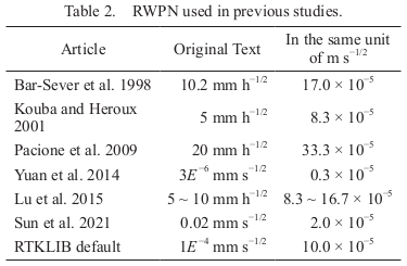
Zumberge et al. (1997) found that treating the ZTD time variation as a stochastic process is effective. The RWPN sigma constrains the degree of ZTD time variation. Optimum time ZTD constraint should be geographically and timely dependent. Several studies modeled ZTD as a random walk process and used their own RWPN settings, ranging from 0.3 × 10⁻⁵ m s^−1/2 to 33.3 × 10⁻⁵ m s^−1/2 (Table 2). The RTKLIB default RWPN sigma value is 10.0 × 10⁻⁵ m s^−1/2, which is set as a value that empirically gives the best result of the positioning solution. Vaclavovic et al. (2017) examined the impacts of the RWPN sigma of ZTD on estimated unknown parameters and observed a significant negative correlation between the estimated height and ZTD. They concluded that a careful offline analysis of an optimal RWPN setting for an estimated ZTD should be performed to achieve the best accuracy. Hadas et al. (2017) proposed using NWP models to define optimum RWPN settings.

Fig. 1.

Schematic illustration of two procedures of real-time analysis: (a) true real-time analysis, (b) rapid update of sliding window, and (c) postprocessing adopted by Shoji et al. (2017). In (b), the final (latest) time of the positioning analysis is the target time of the analysis. However, in (a) and (c), the target times of PWV analyses are within each GNSS analysis. In (c), data within 3 h from the start of each 27-h batch analysis were discarded to use well-converged results only; all the remaining 24-h results were treated as evaluation targets. In Shoji et al. (2017) and this study, when comparing with RAOB PWV, GNSS-derived PWV averaged 30 min from each RAOB launch time. For example, when compared with a RAOB launched at 11:30 UTC or 23:30 UTC, the GNSS-derived PWV is the 30 min average value from 14.5 h to 15 h or 26.5 h to 27 h after the analysis start time, respectively.

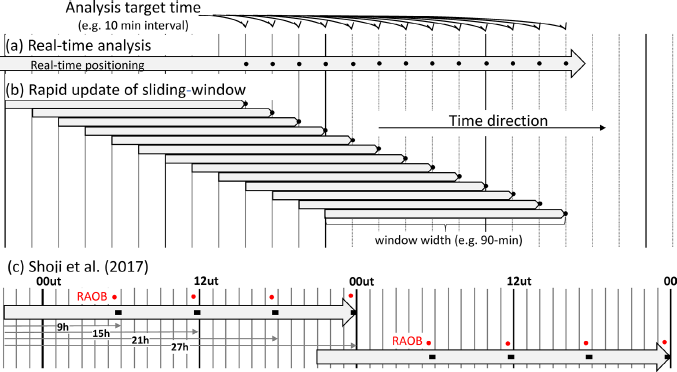
There are two options for real-time analysis: true real-time analysis, which continuously updates the forward analysis using information, such as satellite orbit and carrier phase obtained in real-time, or rapid update of sliding-window analysis (Foster et al. 2005), which frequently performs batch processing while updating the analysis target time. Figures 1a and 1b illustrate the differences between the two analysis procedures. Figure 1a is superior regarding computer load compared to (b) due to multiple estimation of time-dependent parameters at each epoch in (b). If the positioning accuracy improves or does not change with wider time width, then (a) is the best option. When performing the sliding-window analysis, appropriately determining the width of the sliding-window is necessary. The PPP analysis needs an order of tens of minutes of data to reach a converged solution (Choy et al. 2017). However, the wider the time width, the higher the computational cost. Foster et al. (2005) chose 8-h width to effectively compromise the processing time and solution accuracy. Shoji et al. (2017) adopted a traditional 24-h-batch approach (Fig. 1c), but with an extra 3 h of data added before each 24-h data file to avoid using unconverged solutions.

Several studies suggested a high rate of up to 10 Hz for the GNSS analysis to monitor the dynamic behavior of engineering structures and seismology (Wang et al. 2012; Xu et al. 2013). However, Erol et al. (2020) investigated the effect of different sampling intervals on the PPP solutions and found that higher sampling rates produced solutions with relatively poor quality in kinematic PPP results. According to them, this could be due to the high temporal correlation between observations with a higher sampling rate caused by multipath and atmospheric errors.

The above three parameters may affect GNSS analysis differently, depending on their combination. However, a statistical inspection of all combinations is difficult partly due to the computational load. First, we selected the optimal RWPN setting. Second, we examined the combined effects of time width and update interval.

In Section 2, we compared the ship-based GNSS-derived PWV with those calculated from the grid point value (GPV) of MA. There was no combination of settings with the best agreement on following all three measures: the regression coefficient of the linear regression line, bias, and standard deviation (SD) of the differences. Subsequently, to compare with other observations in Section 3, we selected one set of the RWPN, the time width, and the update interval that resulted in one of the good agreements with MA.

2.1 Observation and PWV retrieval

Table 3 summarizes vessel sizes, weights, GNSS antennas, and receiver types. It displays the GNSS antenna on each vessel used herein. We conducted ship-based GNSS observations on one research vessel, Ryofu Maru, and two cargo ships, Wakanatsu, and Ryuunan, starting in December 2018. We initially set the evaluation period to about one month around the Japanese rainy season, June 15–July 15, 2020. Unfortunately, we could not conduct high-sampling observations on Ryofu Maru for operational reasons. Alternatively, we executed 10 Hz GNSS observations on Wakanatsu and Ryuunan from October 22 to November 20, 2020.

To acquire the ZTD time series every 30 min, using RTKLIB, kinematic PPP analyses with the sliding-window method were conducted. To calculate PWV from ZTD, Zenith Hydrostatic Delay (ZHD) was obtained, following Elgered et al. (1991), as a function of the pressure, latitude (φ), and altitude (ht) of the GNSS antenna.

  

Next, the zenith wet delay (ZWD) is derived by subtracting ZHD from ZTD.

  

Finally, PWV was estimated from ZWD using a conversion coefficient (Π) (Askne and Nordius 1987).

  

  

where R_v, M_w, and M_d are gas constant for water vapor, molecular weight of water vapor, and molecular weight of dry air. k₁, k₂, and k₃ are empirical constants for refractivity formula. T_m indicates the mean temperature of the atmospheric column weighted by the amount of water vapor defined by Davis et al. (1985).   

where H, T, and P_v are GNSS antenna height, temperature, and vapor pressure, respectively. Bevis et al. (1992) indicated that T_m correlates with surface temperature. This parameter is estimated from the interpolated surface temperature, using a linear relation between T_m and surface temperature based on one-year statistics of RAOB in Japan.

Therefore, to calculate PWV from ZTD obtained in GNSS positioning, P and T value at the GNSS antenna position are required. From Subsection 2.2–2.4, MA's GPV interpolated to the GNSS antenna location was used for the P and T values. Section 3 used the P and T values observed on each vessel. We compared the PWV calculated using the P and T of MA with those using the observed P and T for one month of April 2021. The correlation coefficient of the two sets of PWVs exceeded 0.999, the absolute value of the mean difference was 0.11 mm, and the random difference was 0.2 mm.

The PWV of the MA was calculated by vertically integrating specific humidity.

  

where q, P, P_t, P_s, and g correspond to specific humidity, pressure, model top pressure, model surface pressure, and gravitational acceleration, respectively.

2.2 Examination of RWPN setting using Ryofu Maru data

To examine the optimal RWPN setting, eight GNSS analyses were performed for approximately 1 month (from June 15 to July 15) using 1 Hz-sampled Ryofu Maru data while changing the RWPN sigma as 1 × 10⁻⁴, 5 × 10⁻⁵, 3 × 10⁻⁵, and 1 × 10⁻⁵ m s^−1/2 and the time width of the sliding window as 1.5 h, and 8.0 h.

The RTKLIB default value for RWPN sigma is 1 × 10⁻⁴ m s^−1/2. The PWV time sequence of Ryofu Maru in Shoji et al. (2017) showed short-term fluctuations, which did not occur for PWV analysis with the static PPP of a nearby ground-based fixed GNSS station. Regarding the suppression of unnatural short-term fluctuations, we examined stronger RWPN constraints, and a detailed evaluation of the influence of the time width is presented in the next section. We compared the results of the two time widths of 1.5 h and 8.0 h. The former width was selected because Choy et al. (2017) mentioned that several tens of minutes are needed for PPP to converge, and the latter was selected based on Foster et al. (2005).

Table 4 and the scatter diagrams in Fig. 2 depict the comparison results of PWVs obtained from the eight experiment analyses against those by MA. To examine the differences in the agreement between cases with high and low PWV, the bias, RMS, and SD were calculated for three bins: (1) all data, (2) PWV < 40 mm, and (3) PWV ≥ 40 mm. For all data, the RMS difference and SD were smaller in the 1.5 h width, with a combination of the RWPN of 3 × 10⁻⁵ m s^−1/2. Conversely, the 8.0 h width tended to have larger RMS and SD values. This tendency seems to be stronger in smaller RWPNs. Regardless of the time width of the analysis or the selected RWPN setting, biases were positive for PWV < 40 mm and negative for PWV ≥ 40 mm. Comparing the RMS of the 1.5 h analysis with that of 8.0 h analysis, the positive biases for PWV < 40 mm and negative biases for PWV ≥ 40 mm tend to be closer to zero for the 1.5 h analysis. The selection of smaller RWPN (stronger time constraint) resulted in a larger positive bias for PWV < 40 mm and smaller negative bias for PWV ≥ 40 mm. The change in bias caused by using different RWPNs is greater for the 8.0 h analysis than for the 1.5 h analysis. As a result, for both 1.5 h and 8.0 h analyses, the selection of smaller RWPN resulted in smaller regression coefficients and larger y-intercepts of linear regression; however, it reduced the negative biases of GNSS-derived PWV. Comparing 1.5 h and 8.0 h analyses with the same RWPN shows that the former has a larger (closer to 1) regression coefficient and smaller y-intercept than the latter. While increasing the time constraint of the RWPN positively reduced the unnatural variability of the analyzed PWV, it also had a negative influence as reducing the regression coefficient and increasing the y-intercept of the linear regression line. Regarding the reduction of RMS in GNSS-derived PWV against MA, we can state that, among these eight experiments, a 1.5 h width with an RWPN of 3 × 10⁻⁵ m s^−1/2 showed the best agreement with MA.

Fig. 2.

Scatter diagram of PWV comparing MA and ship-based GNSS, in (a) 1.5 h and (b) 8.0 h widths. GNSS-derived PWVs are plotted with different colors depending on RWPN sigma, as (black) 1.0 × 10⁻⁴, (blue) 5.0 × 10⁻⁵, (red) 3.0 × 10⁻⁵, and (green) 1.0 × 10⁻⁵ m s^−1/2.

The panels in Fig. 3 represent the PWV time series by RAOBs (red dots), expressed in MA (thick gray line) and GNSS-derived PWV (other colored lines). A setting of smaller RWPN increases the suppression of the GNSS-derived PWV time variation, and the tendency is stronger in the results of 8.0 h width than that of 1.5 h width.

Fig. 3.

The 24 h PWV sequence at Ryofu Maru from 12:00 UTC July 4 to 12:00 UTC July 5, 2020. The (a) 1.5 h and (b) 8.0 h widths are shown. Gray lines represent MA, while red dots represent RAOB. GNSS-derived PWVs are plotted with different colors depending on RWPN sigma as (black) 1.0 × 10⁻⁴, (blue) 5.0 × 10⁻⁵, (red) 3.0 × 10⁻⁵, and (green) 1.0 × 10⁻⁵ m s^−1/2.

Figure 4 shows the differences in the estimated altitude dependent on the time width and the RWPN. The smaller the RWPN, the higher the analyzed altitude, specifically in 8.0 h width analyses. As Vaclavovic et al. (2017) and Shoji et al. (2000) reported, zenith coordinate errors negatively correlate with errors in ZTD. Conversely, height overestimation occurs in synchronization with ZTD underestimation. The results shown in Figs. 2–4 indicate that (1) adopting an RWPN smaller than RTKLIB's default value yields smaller RMS and SD of GNSS-derived PWV, and (2) a smaller RWPN tends to create positive biases in the zenith coordinate. The biases increase with a wider time width.

Fig. 4.

The 24 h sequence of altitude at RYOFU MARU GNSS antenna from 12:00 UTC July 4 to 12:00 UTC July 5, 2020. The (a) 1.5 h and (b) 8.0 h widths are shown. Lines are plotted with different colors depending on RWPN sigma as (black) 1.0 × 10⁻⁴, (blue) 5.0 × 10⁻⁵, (red) 3.0 × 10⁻⁵, and (green) 1.0 × 10⁻⁵ m s^−1/2.

2.3 Examination of EKF update interval and time width

In kinematic PPP with the MADOCA real-time product, 30–40 min continuous data are required from the start time for the analysis to converge (Kogure et al. 2016). The sampling interval (time interval of update of EKF state vector) may affect the convergence time and positioning accuracy. Therefore, we experimented with an accuracy comparison using 10 Hz observation data while changing the time width and the update interval.

From October 22 to November 20, 2020, we conducted a dual-frequency 10 Hz sampling GNSS observations on two cargo ships, Wakanatsu and Ryuunan (Table 2). In the GNSS analysis, the RWPN was fixed at 3 × 10⁻⁵ m s^−1/2, based on Subsection 2.2. Subsequently, the time width of the sliding window was changed from 0.5 h to 8.5 h with a 1 h time slot, while the update interval was modified 13 times, from 0.1 s to 30 s. Using GNSS-estimated ZTD and the pressure and temperature of MA interpolated at the GNSS antenna position, the GNSS-derived PWV was estimated every 30 min to match the time interval of the MA dataset and subsequently compared with the MA PWV.

From the comparison (Fig. 5), we can observe the following characteristics:

1. (a) The regression coefficient of the linear regression line is the largest when the time width is 1.5 h and the update interval is 20 s. At update intervals exceeding 2 s, the regression coefficient becomes the largest at a time width of 1.5 h, but the regression coefficient becomes smaller as the update interval becomes shorter. The longer the update interval, the greater the regression coefficient change as the time width changes.
2. (b) The y-intercept of the linear regression line also varies with the time width and the update interval. The longer the update interval, the greater the change in the y-intercept with time width. At a time width of 1.5 h, the y-intercept becomes closest to zero (−0.36 mm) at an update interval of 2 s and becomes farthest from zero (−0.79 mm) at an update interval of 30 s. The longer the update interval, the greater the change in the y-intercept with time width.
3. (c) When the update interval is shorter than 10 s, negative bias increases with decreasing update interval and increasing time width. At a time width of 1.5 h, the negative bias becomes closer to zero than −1 mm when the update interval is between 2 s and 15 s and becomes the smallest (−0.89 mm) at an update interval of 4 s.
4. (d) SD becomes minimal at a time width of 1.5 h irrespective of update interval. The longer the update interval, the greater the change in the SD with time width. SD becomes the smallest (1.99 mm) for update intervals of 1 s and 2 s.
5. (e) The changes in RMS are similar to those in SD but reflect the influence of bias. The RMS is the smallest (2.19 mm) at an update interval of 4 s and the second smallest (2.20 mm) at an update interval of 2 s.

Fig. 5.

Different time widths of sliding windows (x-axis) and update intervals (line color) cause differences in ship-based GNSS-derived PWV comparison against MA. (a) The regression coefficient of the linear regression line, (b) y-intercept of the linear regression line, (c) bias, (d) SD, and (e) RMS. Lines are plotted with different colors depending on the update interval.

According to Fig. 5, the optimal time width that will minimize the SD and RMS is 1.5 h. However, determining the optimal update interval is difficult. No setting satisfies the linear regression line's regression coefficient and y-intercept. The negative y-intercept values tend to be larger in groups where the regression coefficient is close to 1, so the relative error becomes larger in a smaller PWV environment. Further, the groups with a regression coefficient close to 1 differ from those with smaller bias, SD, and RMS. In this study, we selected an update interval of 2 s because with a 2 s update interval, y-intercept and SD values were closest to zero, and RMS was the second closest to zero. With respect to bias, the update interval of 4 s is closest to zero. For the 4 s update interval, the regression coefficient was closer to 1 than that for the 2 s update interval, and the RMS was minimal. The choice of update interval may vary between 2 s and 5 s, depending on which of the five indicators shown in Fig. 5 is considered more important.

In summary, we selected the following combination of settings for comparisons with other observations in Section 3: an update interval of 2 s, a time width of 1.5 h, and an RWPN sigma of 3 × 10⁻⁵ m s^−1/2 (red line in Fig. 5).

3. Comparison with other observations

In this section, we present the differences in the results between the method proposed by Shoji et al. (2017) and the combination of settings chosen in Section 2 by comparing PWVs using ship-based GNSS with those using RAOB, a nearby ground-based fixed GNSS, and a satellite-borne microwave radiometer (SMWR).

We note that each piece of information has a different spatiotemporal scale when comparing GNSS-derived PWV with other observed or analyzed values. The GNSS-derived PWV can be regarded as an average value in an inverted conical space with a radius of approximately 30 km and the GNSS antenna at its apex. The RAOB data are often used as a reference value for evaluating remote sensing observations. However, it takes approximately 0.5 h to travel through the troposphere. Therefore, compared with RAOB, the GNSS-derived PWVs need to be averaged for approximately 30 min, which may obscure the effect of the unnatural PWV fluctuation mentioned by Shoji et al. (2017). Additionally, after launch, each radiosonde drifts with the wind. The SMWR is a remote sensing instrument for measuring weak microwave emissions from the Earth's surface and atmosphere. The SMWR-observed values are considered instantaneous values at the time of observation, and the spatial resolution depends on the observation beam width.

When the PWVs of ship-based GNSS are compared with those of RAOB, nearby ground-based fixed GNSS, and SMWR, certain characteristics regarding the ship-based GNSS-derived PWV accuracy are revealed. In the following comparison, we referred to the method of Shoji et al. (2017) as CTL and our method as NEW. To examine the differences in agreement between cases with high and low PWV, bias, RMS, and SD were calculated for three bins: (1) all data, (2) PWV < 40 mm, and (3) PWV ≥ 40 mm.

3.1 Comparison with RAOB

Figure 6 shows the PWV comparison results from the Ryofu Maru observation in 2019 and 2020. A total of 134 RAOBs were compared with the ship-based GNSS-derived PWVs. Following Shoji et al. (2017), GNSS-derived PWVs were time-averaged over 30 min beginning at each radiosonde launch time. Comparing NEW with CTL for all data, RMS and SD decreased by approximately 0.1 mm, although negative bias increased by 0.1 mm. In the bin of PWV < 40 mm, the negative bias increased by 0.2 mm, whereas the negative bias decreased by 0.04 mm in the bin of PWV ≥ 40 mm. As a result, the regression coefficient approached 1, but y-intercept turned negative.

Fig. 6.

PWV comparison results from Ryofu Maru observations in 2019 and 2020. In (a), the GNSS-derived PWV is retrieved using the procedure of Shoji et al. (2017), while the GNSS-derived PWV is retrieved by using our new settings, as shown in (b). Black lines are linear regression lines.

3.2 Comparison with a nearby ground-based GNSS station

Between March 22 and 26, 2021, wiring and equipment installation for permanent dual-frequency GNSS observation on two JMA research vessels, Ryofu Maru (call sign JGQH) and Keifu Maru (call sign JPBN), were performed. We started observations on March 26; they are still ongoing as of April 2023. The system overview, data acquisition statistics, and an observation case are in the Appendix.

The two vessels were anchored side by side at their homeport of Daiba, Tokyo, until they departed on April 7, 2021. From the PWV time sequences from April 1 to 6 (Fig. 7), we confirmed that the PWVs analyzed from both vessels agreed well with those of a nearby ground-based fixed GNSS station (3023) and the MA. The PWVs analyzed from ground-based fixed GNSS observations were assimilated into the MA. With CTL (Fig. 7b), fluctuations with a cycle of approximately several hours are conspicuous in the PWV time series of both JGQH and JPBN. The amplitude of the fluctuations often exceeds 5 mm.

Fig. 7.

The PWV time sequence for April 1–April 6, 2021. Gray thick line: MA. Black line: 3023 (nearby fixed GNSS station). Blue line: Ryofu Maru (JGQH); Red line: Keifu Maru (JPBN). All-time series are drawn using data at 30-min intervals. The time sequences of JGQH and JPBN in (a) are obtained by the new settings described in this study, while those in (b), written as CTL, are obtained by those of Shoji et al. (2017). During this period, the two vessels were anchored side by side at their home port (Daiba, Minato Ward, Tokyo). The GEONET station 3023 (Chiba Ichikawa) is located approximately 12 km ENE from JGQH and JPBN.

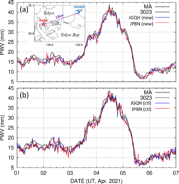
For April 1 to July 22, 2021, we compared PWVs of JGQH and JPBN with those of “3023” only when each vessel was within 15 km from “3023”. The results in Fig. 8 indicate that SD and RMS values are closer to zero in comparing all data with the NEW settings. The biases were positive for both JGQH and JPBN. The change in bias of the bin of PWV < 40 mm relative to the bin of ≥ 40 mm was −0.64 mm (JPBN) and −0.43 mm (JGQH) for CTL and −0.42 mm (JPBN) and +0.01 mm (JGQH) for NEW. The change in bias dependence on the PWV is smaller in NEW than in CTL.

Fig. 8.

PWV comparison between a ground-fixed GNSS station (3023) and ship-based GNSS on JPBN (red circles) and JGQH (blue triangles). Comparisons were made between April 1 to July 22, 2021, when each vessel was located within 15 km of the “3023” station. Linear regression lines are also plotted with red and blue lines.

3.3 Comparison with an SMWR

The Global Change Observation Mission (GCOM), a Japan Aerospace Exploration Agency project of long-term observation of environmental changes on Earth, launched its first satellite, GCOM-W1, on May 18, 2012. Advanced Microwave Scanning Radiometer 2 (AMSR2) uses 18.7, 23.8, and 36.5 GHz bands to observe PWV over the ocean for a horizontal resolution of approximately 15 km (Kazumori 2013).

We allowed a 5 min difference and a 20 km distance for the matchup, and Fig. 9 shows the comparison results. Concerning GCOM-W1, the GNSS-derived PWV has > 1 mm positive biases. Like the RAOB and ground-based fixed GNSS comparison, the PWV with NEW results in smaller SD and RMS values than CTL. The change in bias for PWV < 40 mm and ≥ 40 mm is also −1.90 mm (JPBN) and −1.72 mm (JGQH) for CTL. However, the analysis with NEW showed reduced changes of −1.31 mm (JPBN) and −1.08 mm (JGQH). Similar to the comparison with RAOB and ground-based fixed GNS station, the change in bias dependence on the PWV is smaller in NEW than in CTL.

Fig. 9.

GCOM-W1/AMSR2 with ship-based GNSS-derived PWV on JPBN (red circles) and JGQH (blue triangles). Comparisons were made between April 1 to July 22, 2021. When making comparisons, time differences of up to 5 minutes and differences in location within a distance of 20 km were allowed. Linear regression lines are also plotted with red and blue lines.

4. Discussion

In Section 3, we found the following:

1. a) The new analysis setting suppresses the unnatural fluctuation of ship-based GNSS-derived PWV observed by Shoji et al. (2017). Comparisons with RAOB, a nearby ground-based fixed GNSS station, and SMWR show a decrease in RMS and SD, except for RAOB with a PWV ≥ 40 mm.
2. b) Bias changes were characterized differently depending on the observations used for comparisons. The negative bias increased by about 0.1 mm in comparison to RAOB, the positive bias increased by 0.01 mm and 0.16 mm for JPBN and JGQH, respectively, in comparison to a ground-based fixed GNSS station, and the positive bias decreased by 0.13 mm and 0.1 mm in JPBN and JGQH, respectively, in comparison to SMWR. In all comparisons, the NEW setting showed smaller bias dependence on the PWV.

Herein, we discuss the bias in GNSS-derived PWV and its relation to the bias in estimated GNSS antenna height.

In GNSS positioning, a negative correlation between errors in analyzed heights and those in ZTD exists. Through geometric considerations, Beutler et al. (1988) derived the following relationship between errors in station height and those in ZTD:

  

where Δh, ΔZTD, and Z_max are the error in station height, error in ZTD, and maximum zenith angle (90-elevation angle) of GNSS satellites, respectively. By realistically considering receiver clock errors, Santerre (1991) found that errors in vertical coordinates and ZTD are negatively correlated. Rothacher and Beutler (1998) obtained the same results from independent derivations and analysis of observed data. Shoji et al. (2000) and Vaclavovic et al. (2017) also confirmed the negative correlation between the errors in the station height and ZTD. Here, we discuss the study results regarding the analyzed antenna heights.

Figure 10 shows a scatter plot of the analyzed altitude differences (CTL-NEW) and those in PWV for the data plotted in comparison with a nearby ground-based fixed GNSS station “3023” (Fig. 8). The correlation between the altitude and PWV differences was −0.4809 and −0.5072 for JPBN and JGQH, respectively. The linear regression lines implied that an overestimation in altitude of approximately 10 cm corresponds to an underestimation in PWV of about 1 mm, and vice versa.

Fig. 10.

Scatter plot and linear regression lines of the difference in analyzed altitude (CTL-NEW) versus the difference in PWV for the data plotted in Fig. 8.

Figure 11 shows the difference between the analyzed altitudes by CTL and NEW, using the comparison data of a nearby ground-based fixed GNSS station “3023.” The horizontal axis is the PWV at “3023”. The altitude differences were binned by PWV values at “3023” at 20 mm intervals and then averaged at each bin. The numbers at the top of each panel are the average differences in altitude at each bin. Although there is a large variation, increasing the PWV could elevate CTL's altitudes more than NEW's. For JPBN and JGQH, the elevation difference between the bin with a PWV ≥ 40 mm and the bin with a PWV < 20 mm is around 2 cm.

Fig. 11.

Differences in the analyzed GNSS antenna altitude using the settings of CTL and NEW (CTL-NEW) for the data plotted in Fig. 8. (a) JPBN and (b) JGQH.

Table 5 shows the expected PWV difference by applying the mean height difference between CTL and NEW to the linear regression equations (Fig. 10) for PWV < 40 mm and PWV ≥ 40 mm, respectively. From Fig. 8, the actual average PWV difference for JPBN was +0.02 mm when PWV < 40 mm and −0.20 mm when PWV ≥ 40 mm. The expected PWV difference of JPBN (Table 5) (+0.003 mm for PWV < 40 mm and −0.235 mm for PWV ≥ 40 mm) are consistent with the actual values. However, for JGQH, the actual difference is −0.06 mm for PWV < 40 mm and −0.50 mm for PWV ≥ 40 mm, while the expected value is −0.140 mm and −0.295 mm, respectively. Although there is a common tendency to increase negative differences with increased PWV, the expected values are not quantitatively consistent with actual PWV differences. Reflected GNSS signal waves in ship-based GNSS observations and changes in the phase center due to antenna tilt and rotation may have affected the results. Assessing the effects of these error factors inherent in ship-based GNSS observations is an issue to be addressed in the future.

To study the relationship between the errors in altitude and PWV, we installed a set of the same type of GNSS antenna and a receiver with that at Keifu Maru in a field at the Meteorological Research Institute (Tsukuba, Ibaraki, Japan) and conducted a 16-day GNSS observation from December 1 to December 16, 2021. We executed both static and kinematic PPP and compared the positioning results. The settings of kinematic PPP were changed as follows: (i) 16 time widths, from 0.5 h to 8.5 h, increased by 0.5 h each; (ii) five update intervals, 0.1, 1.0, 2.0, 10.0, and 30.0 s; and (iii) two RWPNs, 1 × 10⁻⁴, and 3 × 10⁻⁵ m s^−1/2. Table 1 presents other settings. Additionally, we performed a 16-day static PPP analysis using 24 h batch processing with precise ephemeris provided by the International GNSS Service (IGS). Hereafter, we refer to IGS's precise ephemeris as IGF. The update interval was set to 30.0 s to match the time interval of clock correction of the IGF, and the RWPN was set in two ways: 1 × 10⁻⁴ and 3 × 10⁻⁵ m s^−1/2.

Figure 12 shows the average and SD of the estimated altitudes when the RWPN of kinematic PPP was set to an RTKLIB default value, 1 × 10⁻⁴ m s^−1/2. The averaged altitude (25396.77 mm) and ±1 sigma (2.31 mm) altitudes from the static PPP analysis are also shown in the figure. When the time window was 0.5 h, the vertical coordinate average was lower than the average of the static PPP result, and the SD was larger than that of the wider time width. With increasing time width, the vertical coordinate average increases, and the SD reduces. If the update interval is 30 s and the time width is 4 h or above, the average altitude falls within the average altitude ±1 sigma of the static PPP. For update intervals shorter than 2 s, the analyzed mean altitude tends to increase with shorter update intervals and wider time widths. The SD of the analyzed altitude shows a smaller change when the time width ≥ 2 h compared to the change when the time width ≤ 1.5 h. Compared to the same time width, the shorter the update interval, the larger the SD. As Erol et al. (2020) noted, a reduced update interval does not necessarily appear to improve the accuracy of the positioning results.

Fig. 12.

Average and SD of analyzed altitudes of a fixed GNSS station at the Meteorological Research Institute (Tsukuba, Ibaraki, Japan) by kinematic PPP, applying the default value of RWPN, 1.0 × 10⁻⁴ m s^−1/2, for 16 d from December 1 to 16, 2020. In (a), a thick, gray horizontal line is the average of the daily analyzed altitudes (25396.77 mm) estimated by the static PPP applying the IGS precise ephemeris (IGF). The two black horizontal lines above and below the thick, gray horizontal line indicate the altitude of the average ± 2.31 mm SD.

Figure 13 is the same as Fig. 12, except that the RWPN is set to 3 × 10⁻⁵ m s^−1/2. For static PPP with IGF, changing the RWPN to 3 × 10⁻⁵ m s^−1/2 increased the mean altitude by about 0.5 mm, while the SD of the altitudes was almost the same. However, for update intervals ≤ 2 s, compared to Fig. 12, the analyzed altitude average tended to be higher, and SD tended to be smaller for shorter update intervals. For the kinematic PPP with an update interval of 2 s (red line), the average altitude with a time width of 1 h is closest to that of the static PPP (thick gray line). The average altitude for the 1.5 h width is 4.8 mm higher than that of the static PPP, and the altitude difference increases to 8.3 mm for the 2.5 h width. The SDs of the altitude were 58.6, 49.8, and 46.3 mm at time widths of 1.0, 1.5, and 2.5 h, respectively.

Fig. 13.

Same as Fig. 12, except the RWPN is 3.0 × 10⁻⁵ m s^−1/2. In (a), a thick, gray horizontal line is the average daily analyzed altitudes (25397.25 mm) estimated by the static PPP applying the IGF. The two black horizontal lines above and below the thick gray horizontal line indicate the altitude of the average ± 2.32 mm SD.

According to Kogure et al. (2016), 30–40 min of continuous data is needed for kinematic PPP convergence. From Figs. 12b and 13b, for the ship-based GNSS, about 2 h of continuous data is required for good convergence. In Fig. 5c, the SD is minimized for the 1.5 h width. This may be related to the positive bias in analyzed altitude, which increases with time width, and the degree of convergence of the kinematic PPP solution.

From Figs. 11 and 12, for 1.5 h width, smaller bias can be expected by 10 s update interval than by 2 s update interval. It is consistent with the features observed in Fig. 5c.

5. Summary and conclusions

In this study, we investigated the optimal real-time analysis settings for ship-based GNSS-derived PWV using the kinematic PPP function of RTKLIB. The results are summarized as follows:

1. 1) In kinematic PPP analysis, strengthening the constraint for ZTD time variation by setting the RWPN value up to one-third of the default value of RTKLIB suppresses the unnatural PWV time variation observed by Shoji et al. (2017). However, GNSS analysis with a smaller RWPN and longer analysis time resulted in a greater positive bias for PWV < 40 mm and greater negative bias for PWV ≥ 40 mm.
2. 2) Based on the results obtained by comparison of ship-based GNSS-derived PWV with MA PWV, a combination of an RWPN of 3 × 10⁻⁵ m s^−1/2, a time width of 1.5 h, and an update interval of 2 s were selected to compare with RAOB, nearby ground-based fixed GNSS, and SMWR measurements. Except for the comparison with RAOB when PWV was ≥ 40 mm, the SD and RMS values were smaller in all three comparisons than those obtained using the method of Shoji et al. (2017). The NEW setting showed a smaller bias dependence on the PWV in all comparisons. Our new analysis setting for ship-based GNSS PWV analysis was shown to reduce the growing negative bias of GNSS PWV under high PWV circumstances, which was one of the issues raised by Shoji et al. 2017.
3. 3) The biases in the GNSS-derived PWV described above were related to the biases in the vertical coordinate solutions using the kinematic PPP analysis. Errors in PWV based on GNSS analysis are negatively correlated with errors in vertical coordinates. In kinematic PPP analysis for a fixed ground-based GNSS station, positive biases occur in the vertical coordinate solution when the time interval of update is < 10 s. The biases increase with increasing time width and decreasing RWPN. Consequently, increased time widths, a strengthened constraint for ZTD time variation, and shorter update intervals may contribute to an increase in the negative bias of PWV.
4. 4) For update interval < 10 s, vertical coordinates tend to be underestimated at the initial stage of kinematic PPP analysis. The analyzed vertical coordinate increases with analysis time and tends to overestimate when the analysis time exceeds approximately 1 h. The SD of the vertical coordinate decreases with analysis time until it reaches approximately 2 h. The time width of 1.5 h was the time when the bias and SD of the vertical coordinate solution were both close to zero.

The present study allowed us to improve the method of Shoji et al. (2017) for PWV analysis using ship-based GNSS measurements. We suggest that the improvement in PWV analysis accuracy by ship-based GNSS is closely related to the improvement in vertical positioning accuracy. There is still scope for improvement in the vertical coordinate analysis and atmospheric delay in the kinematic PPP. However, we could not find a setting that yields the optimal values for all five measures: regression coefficient, y-intercept, bias, SD, and RMS. We evaluated the results from the analysis with a time width of < 9 h, although an increased analysis time width (≥ 24 h) might provide different results. Thus, future research should consider evaluating wider analysis times, including true real-time analysis. The cause of the error and the magnitude of its effect would vary depending on the observation environment, such as multipath, amount of water vapor and inhomogeneity, satellite arrangement, and sea conditions. The optimal PWV analysis setting for ship-based GNSS might differ depending on the above conditions. We think comparing with other observations and numerical weather models is necessary to find the optimal analysis setting for each observation environment. The present study provides an approach to searching for the optimal setting. The method for the adaptive setting of analysis options according to the observation situations could also be a future research subject.

Acknowledgments

We express our sincere gratitude to two anonymous reviewers and Professor Shunji Kotsuki for their essential comments that enabled us to carefully examine this study's purpose, procedure, and findings. A part of the RAOB was supported by the Cross-ministerial Strategic Innovation Promotion Program (SIP), “Enhancement of societal resiliency against natural disasters” (Funding agency: Japan Science and Technology Agency), and by JSPS KAKENHI grant 20H02420. The GEONET observation data and IGS precise ephemeris were acquired from the FTP server of the Geospatial Information Authority of Japan (GSI). We would like to thank Japan Fisheries Research and Education Agency, MarusanKaiun Co., Ltd., Ryukyu Kaiun Kaisha, KANIYAKU Co., Ltd. and MKKLINE Co., Ltd. for their cooperation for our ship-based GNSS observations. The authors would like to express their sincere appreciation to those who have made efforts to realize this real-time PWV analysis system over the ocean.

Data Availability Statements

The datasets generated and analyzed in this study are available from the corresponding author upon reasonable request.

APPENDIX

System overview, data acquisition statistics, and observation example for a heavy rain case of our real-time PWV analysis utilizing ship-based GNSS measurements.

A.1 System overview

Table A1 summarizes the vessels and equipment used for real-time PWV estimation. Our real-time positioning analysis at sea was possible since QZSS delivers MADOCA real-time products as one of its positioning signals (L6E). The Global Positioning Augmentation Service Corporation (GPAS) produced the MADOCA data delivered by QZSS. We installed Chronosphere-L6 GNSS receivers to receive the QZSS's L6E signal, and decode the MADOCA real-time orbit. The QZSS comprised three satellites in Quasi-zenith Orbits (QZO), and one satellite in Geostationary Orbit (GEO). To lengthen QZSS observation time from Japan, the QZO adopts an asymmetric north–south orbit shaped like a figure “8” centered around 135°E. Three QZO satellites can be observed every 8 h with an elevation angle of 70° or more in the Tokyo metropolitan area. However, as of August 2021, MADOCA on the L6E signal is transmitted from one GEO (QZS-3) and two out of three QZOs (QZS-2 and QZS-4), while the first QZO (QZS-1) did not transmit the L6E signal. Therefore, depending on the time of the day, receiving L6E becomes difficult because the elevation angle of all QZSSs (except QZS-1) will be below. The missing rate of the L6E signal increases as the receiver moves away from Japan in a direction other than the south.

The PC analysis collects the MADOCA real-time orbit and the career phase from GPS, GLONASS, and QZSS satellites. Following the results described in Section 2, it performs kinematic PPP analysis every 10 min. The RWPN, the width of the sliding window, and the update interval were set as 3 × 10⁻⁵ m s^−1/2, 1.5 h, and 2 s, respectively. The GNSS analysis was completed within 2 min from the start of each analysis.

Both vessels were equipped with JMA-certified meteorological sensors. We estimate PWV every 10 min with a latency of approximately 2 min by using GNSS-estimated ZTD and the observed temperature and atmospheric pressure on board.

A.2 Data acquisition statistics

Immediately after the system installation, minor corrections were required, such as setting the PC to always operate and acquiring meteorological observation data through the inboard data network. After making those corrections, the GNSS real-time analysis became stable by March 31. Since then, continuous analysis has been carried out regardless of whether vessels were moored or sailing.

From July 23 to August 5, 19 d of unscheduled outages and accuracy degradation of MADOCA occurred: According to the GPAS announcement, the cause was a problem in collecting global ground GNSS observation network data used to analyze GNSS satellite orbits and clocks. In this study, we set the validation period for 113 d from April 1 to July 22.

Table A2 summarizes the number and rate of successful PWV analyses and those of missing cases. For Ryofu Maru (JGQH), the most common cause of PWV analysis failure was an unexpected 20 h sleep of PC analysis, followed by the failure to acquire the L6E signal. For Keifu Maru (JPBN), there were many L6E reception failures, which were ∼ 2.5 %; the unexpected outage of the MADOCA real-time orbit also caused 17 cases.

Figure A1 illustrates the retrieved PWV distribution along the trajectories of the two vessels and the locations where the MADOCA acquisition failed. Compared to JGQH, JPBN sailed further north and east of Japan. For both ships, MADOCA acquisition often failed when the ships sailed in these directions. Figure A2 shows that in JPBN, the MADOCA acquisition often fails around 12:00–15:00 UTC. This coincides whenever the elevation angles of the two L6E transmitting QZSs (SV02 and SV04) are below 40°. The fact that the L6E signal is not transmitted from the first quasi-zenith satellite (SV01) leads to missing data in a specific time zone, especially for JPBN. The successor to SV01, launched on 26 October 2021, is designed to transmit the L6E signal. The number of missing data has been reducing since the operation start of the successor satellite on March 24, 2022.

Fig. A1.

Estimated GNSS-derived PWV along the trajectories of (a) Ryofu Maru (JGQH) and (b) Keifu Maru (JPBN). Pairs of red crosses and red circles are the start and endpoints of MADOCA acquisition failure.

Fig. A2.

Histogram of the number of MADOCA acquisition failures for the bins of time of day.

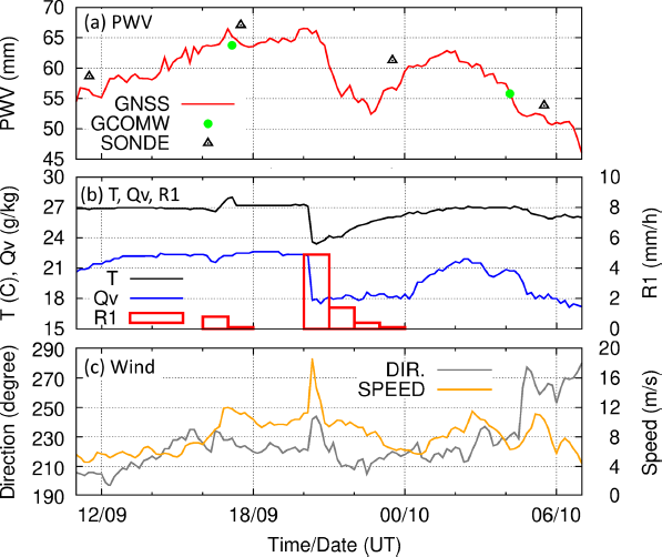
A.3 Heavy rain case between July 9 and July 10, 2021

Between July 9 and July 10, there was heavy rain in southern Kyushu. At the Satsuma Kashiwabaru weather station in Kagoshima prefecture in southern Kyushu, 24 h precipitation of 473 mm was recorded until 12:40 (local time, UTC +9 h) on July 10, and heavy rain emergency warnings were issued to Kagoshima, Miyazaki, and Kumamoto prefectures. The JPBN conducted RAOBs at 6 h intervals for 7 d, from July 5 to July 12, including the day with heavy rain. The PWV time sequence shown in Fig. A3 shows a rapid increase in PWV after 18:00 UTC on July 7 and a rapid decrease in the first half of July 10. Figure A3 also shows the short time variation in PWV, such as a 10 mm decrease followed by an increase of ∼ 5 mm in 6 h from 18:00 UTC on July 9, for which the 6 h interval observation could not be captured. The panels in Fig. A4 show the 20 h time sequence, from 11:00 July 9 to 07:00 July 10, 2021, of GNSS-derived PWV and surface meteorological data. The GNSS-derived PWV decreased by 10 mm or more in approximately 2 h from 21:00 to 23:00 on the ninth day. When GNSS-derived PWV began to decrease, sharp decreases in the temperature and mixing ratio, intensifying precipitation, and a large change in wind direction and speed were observed.

Fig. A3.

PWV sequence at Keifu Maru (JPBN) from July 5 to 12, 2021 (red line: GNSS; green circles: GCOM-W1; black open triangles: RAOB).

Fig. A4.

The 20 h time sequences of (a) PWV, (b) temperature, water vapor mixing ratio, 1 h precipitation, and (c) wind were observed on Keifu Maru from 11:00 July 9 to 07:00 July 10, 2021.

Figure A5 shows distributions of 1 h precipitation and PWV at 02:00 (local time, UTC +9 h) on July 10. Heavy rains exceeding 50 mm h⁻¹ in the southern part of Kyushu were analyzed. Heavy rain areas were channeled to the sea in the west–southwest direction. In GCOM-W1, a region with a PWV of more than 60 mm was detected along the heavy rain area. The JPBN is located near the western end of the heavy rainfall area.

Fig. A5.

Distribution of (a) radar/rain gauge analyzed precipitation (color shade), 7.3 µm band TBB by GMS HIMAWARI8 (gray shade), and surface wind (red vector), and (b) PWV analyzed from ground-based GNSS stations (larger dots on land), from GCOM-W1 (smaller dots over the ocean) and Keifu Maru (triangle) at 17:00 UTC on July 9, 2021.

These results indicate the potential of ship-based GNSS measurements to observe PWV at sea with high temporal resolution regardless of rain and to predict heavy rainfall.

References

•  Askne,  J., and  H.  Nordius, 1987: Estimation of tropospheric delay for microwaves from surface weather data. Radio Sci., 22, 379–386.
•  Bar-Sever,  Y. E.,  P. M.  Kroger, and  J. A.  Borjesson, 1998: Estimating horizontal gradients of tropospheric path delay with a single GPS receiver. J. Geophys. Res., 103, 5019–5035.
•  Bessho,  K.,  K.  Date,  M.  Hayashi,  A.  Ikeda,  T.  Imai,  H.  Inoue,  Y.  Kumagai,  T.  Miyakawa,  H.  Murata,  T.  Ohno,  A.  Okuyama,  R.  Oyama,  Y.  Sasaki,  Y.  Shimozu,  K.  Shimoji,  Y.  Sumida,  M.  Suzuki,  H.  Tanighuchi,  H.  Tsuchiyama,  D.  Uesawa,  H.  Yokota, and  R.  Yoshida, 2016: An introduction to Himawari-8/9— Japan's new-generation geostationary meteorological satellites. J. Meteor. Soc. Japan, 94, 151–183.
•  Beutler,  G.,  I.  Bauersima,  W.  Gurtner,  M.  Rothacher,  T.  Schildknecht, and  A.  Geiger, 1988: Atmospheric refraction and other important biases in GPS carrier phase observation. Atmospheric Effects on Geodetic Space Measurements. Monogr., No. 12, School of Surveying, Univ. of New South Wales, Kensington, Australia, 15–43.
•  Bevis,  M.,  S.  Businger,  T. A.  Herring,  C.  Rocken,  R. A.  Anthes, and  R. H.  Ware, 1992: GPS meteorology: remote sensing of atmospheric water vapor using the global positioning system. J. Geophys. Res., 97, 15787–15801.
•  Boehm,  J.,  B.  Werl, and  H.  Schuh, 2006: Troposphere mapping functions for GPS and very long baseline interferometry from European Centre for Medium-Range Weather Forecasts operational analysis data. J. Geophys. Res., 111, B02406, doi:10.1029/2005JB003629.
•  Boniface,  K.,  C.  Champollion,  J.  Chery,  V.  Ducrocq,  C.  Rocken,  E.  Doerfinger, and  P.  Collard, 2012: Potential of shipborne GPS atmospheric delay data for prediction of Mediterranean intense weather events. Atmos. Sci. Lett., 13, 250–256.
•  Burgos,  F. Y.,  P.  Alexander,  A.  de la Torre,  R.  Hierro,  P.  Llamedo, and  A.  Calori, 2018: Comparison between GNSS ground-based and GPS radio occultation precipitable water observations over ocean-dominated regions. Atmos. Res., 209, 115–122.
•  Chadwell,  C. D., and  Y.  Bock, 2001: Direct estimation of absolute precipitable water in oceanic regions by GPS tracking of a coastal buoy. Geophys. Res. Lett., 28, 3701–3704.
•  Choy,  S.,  S.  Bisnath, and  C.  Rizos. 2017: Uncovering common misconceptions in GNSS Precise Point Positioning and its future prospect. GPS Solutions, 21, 13–22.
•  Davis,  J. L.,  T. A.  Herring,  I. I.  Shapiro,  A. E. E.  Rogers, and  G.  Elgered, 1985: Geodesy by radio interferometry: Effects of atmospheric modeling errors on estimates of baseline length. Radio Sci., 20, 1593–1607.
•  Dee,  D. P., 2005: Bias and data assimilation. Quart. J. Roy. Meteor. Soc., 131, 3323–3343.
•  Elgered,  G.,  J. L.  Davis,  T. A.  Herring, and  I. I.  Shapiro, 1991: Geodesy by radio interferometry: Water vapor radiometry for estimation of the wet delay. J. Geophys. Res., 96, 6541–6555.
•  Erol,  S.,  R. M.  Alkan,  İ. M.  Ozulu, and  V.  Ilçi, 2021: Impact of different sampling rates on precise point positioning performance using online processing service. Geo-spatial Inf. Sci., 24, 302–312.
•  Foster,  J.,  M.  Bevis, and  S.  Businger, 2005: GPS meteorology: Sliding-window analysis. J. Atmos. Oceanic Technol., 22, 687–695.
•  Fujita,  M.,  F.  Kimura,  K.  Yoneyama, and  M.  Yoshizaki, 2008: Verification of precipitable water vapor estimated from shipborne GPS measurements. Geophys. Res. Lett., 35, L13803, doi:10.1029/2008GL033764.
•  Fujita,  M.,  T.  Fukuda,  I.  Ueki,  Q.  Moteki,  T.  Ushiyama, and  K.  Yoneyama, 2020: Experimental observations of precipitable water vapor over the open ocean collected by autonomous surface vehicles for real-time monitoring applications. SOLA, 16A, 19–24.
•  Hadas,  T.,  F. N.  Teferle,  K.  Kazmierski,  P.  Hordyniec, and  J.  Bosy, 2017: Optimum stochastic modeling for GNSS tropospheric delay estimation in real-time. GPS Solutions, 21, 1069–1081.
•  Huang,  C.-Y.,  W.-H.  Teng,  S.-P.  Ho, and  Y.-H.  Kuo, 2013: Global variation of COSMIC precipitable water over land: Comparisons with ground-based GPS measurements and NCEP reanalyses. Geophys. Res. Lett., 40, 5327–5331.
•  Ikuta,  Y.,  H.  Seko, and  Y.  Shoji, 2021: Assimilation of ship-borne precipitable water vapour by the Global Navigation Satellite Systems for extreme precipitation events. Quart. J. Roy. Meteor. Soc., 148, 57–75.
•  Imada,  Y.,  H.  Kawase,  M.  Watanabe,  M.  Arai,  H.  Shiogama, and  I.  Takayabu, 2020: Advanced risk-based event attribution for heavy regional rainfall events. npj Climate Atmos. Sci., 3, 37, doi:10.1038/s41612-020-00141-y.
•  Kato,  T., 2006: Structure of the band-shaped precipitation system inducing the heavy rainfall observed over northern Kyushu, Japan on 29 June 1999. J. Meteor. Soc. Japan, 84, 129–153.
•  Kato,  T., 2018: Representative height of the low-level water vapor field for examining the initiation of moist convection leading to heavy rainfall in East Asia. J. Meteor. Soc. Japan, 96, 69–83.
•  Kato,  T.,  Y.  Terada,  K.  Tadokoro,  N.  Kinugasa,  A.  Futamura,  M.  Toyoshima,  S.  Yamamoto,  M.  Ishii,  T.  Tsugawa,  M.  Nishioka,  K.  Takizawa,  Y.  Shoji, and  H.  Seko, 2018: Development of GNSS buoy for a synthetic geohazard monitoring system. J. Disaster Res., 13, 460–471.
•  Kazumori,  M., 2013: Chapter 2: Descriptions of GCOM-W1 AMSR2 Level 1R and Level 2 Algorithms. Description of GCOM-W1 AMSR2: Level 1R and Level 2 Algorithms. NDX-120015A, Japan Aerospace Exploration Agency, 2-1–2-11. [Available at http://suzaku.eorc.jaxa.jp/GCOM_W/data/doc/NDX-120015A.pdf.]
•  Kogure,  S.,  M.  Endo,  M.  Miyoshi,  K.  Sato,  K.  Kawate,  T.  Takasu,  T.  Osawa, and  T.  Suzuki, 2016: Multi-GNSS advanced demonstration tool for orbit and clock analysis (MADOCA), the development result and its product utilization to automobile applications. Proceedings of 2016 Annual Congress (Spring) of the Society of Automotive Engineers of Japan, 56-1 (in Japanese).
•  Kouba,  J., and  P.  Heroux, 2001: Precise point positioning using IGS orbit and clock products. GPS Solutions, 5, 12–28
•  Lu,  C.,  X.  Li,  T.  Nilson,  T.  Ning,  R.  Heinkelmann,  M.  Ge,  S.  Glaser, and  H.  Schuh, 2015: Real-time retrieval of precipitable water vapor from GPS and BeiDou observations. J. Geod., 89, 843–856.
•  Pacione,  R.,  F.  Vespe, and  B.  Pace, 2009: Near Real-Time GPS Zenith Total Delay validation at E-GVAP Super Sites. Bollettino Di Geodesia E Scienze Affini, 1, 61–73. [Available at http://igs.oma.be/_documentation/papers/eurefsymposium2008/near_real_time_gps_zenith_total_delay_validation_at_e_gvap_super_sites.pdf.]
•  Rocken,  C.,  J.  Johnson,  T.  Van Hove, and  T.  Iwabuchi, 2005: Atmospheric water vapor and geoid measurements in the open ocean with GPS. Geophys. Res. Lett., 32, L12813, doi:10.1029/2005GL022573.
•  Rothacher,  M., and  G.  Beutler, 1998: The role of GPS in the study of global change. Phys. Chem. Earth, 23, 1029–1040.
•  Santerre,  R., 1991: Impact of GPS satellite sky distribution. Manuscripta Geodaetica, 16, 28–53.
•  Shoji,  Y., 2009: A study of near real-time water vapor analysis using a nationwide dense GPS network of Japan. J. Meteor. Soc. Japan, 87, 1–18.
•  Shoji,  Y.,  M.  Kunii, and  K.  Saito, 2009: Assimilation of nationwide and global GPS PWV data for a heavy rain event on 28 July 2008 in Hokuriku and Kinki, Japan. SOLA, 5, 45–48.
•  Shoji,  Y.,  K.  Sato,  M.  Yabuki, and  T.  Tsuda, 2016: PWV retrieval over the ocean using shipborne GNSS receivers with MADOCA real-time orbits. SOLA, 12, 265–271.
•  Shoji,  Y.,  K.  Sato,  M.  Yabuki, and  T.  Tsuda, 2017: Comparison of shipborne GNSS-derived precipitable water vapor with radiosonde in the western North Pacific and in the seas adjacent to Japan. Earth, Planets Space, 69, 153, doi:10.1029/2005GL022573.
•  Shoji,  Y.,  H.  Nakamura,  K.  Aonashi,  A.  Ichiki, and  H.  Seko, 2000: Semi-diurnal and diurnal variation of errors in GPS precipitable water vapor at Tsukuba, Japan caused by site displacement due to ocean tidal loading. Earth, Planets Space, 52, 685–690.
•  Sun,  P.,  K.  Zhang,  W.  Suqin,  W.  Moufeng, and  L.  Yun, 2021: Retrieving precipitable water vapor from real-time precise point positioning using VMF1/VMF3 forecasting products. Remote Sens., 13, 3245, doi:10.3390/rs13163245.
•  Takasu,  T., 2013: RTKLIB 2.4.2 manual. 183 pp. [Available at http://www.rtklib.com/prog/manual_2.4.2.pdf.]
•  Teng,  W.-H.,  C.-Y.  Huang,  S.-P.  Ho,  Y.-H.  Kuo, and  X.-J.  Zhou, 2013: Characteristics of global precipitable water in ENSO events revealed by COSMIC measurements. J. Geophys. Res.: Atmos., 118, 8411–8425.
•  Tsuguti,  H., and  T.  Kato, 2014: Contributing factors of the heavy rainfall event at Amami-Oshima Island, Japan, on 20 October 2010. J. Meteor. Soc. Japan, 92, 163–183.
•  Vaclavovic,  P.,  J.  Dousa,  M.  Elias, and  J.  Kostelecky, 2017: Using external tropospheric corrections to improve GNSS positioning of hot-air balloon. GPS Solutions, 21, 1479–1489.
•  Wang,  G.,  F.  Blume,  C.  Meertens,  P.  Ibanez, and  M.  Schulze, 2012: Performance of high-rate kinematic GPS during strong shaking: Observations from shake table tests and the 2010 Chile Earthquake. J. Geodet. Sci., 2, 15–30.
•  Weiss,  J.-P.,  W. S.  Schreiner,  J. J.  Braun,  W.  Xia-Serafino, and  C.-Y.  Huang, 2022: COSMIC-2 mission summary at three years in orbit. Atmosphere, 13, 1409, doi:10.3390/atmos13091409.
•  Wick,  G. A.,  Y. H.  Kuo,  F. M.  Ralph,  T. K.  Wee, and  P. J.  Neiman, 2008: Intercomparison of integrated water vapor retrievals from SSM/I and COSMIC. Geophys. Res. Lett., 35, 3263–3266.
•  Xu,  P.,  C.  Shi,  R.  Fang,  J.  Liu,  X.  Niu,  Q.  Zhang, and  T.  Yanagidani, 2013: High-rate precise point positioning (PPP) to measure seismic wave motions: An experimental comparison of GPS PPP with inertial measurement units. J. Geodesy, 87, 361–372.
•  Yuan,  Y.,  K.  Zhang,  W.  Rohm,  S.  Choy,  R.  Norman, and  C.-S.  Wang, 2014: Real-time retrieval of precipitable water vapor from GPS precise point positioning. J. Geophys. Res.: Atmos., 119, 10044–10057.
•  Zhang,  Q.,  J.  Ye,  S.  Zhang, and  F.  Han, 2018: Precipitable water vapor retrieval and analysis by multiple data sources: Ground-based GNSS, radio occultation, radiosonde, microwave satellite, and NWP reanalysis data. J. Sens., 2018, 3428303, doi:10.1155/2018/3428303.
•  Zhou,  F.-C.,  X.  Song,  P.  Leng,  H.  Wu, and  B.-H.  Tang, 2016: An algorithm for retrieving precipitable water vapor over land based on passive microwave satellite data. Adv. Meteor., 2016, 1–11.
•  Zumberge,  J. F.,  M. B.  Heflin,  D. C.  Jefferson,  M. M.  Watkins, and  F. H.  Webb, 1997: Precise point positioning for the efficient and robust analysis of GPS data from large networks. J. Geophys. Res., 102, 5005–5017.