Abstract
Here, I create a dataset of fronts in mid- and high latitudes by applying an objective front detection method to the JRA-55 reanalysis and try climate classification based on dynamic climatology from temperate to polar regions. Additionally, I describe the interannual variations and long-term trends in the frontal zone. The unique feature of this study lies in the methods used for frontal data creation. This includes adding the geopotential height condition at 500-hPa to the conventional thermal-based objective method with equivalent potential temperature, including incorporating latitude-dependent parameters. The former increased the similarity between fronts created by the objective method and manually counted fronts on surface weather maps, while the latter enabled an examination of climate classification based on dynamic climatology by increasing the frontal frequency at high latitudes. The areas where climatic zones can be clearly defined are limited to the east of the great mountains in the mid-latitudes and the region where the Siberia-Canada Arctic frontal zone exists due to the obscuration or unclear seasonal movement of the frontal zones in other areas. The interannual variability in frontal zones is generally consistent with the characteristics of the regional climate variability associated with the El Niño Southern Oscillation, Pacific Decadal Oscillation, and Arctic Oscillation, as reported by previous studies. This study also reveals significant trends in some frontal zones since 1979, such as the northward shift in the eastern part of the North Pacific polar frontal zone during boreal autumn and winter and the decreasing frontal frequency on the northern coast of Norway in the European Arctic frontal zone from boreal winter to summer, including around the Beaufort Sea in the Siberia-Canada Arctic frontal zone in boreal summer.
1. Introduction
Frontal zones are recognized as areas where fronts are frequently depicted on daily surface weather maps. They climatologically correspond to the boundaries of air masses with different characteristics. Yazawa (1989) summarized early climatological studies of frontal zones. Bergeron (1930) first created a conceptual model of climatological frontal zones and air masses, considering the zone with frequent fronts as a frontal zone. This study attempts to understand the climate through atmospheric circulation dynamics. The locations of global major frontal zones have been identified based on the average atmospheric pressure or air stream on the surface (Petterssen 1940; Willett 1944; Chromow 1950), including fronts aggregation on surface weather maps (Reed 1960; Yoshimura 1967). Three global climatological frontal zones have been recognized from these results from the low to high latitudes: the inter-tropical convergence (ITCZ), polar frontal, and Arctic frontal zones. Furthermore, other individual features have been identified, e.g., some branches on the continent, including the Eurasian polar frontal zone and the obscurity of the Siberia-Canada Arctic frontal zone (SCAF) in boreal winter.
Alisov (1936) proposed that global climatic zones can be classified based on seasonal meridional variations in main frontal zones and the air masses and created the world climatic division map (Alissow 1954). The results have been criticized in some respects, i.e., climatic characteristics of each climatic zone, such as temperature and precipitation, are not shown and expressing the difference between continents and oceans needs criteria from another perspective. However, the structure of the global climatic zones in that study was known for its theoretical clarity.
Thus, frontal zones have been considered a straightforward concept for describing the state of the climate, and the importance of understanding their status and variability has been acknowledged. However, the frontal zones identified in these earlier studies contained data quality problems because they were drawn based on low temporal and spatial resolution ground observation data and insufficient high-level observation networks. Moreover, the objectivity of frontal zone data remains questionable: the definitions of frontal zones were vague and quantitative criteria were not established. The accuracy of Alisov's climatic divisions (Alisov 1936; Alissow 1954) also remains questionable, owing to issues, such as data quality, objectivity, homogeneity, and unclear criteria, in determining the location of the frontal zone. However, recent development has been conducted in research on methodologies to identify fronts using an objective approach, as will be discussed in subsequent paragraphs. The quality of the data for identifying fronts has also improved remarkably since the late 1970s compared to that in the mid-1900s, owing to developing objective reanalysis data from assimilated satellite information. Therefore, it is of great climatological interest whether the climate classification proposed by Alissow (1954) can be conducted based on recent objective frontal data; if so, how it can be expressed on global maps. This study aims to approach this issue by performing climate classification based on the annual movement of frontal zones in the mid- and high latitudes created by an objective front detection method.
Then, what objective method for creating frontal data should be selected to implement climate classification based on frontal zone behavior? Hewson (1998) summarizes several early studies on objective front detection methods. The work of Renard and Clarke (1965) is representative of early studies that examined objective methods for creating frontal data. This study used the thermal parameter, τ, such as temperature and various potential temperatures, and calculated the second derivative of τ as defined by
referred to as the thermal front parameter (TFP). We considered the front to locate the grid with a maximum value. The location of the maximum TFP is the warm side of the abrupt temperature decline, i.e., the edge of the warm air mass in the baroclinic zone, corresponding to the frontal location on the surface.
Clarke and Renard (1966) further attempted to improve the method to define the frontal location and introduce a thermal front locator where the derivative of the TFP is zero.
Hewson (1998) verified various methods using the TFP proposed by previous works [e.g., Huber-Pock and Kress 1981; Japan Meteorological Agency (JMA) 1988] and developed systematized frontal identification method: fronts are positioned by locating variables, third-order derivatives of τ, followed by excluding fronts below the thresholds of the masking variables, i.e., TFP (τ) and |∇τ|. Although this method provides specific threshold values for τ at 900-hPa and 600-hPa, the analyst selects the parameter settings for τ, such as physical quantity, pressure level, and each threshold, according to the region and data. In subsequent studies (e.g., Jenkner et al. 2010; Berry et al. 2011; Schemm et al. 2015; Parfitt et al. 2017), physical quantities θe (equivalent potential temperature) and θw (wet-bulb potential temperature), which include moisture information and imply rough equivalence (Bindon 1940; Berry et al. 2011; Thomas and Schultz 2019), and 925-hPa and 850-hPa pressure levels are often selected because they agree with the results of the manual frontal analysis. For the characteristics of the TFP (θe) distribution and frontal frequencies created using TFP (θe), Thomas and Shultz (2019) and Lagerquist et al. (2019) showed that frontal frequencies are high at low latitudes and low at high latitudes on global maps. Additionally, Schemm et al. (2015) pointed out the disadvantage of θe fronts, i.e., many quasi-stationary fronts appear in coastal and highland areas with a strong influence from moisture gradients.
In contrast, Simmonds et al. (2012) proposed an approach for detecting fronts based on temporal changes in the 10-m wind (hereinafter, “wind-based method”), different from the conventional method using temperature parameters (hereinafter, “thermal-based method”). Schemm et al. (2015) evaluated both methods based on comparing both characteristics over the globe and identified the following characteristics: The wind-based method can identify fronts even in weak baroclinic cases, but it tends to only identify cold fronts, whereas the thermal-based method (note that the front is set at the position where the TFP is zero) can identify long fronts with a larger zonal component, but it tends to identify many quasi-stationary fronts, as previously mentioned. Recently, Bitsa et al. (2021) presented a scheme for frontal identification using wind- and thermal-based methods. They accurately identified cold fronts with small spatial and temporal scales over the Mediterranean.
The significant developments in frontal identification methods focusing on wind- and thermal-based methods and objective reanalysis data (source for frontal identification) will allow for a more widely accepted unified expression of the frontal zone. However, the frontal identification method is still developing and requires further examination, especially with respect to drawing global frontal zones necessary for Alisov's climate classification. For example, compared to global distribution maps of frontal frequencies created by compiling fronts on weather maps (e.g., Yoshimura 1967; Matsumoto 1983), fronts created by the thermal-based method using θe as a thermal parameter are characterized by lower frontal frequencies in the polar region (e.g., Berry et al. 2011; Schemm et al. 2015). Although Serreze et al. (2001) identified fronts in polar regions using 850-hPa temperature as a thermal parameter, thermal parameters without moisture information are inappropriate for global frontal identification (e.g., Thomas and Shultz 2019). The global distribution maps of frontal zones created by the wind-based method (Schemm et al. 2015; Rudeva and Simmonds 2015) have the same low frequencies in the polar region. They also have a lower frontal frequency in Northern Hemisphere (NH) during summer than during winter almost anywhere in the NH. Furthermore, they cannot clearly identify the Baiu/Meiyu frontal zone, characterized by large moisture and small temperature gradients, with an expected high frequency around East Asia.
Evaluating the accuracy of objective fronts is difficult because it first involves the question “What is a front actually?” Sanders and Doswell (1995) and Sanders (1999) pointed out two major problems with fronts drawn on weather maps in forecast work: a lack of agreement among the analysts on detecting frontal existence and position and a lack of coincidence between fronts and the surface temperature field. They then argue for a definition of fronts corresponding to the mechanism of the phenomenon and the need for a detailed analysis of the surface temperature distribution. Evaluating objective fronts should be based on physical processes naturally, but this is not easily achieved at the present stage. While recognizing this problem, this study aims to create objective frontal data closely resembling fronts on surface weather maps and frontal zones on climate maps as a fundamental guideline to achieve the goal of climate classification. Thus, the study established various thresholds of masking variables for creating frontal data matching manually counted frontal data, as in many previous studies.
Based on the various objective front detection methods from previous studies, this study selected a slightly modified thermal-based method using θe as a thermal parameter (described below) rather than a wind-based method to create the frontal data. The idea of merging thermal- and wind-based methods, as proposed by Bitsa et al. (2021), is still developing and has not been validated, except in the Mediterranean. If we compare which method is better for climate classification using frontal zone based on the frontal frequency distribution in Schemm et al. (2015), a thermal-based method appears to identify frontal zones clearer in the mid-latitudes (including the Baiu/Meiyu frontal zone) with zonal extension than wind-based method. In Takahashi (2013), a method was studied for creating objective frontal data around Japan from NCEP/NCAR (National Centers for Environmental Prediction and the National Center for Atmospheric Research) Reanalysis-1 (Kalnay et al. 1996) using the thermal-based method for θ (potential temperature) and θe at 850-hPa. Therefore, creating frontal data using JRA-55 (Japanese 55-year reanalysis) in this study is positioned as an improved version of the method in Takahashi (2013), incorporating the results of trial and error when applying its method in identifying the frontal zone of the world.
First, I created frontal data around Japan following the method reported by Hewson (1998); however, I used θe at 850-hPa as a thermal parameter (θe at 850-hPa is often used for daily frontal analysis at the JMA and in research for detecting objective fronts). Additionally, although previous studies have set masking variables based on a single thermal parameter, this study attempted to incorporate the geopotential height at 500-hPa as masking variables by referring to the JMA frontal analysis. When drawing fronts on surface weather maps, the JMA referred to the maximum axis of the TFPs of the temperature thickness between 500-hPa and 850-hPa (Japan Meteorological Agency 1988). It now refers TFP (θe) at 925-hPa and 950-hPa, including an isotach at 300-hPa and geopotential height at 500-hPa, to observe how they correspond with the jet axis and upper trough (Japan Meteorological Agency 2018). This study did not consider information on the jet axis at 300-hPa because the spatial distance between the jet axis and front makes it difficult to establish the criteria. Second, I created global frontal data by incorporating a latitude-dependent parameter lowering the thresholds of the TFP (θe) and |∇θe| at high latitudes. Introducing this parameter is intended to compensate for the disadvantage of the θe fronts: the frontal frequency tends to be low at high latitudes. I then analyzed our frontal data and conducted climate classification in the mid- and high latitudes based on the annual movement of the polar and Arctic/Antarctic frontal zones. Specifically, climate classification was conducted by referring to the mean position of the frontal zones in January and February or in July and August, as in Alissow (1954).
As an additional survey, this study also investigated global frontal zones' interannual variability and long-term trends. While some objective methods for creating frontal data have been developed as mentioned above, a few studies have focused on interannual variations and long-term trends in global frontal zones, except for the study by Rudeva and Simmonds (2015), which examined the characteristics of frontal zone variability using a wind-based method. It is important to confirm these characteristics, such as the northward trend of frontal activity over the North Pacific in NH winter, from other frontal data, such as that in this study, to enhance the credibility of the trends.
In this study, various parameters were set based on statistical comparisons of distribution patterns to obtain a high similarity with manually counted fronts on surface weather maps. Through this process, we explore the possibility of climate classification via thermal-based methods. Although the numerical values of the parameters set in this manner are not physically meaningful, they can serve as a resource for considering the values of physical parameters in future studies.
2. Data and methods
2.1 Specific procedure for creating a dataset of fronts
This study used the JRA-55 to create a dataset of fronts. JRA-55 is publicly available at the JMA and has 6-hourly 1.25° latitude-longitude grid data since 1958 using an advanced data assimilation scheme (Kobayashi et al. 2015). Choosing the objective reanalysis product as a source of frontal data is important, especially since the spatial resolution relates to the threshold values of various parameters (e.g., Hewson 1998; Schemm et al. 2015). The highest spatiotemporal resolution global objective reanalysis data is currently ERA5 created by the European Centre for Medium-Range Weather Forecasts. ERA5 used an ensemble data assimilation method to achieve hourly 0.25° grid data since 1959 (Hersbach et al. 2020). This study used JRA-55 instead of ERA5 because the data had already been obtained and prepared for analysis, and the preliminary research for the parameter settings was already performed. JRA-55 has a slightly lower spatial resolution than ERA5, but this is not an issue because JRA-55 has a sufficient spatial resolution to draw synoptic-scale fronts. Thus, even the 1.25° grid data of JRA-55 hardly manage local fronts; however, applying a 3 × 3 spatial averaging filter resulted in smoother fronts and a better similarity to the manually counted fronts on surface weather maps, as will be described later. However, JRA-55 has humidity accuracy issues, so future studies require updated reanalysis data. The detailed procedure for creating frontal data is as follows.
-
1) The θe at 850-hPa was calculated using the formulas with relative humidity and temperature reported by Bolton (1980), and then spatially averaged on 3 × 3 grids. According to a preliminary case study, this spatial averaging filter should be applied to obtain a continuous front. The frequency of quasi-stationary fronts, which often appear in the θe fronts (e.g., Berry et al. 2011; Schemm et al. 2015), was also partially suppressed by applying this spatial filter. TFP (θe) and |∇θe| were derived for each grid based on the spatially averaged θe. While some studies (e.g., Schemm et al. 2015) have focused on grids with TFP = 0 using high-resolution data to determine the presence of the front, this study focused on grids with “a gradient of TFP” = 0 to set the threshold, which has been used in many studies. We note that in the preliminary case analysis, correspondence with weather map fronts around Japan when using “a gradient of TFP” = 0 was better than when using TFP = 0.
-
2) The zonal and meridional inclinations in the geopotential height at 500-hPa without applying a spatial average filter (hereinafter, δZ500-ew and δZ500-sn, respectively) were also incorporated as masking variables to determine the presence of a front. δZ500-ew and δZ500-sn are defined as the difference between the values of the adjacent grids to the east and west and the south and north of the grid of interest. Conditions for δZ500-ew and δZ500-sn values considered the characteristics of a surface front on the east side of the upper trough and that in the baroclinic zone, respectively. However, since the direction of the trough axis at high latitudes is often more north-south than that at mid-latitudes and inappropriate to apply thresholds of δZ500-ew and δZ500-sn, the threshold values of δZ500-ew and δZ500-sn were established only in the region above 5,700 gpm (low-latitude side).
-
3) After approximately estimating the threshold values in the case study analysis, multiple datasets of fronts were prepared by changing the threshold values of the TFP(θe), |∇θe|, δZ500-ew, and δZ500-sn by 0.01 K (100 km)−2, 0.01 K (100 km)−1, 1 gpm (100 km)−1, and 1 gpm (100 km)−1 increments around each estimated value, respectively. The position of the front on the weather map in the preliminary case study was used to compare the different datasets. The following adjustments were made to ensure the continuity of synoptic-scale fronts: First, to maintain the continuity of the front, if a front extends in an approximate west-east (including northeast-southwest and southwest-northeast) direction with a one-grid break, the gap is connected. Second, fronts with lengths of less than 800 km were deleted to eliminate localized fronts. The length of the front was estimated by calculating the length of the diagonal of the rectangle in the area containing the continuous front. Third, to smoothen the lines of possibly jagged fronts, the frontal position was shifted within one grid.
-
4) Each of these datasets of objective fronts was compared with the dataset of manually counted fronts compiled from the frontal analysis of JMA weather maps [hereinafter, F2009, created in Takahashi (2009)] and evaluated using the Jaccard index (hereinafter, JI) (Jaccard 1912), which measures similarity, as in the method of Takahashi (2013). Frontal data for F2009 were obtained by manually reading the position of the fronts from weather maps from April to November from 1979 to 2007, every 12 h at 10° longitude and 1° latitude. The JI was the value obtained from the intersection divided by the union of two datasets, and values close to 1 and 0 indicate high and low similarity, respectively. The JI was calculated for 10 years, from 1998 to 2007, in the region of 120–160°E and 25–40°N around Japan. If the frontal positions of the two datasets were within 5° of each other in the north–south direction, they were calculated as co-occurring. The advantage of the dataset of fronts obtained in this manner can be realized based on a comparison with the maximum JI of several datasets of fronts created under other conditions, i.e., fronts created with some conditions omitted and fronts created using NCEP/NCAR Reanalysis-1 with the method proposed by Takahashi (2013).
-
5) Finally, since detecting fronts using θe as the thermal parameter at high latitudes is difficult, I introduce the latitude-dependent parameter relaxing the threshold values of TFP (θe) and |∇θe| at high latitudes when creating global frontal data. Referring to the definition of a bomb cyclone using a change in surface pressure standardized to 60° (Sanders and Gyakum 1980), the threshold values of the TFP(θ e) and |∇θe| were standardized to 30° only for latitudes > 30°, indicating that each threshold value at each latitude (φ) was divided by sin φ/sin30° (φ > 30°).
The method for climate classification based on frontal zones was identical to that of Alisov's climate classification (Alissow 1954). Using data on monthly climatology averages from 1979 to 2020, the position of the northern/southern edge of the frontal zone (defined in two ways focusing on areas above a frontal frequency of 5 %, described later) in January and February and in July and August, was examined in each meridian. Climate classification was conducted based on the movement of the frontal zone position obtained in this manner; the results were superimposed and compared with those presented by Alissow (1954).
The interannual variabilities in the frontal zone on the global map were also analyzed in correlation with the El Niño Southern Oscillation (ENSO), Pacific Decadal Oscillation (PDO), and Arctic Oscillation (AO), which substantially impacts global climate variability. The indices representing each variation—the Niño-3 sea surface temperature (SST), PDO, and AO indices—were obtained from the NOAA CPC (Climate Prediction Center) website. Long-term trends in the distribution of frontal zones were evaluated using the Mann-Kendall test (Kendall 1975) derived from the 42-year frontal data from 1979 to 2020. The variation characteristics in the frontal zone revealed in this study were compared with the results reported by Rudeva and Simmonds (2015).
3. Global distribution of frontal zones
3.1 Effects of incorporating geopotential height at 500-hPa on frontal analysis
An example on 00Z 16 September 2007 was used to show how the newly added conditions related to the geopotential height at 500-hPa affect the detection of objective fronts. Here, I performed a case study in which the effects of the δZ500-ew and δZ500-sn indicators were observed. Frontal detection is often difficult in situations with adjacent typhoons because locally enhanced moisture gradients detect many local fronts. Matsuoka et al. (2019) attempted to detect stationary fronts using deep learning. They emphasized that the accuracy of frontal detection decreases in case of an approaching typhoon. Figure 1a shows a small weather map around Japan quoted from the JMA while Fig. 1b shows the distribution of objective fronts simultaneously created using the method described in Section 2. In Fig. 1b, the objective fronts created by the three different methods are plotted. The red circles indicate the grids (frontal position) that satisfied the conditions for four masking variables: |∇θe| > 0.55 [K (100 km)−1], TFP (θe) > 0.91 [K (100 km)−2], δZ500-ew > −6 [gpm (100 km)−1], and δZ500-sn > 3 [gpm (100 km)−1] (hereinafter, F2023). The orange and magenta circles mean the same as F2023, except for removing the δZ500-sn or δZ500-ew conditions (hereinafter, F2023b1 and F2023b2, respectively). Figure 1b also shows the contours of θ e at 850-hPa and geopotential height at 500-hPa.

A comparison of Figs. 1a and 1b reveals that the front under the F2023 conditions in Fig. 1b was the most similar of the three objective fronts to the front on the weather map shown in Fig. 1a. In this case, the typhoon was located at 32°N, 127°E. Under the F2023b1 conditions, fronts were observed on the southwest and northeast sides of the typhoon while they were not observed on the JMA surface weather map or in the F2023 conditions considering the north–south pressure gradient by adding the δZ500-sn condition. Conversely, the F2023b2 conditions analyzed fronts on the west side of the trough extending south-westward from 55°N and 150°E at 500-hPa, not shown on the JMA surface weather map or in the F2023 conditions, considering the east-west location of the trough via adding the δZ500-ew condition. As in this case, extra depicted fronts were removed by incorporating the δZ500-sn and δZ500-ew conditions, resulting in a higher similarity between the objective and weather map fronts.
Table 1 lists the maximum JI calculated between the dataset of F2009 and several datasets of objective fronts created under different reanalysis data and conditions. Table 1 also lists the thresholds for the thermal parameters and geopotential height for each dataset at a maximum JI. The first two capital letters of the dataset name indicate the name of the reanalysis data, where “NR” represents NCEP/NCAR Reanalysis-1 and “JR” represents JRA-55 reanalysis. For lower-case letters, “p” and “e” indicate that θ and θe were used as thermal parameters, respectively, “s” indicates that the spatial filters of the average of nine grids were adopted for thermal parameters in advance, and “g” indicates that data for the geopotential height at 500-hPa were used as additional conditions.

A comparison between JR-p and JR-e showed that the maximum JI of JR-e was higher than that of JR-p, indicating that θe was more competent than θ as a thermal variable for detecting frontal zones, as shown in previous studies (Hewson 1998; Jenkner et al. 2010; Schemm et al. 2015). Furthermore, a comparison of JR-e, NR-e, and JR-es, i.e., the spatial resolution and necessity for spatial filtering, showed that JR-es had the highest maximum JI of 0.537, whereas JR-e had a lower maximum JI than NR-e with a low resolution, implying that, for high-resolution reanalysis data, applying spatial filters should be considered before calculating parameters. In conclusion, JR-esg, which adds the 500-hPa geopotential height condition to JR-es, has the highest similarity of 0.587. Thus, adding the conditions for the geopotential heights, δZ500-ew and δZ500-sn, effectively created objective fronts similar to fronts around Japan on the weather map.
3.2 Effects of incorporating latitude-dependent parameters on global frontal data
Figure 2a shows the annual mean frontal frequency distribution calculated using the JR-esg averaged over the 42 years from 1979 to 2020. From Fig. 2a, the polar frontal zones in the mid-latitude ocean (North and South Pacific and South and North Atlantic) could be detected as areas with distinct high frontal frequency of ≥ 4 %. Conversely, although a simple comparison cannot be made owing to the different methods used to calculate frontal frequencies, the frontal frequencies in high-latitude areas in Fig. 2a are remarkably smaller than those shown in the maps of frontal frequencies presented by Yoshimura (1967) and Matsumoto (1983), calculated through manually counted fronts from weather maps. Previous studies using objective methods with temperature or θ at 850-hPa as the thermal parameter (not including moisture information) have also distinctly detected the Arctic fronts (Serreze et al. 2001; Renard and Clarke 1965). Berry et al. (2011), Thomas and Schultz (2019), and Lagerquist et al. (2019) also showed that the frontal frequency obtained using θe (or θw) was smaller at higher latitudes; therefore, applying the same conditions as those in the mid-latitudes when detecting fronts at high latitudes using θe appears inappropriate.

In contrast, Fig. 2b shows the annual mean frontal frequency distribution for the same period as that in Fig. 2a, obtained by incorporating the latitude-dependent parameter discussed in Section 2. Figure 2b shows that the Arctic/Antarctic frontal zones in the high latitudes were detected as clearly as the polar frontal zones in the mid-latitudes, compared with Fig. 2a. We could not determine whether the parameters incorporated in this study were the most appropriate. However, at least a relaxation of conditions by the latitude-dependent parameters for frontal detection allowed the identification of the front zones at high latitudes even when using θe or θw.
4. Seasonal transition of global frontal zone and trial of climate classification based on dynamic climatology
4.1 Mean seasonal transition of the global frontal zone
Figure 3 shows the three-month mean transition in the frontal frequency. Here, localized areas of quasi-stationary high frontal frequency occur at the land and sea boundaries, including mountainous areas, especially above 1,500 m (gray areas, 850-hPa in standard atmosphere), as indicated in Schemm et al. (2015). However, as this study focuses on the migrating frontal zone associated with the seasonal progression of the global atmospheric circulation, such as the polar and Arctic frontal zones, we did not consider such quasi-stationary fronts associated with orographic features for discussion.
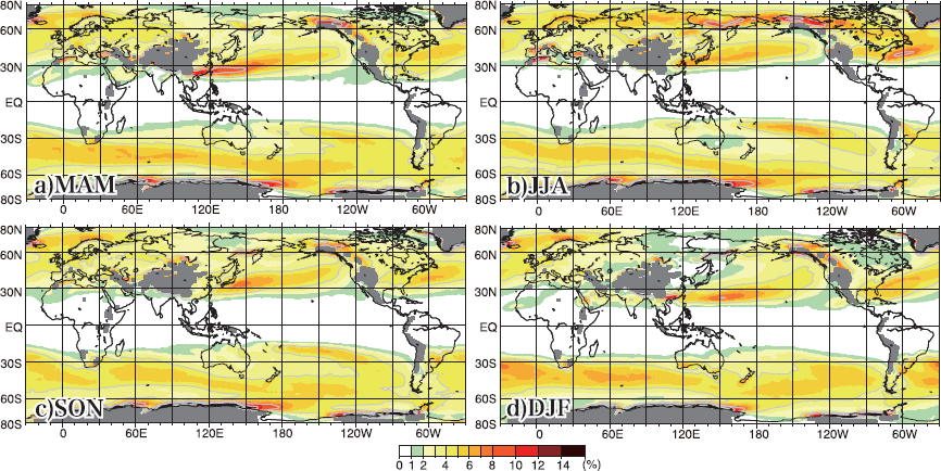
The overall characteristics of the frontal frequency distribution around the mid-latitudes were similar to those presented in previous studies using objective fronts created by the thermal-based method using θe (or θw) (Berry et al. 2011; Schemm et al. 2015; Thomas and Schultz 2019). Focusing on the NH, for instance, the North Pacific polar frontal zones (NPPF) and North Atlantic polar frontal zones (NAPF) were clearly observed in the mid-latitudes as regions with year-round frontal frequencies of ≥ 4 %, which also appeared in the annual mean in Fig. 2b. These polar frontal zones have a distinct seasonal migration in the time-latitude profiles around these areas (not shown), with a gradual shift to high latitudes during the warm season and low latitudes during the cold season. Figure 3 clearly shows the frontal zones around East Asia, vaguely identified by the wind-based method (Schemm et al. 2015; Rudeva and Simmonds 2015).
As for the frontal zones at high latitudes, in northern Europe around 65–75°N and 30°W–60°E, high-frequency areas corresponding to the European Arctic frontal zone were observed year-round, but the seasonal migration of the high frontal frequency areas was not large. Meanwhile, a large seasonal difference was found in the region from Eurasia to Canada, where a distinct frontal zone (SCAF) was observed in boreal summer but not in winter; this corresponds to the characteristic reported by Reed (1960) and Yoshimura (1967).
For the Southern Hemisphere (SH), three distinct and long-lined frontal zones were observed, i.e., the South Pacific Convergence Zone (SPCZ), the frontal zone extending in an east-southeast direction from east of the Andes Mountains (called the South Atlantic Convergence Zone; SACZ), and the frontal zone across the Southern Ocean from the south of Africa to the south of New Zealand. The latter two frontal zones appear connected in SH autumn and winter (Figs. 3a, b). The convergence zones of the SPCZ and SACZ in the subtropical region are known to have the characteristics of the subtropical frontal zone with a large vapor gradient like that of Baiu/Meiyu frontal zone (Kodama 1992).
Based on the comparison between the SH winter (Fig. 3b) and SH summer (Fig. 3d) and the time-latitude profile of SH frontal frequency (not shown), SH frontal frequencies were generally higher in SH summer than in SH winter. Distinct northward-southward migration with seasonal progression was observed in the SACZ around the region east of the Andes Mountains. However, the east part of this frontal zone, continuing into the Atlantic Ocean and the south of African and Australian continents, did not show a large seasonal migration. The SPCZ can be clearly observed year-round, especially in SH winter. The SPCZ is generally characterized as being the most active during SH summer and inactive during SH winter, and its formation and maintenance mechanisms are involved by various factors, such as the diabatic heating from a tropical heat source, forced equatorial Rossby wave, the influence of subtropical flow, and eddy forcing from the extratropics (e.g., Matthews 2012; Haffke and Magnusdottir 2013). Vincent (1994) showed that this convergence zone exhibits different activity characteristics between the tropics on the west side and the subtropics on the east side. Figure 3 is considered to represent only the SPCZ characterized by baroclinicity. Therefore, this seasonal transition of SPCZ in Fig. 3 suggests that baroclinicity may substantially maintain the convergence zone in the subtropical region during SH winter when the SPCZ is relatively inactive. The localized frontal frequency maxima observed in Fig. 3 in southern South Africa and southern Australia are the frontal zones known as dry fronts without precipitation (Berry et al. 2011).
To summarize the seasonal transition of the distribution of the frontal frequencies globally, three polar frontal zones, NPPF and NAPF in the NH and SACZ in the SH, were identified with distinct seasonal migration, and all located in the downstream region of large mountains. These frontal zones are characterized by a larger pole-ward shift in the eastern area during the cold season than that during the warm season, indicating the influence of a strong jet in the cold season causing large bends over the mountain. This feature, i.e., the distance of the northward-southward migration of these frontal zones is large in the east coastal area and small in the west coastal area, creating climatic differences in the magnitude of annual variations in the temperature between the east and west coasts in mid-latitude area.
4.2 Climate classification based on annual variation in the frontal zone
Climate classification was implemented according to the annual variation in the frontal zone. Alisov's climate classification defines climatic zones based on the frontal zone location in July and August when the frontal zone is at its most northerly, and in January and February when the frontal zone is at its most southerly. The climatic zone IV called “subtropical zones” corresponds to the area with the southern limit at the location of January and February and the northern limit at the location of July and August in the polar frontal zone. The definition of climatic zone VI called “sub-Arctic and sub-Antarctic zones” are the same as those in climatic zone IV, except for not polar frontal zones but Arctic/Antarctic frontal zones. Since a mid- to high-latitude frontal zone, including polar frontal zones and Arctic/Antarctic frontal zones, are identified in Fig. 3, this study attempts to define climatic zones IV and VI of Alisov's climate divisions using objective frontal data.
Firstly, based on the monthly mean distribution of the frontal frequency for January, February, July, and August, the northern and southern edges of the frontal zone were identified. The locations of the northern and southern edges of the frontal zone were determined in two different manners, focusing on the region where the mean monthly frontal frequency was more than 5 % (this threshold allowed us to distinguish between polar and Arctic/Antarctic fronts in the monthly mean field). One focused on the region of frontal frequencies above 5 % (Fig. 4a) and the other focused on the maximal axis of frontal frequencies above 5 % (solid line) and 3 % (dashed line) (Fig. 4b). Our attempt's results in defining climatic divisions (climatic zones IV and VI only) based on the frontal zones' northern and southern edges location depicted in Figs. 4a and 4b are shown in Figs. 4c and 4d, respectively. Figures 4c and 4d also show the climatic zones of Alissow (1954) for comparison.

As shown in Figs. 4a and 4b, three polar frontal zones (NPPF, NAPF, and SACZ) with a year-round high frontal frequency and clear northward-southward migration of the annual variation can define distinct climatic zones. For Alisov's climatic zone IV (the region between the northern and southern edges of the polar frontal zone, climatic zone 4 in this study), good correspondence was observed in the three mid-latitude regions of the NPPF, NAPF, and SCAF, especially in Fig. 4d, as compared to Fig. 4c. These three regions are located downstream of large mountains, such as the Tibetan Plateau, Rocky Mountains, and Andes Mountains. Conversely, in the regions from Europe to the Tibetan Plateau, although high frontal frequency areas are generally observed north and south of these mountains (Tibetan Plateau and Caucasus Mountains) during NH summer and winter, respectively, high frontal frequency areas are not spatially continuous. Thus, defining climatic zone 4 is difficult (Figs. 4c, d). In the SH, there are few regions where the annual meridional migration of the polar frontal zone with seasonal transitions is large (Figs. 4a, b). For example, the meridional position of the long stretch of the polar frontal zone across the Southern Ocean from the south of Africa to the south of New Zealand is almost the same year-round. Therefore, distinctly identifying climatic zone 4 in most regions is difficult, except for the SACZ in the SH.
The Arctic and Antarctic frontal zones could be easily recognized (Figs. 4a, b) because this study established a latitude-dependent parameter to detect the fronts. However, the region that could be clearly identified as Alisov's climatic zone VI (the region between the northern and southern edges of the Arctic frontal zone, climatic zone 6 in this study) was only found in the region from Siberia to Canada. In this region, the SCAF was distinct during summer and had a high frontal frequency at the boundary between the Sea of Okhotsk and land to its north, including around the Rocky Mountains during NH winter (Figs. 4a, b). Climatic zone 6 can be defined by the high frontal frequencies appearing in NH summer and winter, although there was a slight difference or discontinuity from Alisov's classification. In contrast, in the European Arctic frontal zone, a year-round high-frequency region, defining climatic zone 6 was difficult because the meridional location was almost unchanged; this frontal zone was indistinguishable from the NAPF extending from the Atlantic Ocean. Alisov's climatic zone V (the region between climatic zones IV and VI) is clearly recognizable around 45–60°N in the northern Pacific, where climatic zones 4 and 6 are also clearly recognizable.
In the SH, high frontal frequency areas were observed along the Antarctic continent in both SH winter and summer (Figs. 3b, d); a maximal axis of the frontal frequency with a frequency of less than 5% was observed along 60°S at 120°W–60°E (Fig. 4b). If we consider this to be the Antarctic front zone during SH winter, identifying climatic zone 6 in the SH may be possible, which was not identified in Alissow (1954). However, we were cautious about defining this area as climatic zone 6 because the frontal frequency and annual meridional migration are unclear.
As a result of a trial of climate classification using the behavior of frontal zones compiled by objective frontal data in the mid- and high latitudes based on Alisov's method, classifying the entire globe was difficult because there are regions where the frontal zones are unclear with small frontal frequencies, or the annual meridional migration of the frontal zones is unrecognized. In contrast, the three regions, where clear year-round polar frontal zones of the NPPF, NAPF, and SACZ were observed, allowed defining the climatic zones corresponding to Alisov's climatic zone IV. It was also possible to define Alisov's climatic zone VI in areas where SCAF was observed. Notably, the former three regions almost agree with the warm and humid climatic zones (Cfa) of Köppen's climatic divisions [the latest high-resolution version presented by Beck (2018) and climate classification created by the classification results aggregation from the seven most recent reanalyzes published by Hobbi et al. (2022)], except for a relatively small area on the eastern coasts of Australia and South Africa. Comparing the results of methods focusing on the area of high frontal frequency and maximal axis of the front frequency, the latter corresponded better following overlap with Alisov's climatic zones, although both showed almost the same characteristics.
5. Interannual variations and trends in the distribution of frontal frequencies
5.1 Interannual variations
I focused on ENSO, PDO, and AO, which strongly influence the interannual variability of the global climate, and statistically examined their effects on the frontal frequency distribution created in this study. Correlations between the frontal frequency and three-month averages of the Niño-3 SST, PDO, and AO indices were analyzed from 1979 to 2020. The frontal frequency was spatially averaged in advance for nine grids, including the central cell and its neighbors. Figures 5–7 show the results of the correlation analysis performed for each index and season; positive and negative correlation coefficients with p-values of < 0.01 and 0.01 ≤ p-values < 0.05 are represented with red/blue and magenta/cyan colored grids, respectively. The p-values are plotted in color rather than the crowded contours of correlation coefficients to render easy-to-read figure; also, the correlation coefficient values cannot be evaluated equivalently for winter and other seasons owing to the different statistical periods. The results for ENSO and AO were compared with those of a similar correlation analysis with the frontal frequency in Rudeva and Simmonds (2015) (but they used global frontal data created by a wind-based method).


ENSO is a coupled atmospheric-oceanic phenomenon with global climate effects. The Niño-3 SST index, used for monitoring and predicting El Niño in JMA, is defined as the average of SST anomalies over the region 5°N–5°S and 150–90°W. The positive or negative values of the Niño-3 SST index correspond to situations in which El Niño or La Niña events occur, respectively. In Fig. 5, statistically significant positive values for the correlation coefficient are widely distributed in the eastern tropical Pacific, where the Niño-3 SST index was calculated, and in many areas of the subtropics, including around the Indian and North Pacific Oceans year-round, especially in NH winter. In the correlation analysis for ENSO, since the El Niño and La Niña events imply an opposite relationship, I will refer only to the El Niño event in the following.
Focusing on the NPPF in NH summer (Fig. 5b) during El Niño events, we can observe signals of a southward shift of the frontal zone west of 180°, corresponding to atmospheric conditions causing cool climates in Japan. In NH winter during El Niño events (Fig. 5d), increasing signals in the frontal frequency are seen on the north side of the mean frontal zone west of 180° while the southward signals are shown east of 180° (positive and negative values aligned south and north of the high frontal frequency region accordingly). This characteristic in the western part of the NPPF corresponds to warm climates with robust North Pacific Highs in East Asia. For the NAPF, the most widespread signal appeared in NH winters (Fig. 5d), statistically indicating that the frontal zone shifts southward during El Niño events (positive and negative values aligned south and north of the high frontal frequency region accordingly). For the SACZ, positive values in the high frontal frequency region can be observed in SH spring and summer (Figs. 5c, d), implying the increased frontal frequency during El Niño events in these seasons.
These characteristics of the NPPF, NAPF, and SACZ shifts associated with ENSO events can explain the well-known regional climate characteristics reported by Ropelewski and Halpert (1987), and Halpert and Ropelewski (1992), i.e., cool in NH summer and warm in NH winter around Japan, low temperatures with more rainfall during NH winter in the southeastern the USA, and increased rainfall in SH spring and summer on the southern Brazilian plateau during El Niño events. Other studies have investigated the relationship between the SPCZ and ENSO, where ENSO strongly influences the position of the SPCZ, shifting northeast during El Niño and southwest during La Niña (Salinger et al. 1995; Kidwell et al. 2016; Trenberth 1976), confirmable from Fig. 5, especially in SH winter (Fig. 5b).
The characteristics of this relationship between ENSO and the frontal frequency distribution are largely consistent with those reported by Rudeva and Simmonds (2015), who used Niño-3.4 SST instead of Niño-3 SST. The Niño-3.4 SST index is defined as the average of SST anomalies over the regions 5°N–5°S and 170–120°W, different from the Niño-3 region, and many researchers have used it to define ENSO in recent years. An increase in the frequency of low-latitude (subtropical) sides in the polar frontal zone over a wide area of both hemispheres in boreal winter during El Niño events was evident in both studies. The decrease in the number of fronts in the central and eastern subtropical South Pacific during El Niño events (especially in SH winter) was also similarly confirmed. According to Fig. 5b, this can be understood as a relationship for the SPCZ to shift northeast during El Niño events. However, this relationship (negative correlation) extended west of the dateline in Fig. 5b, but not in Rudeva and Simmonds (2015). In contrast, the increase in the frontal frequency in West Antarctica in SH winter during El Niño events, as reported by Rudeva and Simmonds (2015), was inconclusive in Fig. 5b despite a similar correlation confirmed in some small areas.
Figure 6 shows the relationship between the PDO index and frontal frequency similarly as Fig. 5. The PDO is a pattern of SST variability in the central North Pacific Ocean (based on the EOF first mode of the SST anomaly), indicating a negative (positive) SST anomaly in the mid-latitudes from the east of Japan to the eastern North Pacific Ocean when the index is positive (negative) (Mantua et al. 1997). Statistically significant values were observed in the central to eastern mid-latitude North Pacific Ocean year-round, i.e., positive and negative signals align the south and north of averaged high frontal frequency accordingly. These signals indicate southward (northward) shifts of the eastern part of the NPPF during positive (negative) phases of the PDO.
This feature is interpreted to be associated with lower (higher) SSTs than those in normal years in the central North Pacific during positive (negative) phases of the PDO, which suppresses (enhances) cyclonic activity with fronts at the high-latitude side. The statistically significant p-value distribution near Japan also recalls the southward (northward) shift of the frontal zone during positive (negative) phases in boreal summer and autumn (Figs. 6b, c). These features agree with the results reported by Urabe and Maeda (2014), who found that Japan was warmer in these seasons during the late 1990s and early 2010 when the PDO was in a negative phase. The signals in the regions with the NAPF, SACZ, and SPCZ were also similar to the distribution of signals during ENSO (Fig. 5) in all seasons. The SST variability in the central to eastern tropical Pacific also appeared in the global spatial patterns of the first EOF mode used in defining PDO (Mantua et al. 1997). In relation, PDO index variation represented a variation similar to that of the ENSO (Gershunov and Barnett 1998). Such a relationship between ENSO and PDO can be confirmed by the similarity of the signal distribution from the eastern Pacific to the western Atlantic Oceans in Figs. 5 and 6.
Finally, the AO is a seesaw variation in sea level pressure between the north and south sides of 60°N, generating low-pressure anomalies in the Arctic and high-pressure anomalies in the mid-latitude regions during the positive phases, while producing high-pressure anomalies in the Arctic and low-pressure anomalies in the mid-latitude regions during negative phases (Thompson and Wallace 1998). Warm (cold) winter is known to occur at NH mid-latitudes (especially in northern Eurasia, North America, and Japan) when the AO index is positive (negative). Moreover, a statistical relationship between the North Atlantic Oscillation (NAO), highly related to the AO, in boreal winter and the Okhotsk high in the subsequent June has been reported by Ogi et al. (2003). Thus, because the AO in NH winter is reported to significantly impact climate change, this study presents results only for the NH winter season. In NH winter during positive phases of the AO (Fig. 7), statistically significant signals were widely spread over the NH, including negative, positive, and negative signals from subtropical to high latitudes in the North Pacific and North Atlantic respectively. Around Europe, negative and positive signals align from the mid- to high latitudes. The areas with negative and positive signals from south to north were roughly consistent with the areas where positive (negative) temperature anomalies occurred during the positive (negative) phases of the AO (Thompson and Wallace 2001). Based on the signal distribution seen in Fig. 7, this can be understood as a northward (southward) shift of the frontal zone during the positive (negative) phases of the AO. The characteristics observed in Fig. 7 are generally consistent with the results in Rudeva and Simmonds (2015), showing the correlation between the NAO (not the AO) index and frontal frequency distribution, except for one characteristic: positive correlation coefficients spread narrower and more northerly around Europe in Fig. 7.
5.2 Long-term trends
The long-term trends in the distribution of the frontal frequency were evaluated with the τ trend index calculated from Kendall's rank correlation for 42 years from 1979 to 2020. Figure 8 shows the grids of statistically significant positive and negative trends at 5 % (colored magenta and cyan) and 1 % (colored red and blue) for each season based on the p-values. The frontal frequency data were spatially averaged in advance for nine grids, including the central cell and its neighbors, as described in the previous section. In Fig. 8, the high frontal frequency areas with positive (negative) trends to the north and negative (positive) trends to the south can be interpreted as areas showing northward (southward) trends in the frontal zone. Long-term trends were also compared to the results in Rudeva and Simmonds (2015) (the survey period was 1979–2012, slightly different from that of this study).

For the polar frontal zones, northward trends in the central and eastern parts of the NPPF were observed in NH autumn and winter, especially in NH winter (Figs. 8c, d). This is the same trend reported by Rudeva and Simmonds (2015), except that the extent of the increasing trend is limited to 30–40°N and hardly reaches the south of the Aleutian Islands in Fig. 8. Another characteristic of the NPPF is its tendency for a southward shift in the west (East Asia) in NH spring (Fig. 8a). This agrees with the feature reported by Takahashi (2015), in which the temporary northward shift of the frontal zone usually observed in May was obscured (however, the calculation period was 1948–2013). In NH summer (Fig. 8b), although a few grids with statistically significant positive (0.01 ≤ p < 0.05) trends were observed on the north side of the mean high frontal frequency area at 130–150°E, they were sparse, and the trend was unclear as a whole. Rudeva and Simmonds (2015) revealed an increasing trend in the western part of the NAPF and a southward shift on the east side during NH winter, but only the former was seen in Fig. 8d. Although other features were observed, including increasing trends in the SACZ from SH spring to summer (Figs. 8c, d), these trends in the polar frontal zone were not observed in Rudeva and Simmonds (2015).
For the Arctic frontal zones, the SCAF had a northward trend from 160°E to 160°W in NH autumn and decreasing trends in the frontal frequency at 120–160°E in NH summer (Fig. 8b). Figure 8b also shows the decreasing trend along the north side of the SCAF from the Beaufort Sea to the west of the Canadian Arctic Archipelago in NH summer. This feature is similar to that in Rudeva and Simmonds (2015), except for on the east coast of North America (no signal in Fig. 8b). Rudeva and Simmonds (2015) showed the increasing trend of the cyclone frequency in the same region on the contrary, suggesting that this may result from a decrease in the number of deep cyclones with long fronts.
Similar to the signal around the Beaufort Sea, distinct decreasing trends were also observed on the northern coast of Norway in the European Arctic frontal zones during NH winter to summer in Figs. 8a, b, d. In Rudeva and Simmonds (2015), this feature was observed in NH summer but inconclusive in NH winter, although the cyclone frequency was small in the east of this region. The formation of the Arctic frontal zone around the Arctic Ocean is closely related to the contrast in the horizontal temperature distribution between the land and the Arctic Ocean (Serreze et al. 2011; Crawford and Serreze 2015). They are also closely related to the surrounding cyclonic activity, e.g., the European polar frontal zone is associated with enhanced cyclone formation over Eurasia (Crawford and Serreze 2016). In contrast, Crawford and Serreze (2016) showed individual cyclone tracks and seasonal fields of cyclone characteristics, indicating that the Arctic frontal zone did not correspond to a region of cyclogenesis. Investigating how recent rapid sea ice loss in the Arctic region with global warming, as revealed by previous works (e.g., Simmonds and Keay 2009; Simmonds and Li 2021), affects the Arctic frontal zone and cyclone activity is an important research question related to understanding the influence of global climate variability. The trends in the Arctic frontal zone in Fig. 8 require further confirmation and investigation.
Rudeva and Simmonds (2015) reported a trend of a southward shift of the SH mid-latitude frontal zone in SH summer. In this study, no decreasing trend in the low-latitude side of the frontal zone was observed; however, scattered small areas showing an increasing trend in the high-latitude side of the frontal zone were observed (Fig. 8d). For other characteristics, not shown clearly in Rudeva and Simmonds (2015), Fig. 8 shows increasing trends in the frontal frequency over Eurasia during NH spring, near South Africa and the southern tip of the Americas during SH autumn and winter, and over various locations in the South Pacific during SH spring, whereas there are decreasing trends in the Mediterranean during NH summer.
Based on a survey of baroclinicity, Simmonds and Li (2021) reported decreasing trends in the baroclinicity in many parts of the global subtropics and increasing trends in the baroclinicity in the Arctic and Antarctic regions in each season (with the sole exception of the Arctic in NH summer). As for the latter trends, the vertical shear and static stability had contributions, resulting in a pole-ward shift of the storm tracks alongside mid-latitude decreases in the baroclinicity. The trends of the pole-ward shift in some polar frontal zones found in this study were roughly consistent with the results of Simmonds and Li (2021). The trends in the front frequency at various regions should be examined, focusing on the relationship with this baroclinicity.
6. Conclusions
This study classified the climate from temperate to polar regions based on dynamic climatology using objective frontal data at mid- and high latitudes created by a thermal-based method with θe. The behavior of the frontal zone was also investigated, including inter-annual variations due to various phenomena affecting global climate and long-term trends for 42 years from 1979 to 2020. The unique features of our method for frontal data creation included adding conditions for the geopotential height at 500-hPa and incorporating latitude-dependent parameters. The threshold values of various parameters were set to match the frontal position on the weather map and the frontal frequency distribution based on the manually counted fronts from weather maps presented in previous studies. Introducing the conditions for the geopotential height enhanced the similarity to the JMA weather maps around Japan. The latitude-dependent parameter contributed to resolving the difficulty of discriminating fronts at high latitudes, which had been a problem in previous studies using a thermal-based method with θ e or θw. Particularly, the latitude-dependent parameter enabled our examination of Alisov's climate classifixation at high latitudes. The main findings of this study are as follows.
-
1) The mean distribution of the frontal frequency showed that the following frontal zones were detected: the NPPF, NAPF, Arctic frontal zone through northern Europe, SCAF, SPCZ, SACZ, and the frontal zone across the Southern Ocean from the south of Africa to the south of New Zealand. The NPPF, NAPF, and SACZ observed clear north-south migration with seasonal progression.
-
2) Climate classification was possible in areas with distinct north-south migration in a clear frontal zone corresponding to areas east of the great mountains at the mid-latitudes, including the area from Siberia to Canada where the annual variation in the SCAF was observed. However, classifying other areas was difficult, such as the Mediterranean Sea and SH in the Indian and Pacific Oceans, with an unclear north–south shift in the seasonal transition. The classification results showed almost the same characteristics for both methods, focusing on the area of a high frontal frequency and the maximal axis of the frontal frequency. However, the latter corresponded better following overlap with the climatic zones described by Alissow (1954).
-
3) The correlation analysis revealed that the distribution of the frontal frequency associated with ENSO, PDO, and AO was generally consistent with and explainable to the regional climate variability, such as temperature and precipitation, reported in previous studies. The characteristics of the relationship between each ENSO and AO (NAO) and the frontal frequency distribution were largely consistent with those reported by Rudeva and Simmonds (2015), who used the wind-based method when creating frontal data. For example, there were two characteristics during El Niño events: an increase in the frequency of low-latitude (subtropical) sides of the mid-latitude frontal zone over a wide area of both hemispheres in NH winter (SH summer) and a decrease in the number of fronts in the central and eastern South Pacific (especially in SH winters). Both were confirmed in this study. A northward (southward) trend in the NH polar frontal zone during the positive (negative) AO phase was also common in both studies. For the PDO, a new survey in this study revealed the trends in the southward or northward shifts of the polar frontal zone in the eastern North Pacific during the positive or negative phases of the PDO, respectively.
-
4) Several distinctive long-term trends in the distribution of the frontal frequency from 1979–2020 were revealed, e.g., the southward shift in the western part of the NPPF during NH spring, the northward shift of the middle and east of the NPPF during NH autumn and winter, increasing trends in the western part of the NAPF in NH winter, increasing trends in the frontal frequency around the SACZ from SH spring to summer, and distinct decreasing trends in the frontal frequency on the northern coast of Norway in the European Arctic frontal zones from NH winter to summer and around the north side of the SCAF from the Beaufort Sea to the west of the Canadian Arctic Archipelago in NH summer. Some trends in the polar frontal zones, such as northward trends in the central and eastern parts of the NPPF and an increasing trend in the western part of the NAPF in NH winter, were consistent with the results reported by Rudeva and Simmonds (2015), with a slight regional difference. For the frontal zones around the Arctic, the results of this study are generally consistent with those reported by Rudeva and Simmonds (2015), although a winter decreasing trend in the European Arctic frontal zone has not been observed in their study (it was observed from winter to summer in this study).
I emphasize that all of the results in this study are based on the frontal data, created with a slightly modified approach with a thermal-based method using θe. The results shown in this study can vary depending on how the fronts are created and defined. For the regions that this climate classification could not classify, future surveys must clarify whether this results from the characteristics of the thermal-based method or whether it is impossible to classify the climate based on seasonal changes in the frontal zone. Frontal data created by an improved method, i.e., a well-represented cold front in the Mediterranean using the method merging the thermal- and wind-based methods reported by Bitsa et al. (2021), would help clarify this matter. Additionally, we also need to tackle this issue from a different perspective, such as by attempting to define air masses from a reanalysis.
This study revealed the interannual variation and recent long-term trends in the distribution of the frontal zone, some of which have already been reported by Rudeva and Simmonds (2015). Closely examining their relationship with actual phenomena occurring in various regions is the challenge associated with these results. Additionally, long-term variations require more careful examination because trends emerge differently depending on the season and period of the study. Since the characteristics of the frontal data depend on the definition of fronts, methods for creating frontal data, and the feature of the reanalysis product, obtaining a valid evaluation is hard. However, future studies must focus on such research to increase the reliability of each trend.
As the thresholds for the frontal zones established in this study were set based only on similarity to the fronts on weather maps, they must be considered from a physical aspect. Furthermore, as this study did not consider the individual characteristics of the fronts and treated them as uniform, the nature of the fronts must be examined to decipher the relationship between the frontal zones and actual temperature and precipitation. Although some issues remain, frontal zones have significant potential to aid in comprehensively understanding the climate system, concerning each other by mediating between meteorological elements, such as precipitation and atmospheric circulation. Therefore, it is important to continue investigating climate change by focusing on the behavior of such frontal zones.
Acknowledgments
I want to thank the editors and anonymous reviewers for their valuable constructive suggestions. I am grateful to Dr. Shuji Yamakawa, Dr. Hideo Takahashi, and Dr. Jun Matsumoto for their helpful discussions. This study used the JRA-55 reanalysis data provided by the Japan Meteorological Agency. This dataset was collected and provided under the Data Integration and Analysis System (DIAS), developed and operated under the auspices of the Ministry of Education, Culture, Sports, Science, and Technology of Japan.
Data Availability Statement
References
- Alisov, B. P., 1936: Geograficheskie tipy klimatov. Meteor. Gidrol., 6, 16–25 (in Russian).
- Alissow, B. P., 1954: Die Klimate der Erde. 277 pp (in German).
- Beck, H. E., N. E. Zimmermann, T. R. McVicar, N. Vergopolan, A. Berg, and E. F. Wood, 2018: Present and future K öppen-Geiger climate classification maps at 1-km resolution. Sci. Data, 5, 180214, doi:10.1038/sdata.2018.214.
- Bergeron, T., 1930: Richtlinien einer dynamischen Klimatologie. Meteor. Z., 47, 246–272 (in German).
- Berry, G., M. J. Reeder, and C. Jakob, 2011: A global climatology of atmospheric fronts. Geophys. Res. Lett., 38, L04809, doi:10.1029/2010GL046451.
- Bindon, H. H., 1940: Relation between equivalent potential temperature and wet-bulb potential temperature. Mon. Wea. Rev., 68, 243–245.
- Bitsa, E., H. A. Flocas, J. Kouroutzoglou, G. Galanis, M. Hatzaki, G. Latsas, I. Rudeva, and I. Simmonds, 2021: A Mediterranean cold front identification scheme combining wind and thermal criteria. Int. J. Climatol., 41, 6497–6510.
- Bolton, D., 1980: The computation of equivalent potential temperature. Mon. Wea. Rev., 108, 1046–1053.
- Chromow, S. P., 1950: Die geographische anordnung der klimatischen fronten. Sowjetwiss. Naturwiss. Abt., 2, 29–43 (in Russian).
- Clarke, L. C., and R. J. Renard, 1966: The U.S. Navy numerical frontal analysis scheme: Further development and a limited evaluation. J. Appl. Meteor., 5, 764–777.
- Crawford, A. D., and M. C. Serreze, 2015: A new look at the summer arctic frontal zone. J. Climate, 28, 737–754.
- Crawford, A. D., and M. C. Serreze, 2016: Does the summer arctic frontal zone influence arctic ocean cyclone activity? J. Climate, 29, 4977–4993.
- Gershunov, A., and T. P. Barnett, 1998: Interdecadal modulation of ENSO teleconnections. Bull. Amer. Meteor. Soc., 79, 2715–2725.
- Haffke, C., and G. Magnusdottir, 2013: The South Pacific convergence zone in three decades of satellite images. J. Geophys. Res.: Atmos., 118, 10839–10849.
- Halpert, M. S., and C. F. Ropelewski, 1992: Surface temperature patterns associated with the Southern Oscillation. J. Climate, 5, 577–593.
- Hersbach, H., B. Bell, P. Berrisford, S. Hirahara, A. Horányi, J. Muñoz-Sabater, J. Nicolas, C. Peubey, R. Radu, D. Schepers, A. Simmons, C. Soci, S. Abdalla, X. Abellan, G. Balsamo, P. Bechtold, G. Biavati, J. Bidlot, M. Bonavita, G. De Chiara, P. Dahlgren, D. Dee, M. Diamantakis, R. Dragani, J. Flemming, R. Forbes, M. Fuentes, A. Geer, L. Haimberger, S. Healy, R. J. Hogan, E. Hólm, M. Janisková, S. Keeley, P. Laloyaux, P. Lopez, C. Lupu, G. Radnoti, P. de Rosnay, I. Rozum, F. Vamborg, S. Villaume, and J.-N. Thépaut, 2020: The ERA5 global reanalysis. Quart. J. Roy. Meteor. Soc., 146, 1999–2049.
- Hewson, T. D., 1998: Objective fronts. Meteor. Appl., 5, 37–65.
- Hobbi, S., S. M. Papalexiou, C. R. Rajulapati, S. D. Nerantzaki, Y. Markonis, G. Tang, and M. P. Clark, 2022: Detailed investigation of discrepancies in Köppen-Geiger climate classification using seven global grid-ded products. J. Hydrol., 612, 128121, doi:10.1016/j.jhydrol.2022.128121.
- Huber-Pock, F., and C. Kress, 1981: Contributions to the problem of numerical frontal analysis. Proceeding of the Symposium on Current Problems of Weather-Prediction. Vienna, June 23–26, 1981. Zentralanstalt für Meteorologie und Geodynamik, 85–88.
- Jaccard, P., 1912: The distribution of the flora of the alpine zone. New Phytol., 11, 37–50.
- Japan Meteorological Agency, 1988: On the improvement of the significant weather chart. Wea. Serv. Bull., 55, 1–16 (in Japanese).
- Japan Meteorological Agency, 2018: Forecasting technology training textbook. No. 23, 109 pp (in Japanese). [Available at https://www.jma.go.jp/jma/kishou/books/yohkens/23/all.pdf.]
- Jenkner, J., M. Sprenger, I. Schwenk, C. Schwierz, S. Dierer, and D. Leuenberger, 2010: Detection and climatology of fronts in a high-resolution model reanalysis over the Alps. Meteor. Appl., 17, 1–18.
- Kalnay, E., M. Kanamitsu, R. Kistler, W. Collins, D. Deaven, L. Gandin, M. Iredell, S. Saha, G. White, J. Woollen, Y. Zhu, A. Leetmaa, R. Reynolds, M. Chelliah, W. Ebisuzaki, W. Higgins, J. Janowiak, K. C. Mo, C. Ropelewski, J. Wang, R. Jenne, and D. Joseph, 1996: The NCEP/NCAR 40-year reanalysis project. Bull. Amer. Meteor. Soc., 77, 437–471.
- Kendall, M. G., 1975: Rank Correlation Methods. 4th Edition. Charles Griffin, 202 pp.
- Kidwell, A., T. Lee, Y. H. Jo, and X. H. Yan, 2016: Characterization of the variability of the South Pacific Convergence Zone using satellite and reanalysis wind products. J. Climate, 29, 1717–1732.
- Kobayashi, S., Y. Ota, Y. Harada, A. Ebita, M. Moriya, H. Onoda, K. Onogi, H. Kamahori, C. Kobayashi, H. Endo, K. Miyaoka, and K. Takahashi, 2015: The JRA-55 Reanalysis: General specifications and basic characteristics. J. Meteor. Soc. Japan, 93, 5–48.
- Kodama, Y., 1992: Large-scale common features of subtropical precipitation zones (the Baiu frontal zone, the SPCZ, and the SACZ). Part I: Characteristics of subtropical frontal zones. J. Meteor. Soc. Japan, 70, 813–836.
- Lagerquist, R., A. McGovern, and D. J. Gagne II, 2019: Deep learning for spatially explicit prediction of synoptic-scale fronts. Wea. Forecasting, 34, 1137–1160.
- Mantua, N. J., S. R. Hare, Y. Zhang, J. M. Wallace, and R. C. Francis, 1997: A Pacific interdecadal climate oscillation with impacts on salmon production. Bull. Amer. Meteor. Soc., 78, 1069–1079.
- Matsumoto, J., 1983: Wintertime location of the arctic frontal zones. Geogr. Rev. Japan, 56, 624–638 (in Japanese with English abstract).
- Matsuoka, D., S. Sugimoto, Y. Nakagawa, S. Kawahara, F. Araki, Y. Onoue, M. Iiyama, and K. Koyamada, 2019: Automatic detection of stationary fronts around Japan using a deep convolutional neural network. SOLA, 15, 154–159.
- Matthews, A. J., 2012: A multiscale framework for the origin and variability of the South Pacific Convergence Zone. Quart. J. Roy. Meteor. Soc., 138, 1165–1178.
- Ogi, M., Y. Tachibana, and K. Yamazaki, 2003: Impact of the wintertime North Atlantic Oscillation (NAO) on the summertime atmospheric circulation. Geophys. Res. Lett., 30, 1704. doi:10.1029/2003GL017280.
- Parfitt, R., A. Czaja, and H. Seo, 2017: A simple diagnostic for the detection of atmospheric fronts. Geophys. Res. Lett., 44, 4351–4358.
- Petterssen, S., 1940: Weather Analysis and Forecasting. 1st edition. McGraw-Hill, 505 pp.
- Reed, R. J., 1960: Principal frontal zones of the northern hemisphere in winter and summer. Bull. Amer. Meteor. Soc., 41, 591–598.
- Renard, R. J., and L. C. Clarke, 1965: Experiments in numerical objective frontal analysis. Mon. Wea. Rev., 93, 547–556.
- Ropelewski, C. F., and M. S. Halpert, 1987: Global and regional scale precipitation patterns associated with the El Niño/Southern oscillation. Mon. Wea. Rev., 115, 1606–1626.
- Rudeva, I., and I. Simmonds, 2015: Variability and trends of global atmospheric frontal activity and links with large-scale modes of variability. J. Climate, 28, 3311–3330.
- Salinger, M. J., R. E. Basher, B. B. Fitzharris, J. E. Hay, P. D. Jones, J. P. Macveigh, and I. Schmidely-Leleu, 1995: Climate trends in the South-west Pacific. Int. J. Climatol., 15, 285–302.
- Sanders, F., 1999: A proposed method of surface map analysis. Mon. Wea. Rev., 127, 945–955.
- Sanders, F., and J. R. Gyakum, 1980: Synoptic-dynamic climatology of the “bomb.” Mon. Wea. Rev., 108, 1589–1606.
- Sanders, F., and C. A. Doswell III, 1995: A case for detailed surface analysis. Bull. Amer. Meteor. Soc., 76, 505–521.
- Schemm, S., I. Rudeva, and I. Simmonds, 2015: Extratropical fronts in the lower troposphere-global perspectives obtained from two automated methods. Quart. J. Roy. Meteor. Soc., 141, 1686–1698.
- Serreze, M. C., A. H. Lynch, and M. P. Clark, 2001: The Arctic frontal zone as seen in the NCEP-NCAR reanalysis. J. Climate, 14, 1550–1567.
- Serreze, M. C., A. P. Barrett, and J. J. Cassano, 2011: Circulation and surface controls on the lower tropospheric air temperature field of the Arctic. J. Geophys. Res., 116, D07104, doi:10.1029/2010JD015127.
- Simmonds, I., and K. Keay, 2009: Extraordinary September Arctic sea ice reductions and their relationships with storm behavior over 1979–2008. Geophys. Res. Lett., 36, L19715, doi:10.1029/2009GL039810.
- Simmonds, I., and M. Li, 2021: Trends and variability in polar sea ice, global atmospheric circulations, and baroclinicity. Ann. New York Acad. Sci., 1504, 167–186.
- Simmonds, I., K. Keay, and J. A. T. Bye, 2012: Identification and climatology of Southern Hemisphere mobile fronts in a modern reanalysis. J. Climate, 25, 1945–1962.
- Takahashi, N., 2009: Recent trends in the seasonal evolution in Japan using frontal distribution data. Tenki, 6, 713–726 (in Japanese).
- Takahashi, N., 2013: An Objective frontal data set to represent the seasonal and interannual variations in the frontal zone around Japan. J. Meteor. Soc. Japan, 91, 391–406.
- Takahashi, N., 2015: Study of year-to-year variations in seasonal progression over Japan using frontal zone indices. SOLA, 11, 165–169.
- Thomas, C. M., and D. M. Schultz, 2019: Global climatologies of fronts, airmass boundaries, and airstream boundaries: Why the definition of “front” matters. Mon. Wea. Rev., 147, 691–717.
- Thompson, D. W. J., and J. M. Wallace, 1998: The Arctic Oscillation signature in the wintertime geopotential height and temperature fields. Geophys. Res. Lett., 25, 1297–1300.
- Thompson, D. W. J., and J. M. Wallace, 2001: Regional climate impacts of the Northern Hemisphere annular mode. Science, 293, 85–89.
- Trenberth, K. E., 1976: Spatial and temporal variations of the Southern Oscillation. Quart. J. Roy. Meteor. Soc., 102, 639–653.
- Urabe, Y., and S. Maeda, 2014: The relationship between recent Japan's Temperature and decadal variability. SOLA, 10, 176–179.
- Vincent, D. G., 1994: The South Pacific convergence zone (SPCZ): A review. Mon. Wea. Rev., 122, 1949–1970.
- Willett, H. C., 1944: Descriptive Meteorology. Academic Press, 310 pp.
- Yazawa, T., 1989: Kiko Chiiki Ronko: Sono Shicho To Tenkai. Kokon shoin, 738 pp (in Japanese).
- Yoshimura, M., 1967: Annual change in the frontal zones in the Northern Hemisphere. Geogr. Rev. Japan, 40, 393–408 (in Japanese with English abstract).

