JMA Operational Hourly Hybrid 3DVar with Singular Vector-Based Mesoscale Ensemble Prediction System

Abstract

This study hybridizes the background error covariance (BEC) of the hourly atmospheric three-dimensional variational data assimilation (3DVar) in Local Analysis (LA) operated at Japan Meteorological Agency using the flow-dependent BEC derived from the singular vector-based Mesoscale Ensemble Prediction System (MEPS) and the static BEC. The impact of introducing the hybrid BEC into the 3DVar is examined, along with its sensitivities to various factors like the ensemble size that is augmented by using lagged ensemble forecasts, the weight given to the ensemble-based component of BEC, the localization scales, and the use (or not) of the cross-variable correlation. This hybrid 3DVar system can be operated with small additional computational cost because it has no coupling with another ensemble data assimilation system. In sensitivity experiments, this hybrid 3DVar is shown to yield smaller forecast root mean square errors than the pure 3DVar, especially for surface variables. Moreover, the hybrid 3DVar shows a better equitable threat score for strong precipitation. These improvements were greater in the experiments with larger ensemble sizes that were increased by using lagged ensemble forecasts because of the reduced sampling errors in the ensemble-based BEC. These results were sensitive to the weight given to the ensemble-based BEC and the horizontal localization scale, whose optimal values were found to be approximately 0.5 and 100 km, respectively. The longer vertical correlation scale and the cross-variable correlation were also found important to create dynamically-balanced analysis, which is especially true for heavy rain cases.

1. Introduction

Many numerical weather prediction (NWP) systems adopt a three- or four-dimensional variational method (3DVar and 4DVar; Sasaki 1958, 1969; Thompson 1969), ensemble Kalman filter (EnKF; Evensen 1994), or their hybrid (Hamill and Snyder 2000; Lorenc 2003) to produce initial conditions for the forecast model. In these methods, the cross-variable structure of analysis increments is determined based on that of the background error covariance (BEC). Improving the BEC thus remains an important challenge for improving these data assimilation methods.

In 3DVar and 4DVar, the BEC is typically estimated by the National Meteorological Center method (Parrish and Derber 1992). Flow-dependence of the BEC is difficult to incorporate in 3DVar because of the use of static BEC. 4DVar improves on 3DVar by allowing the BEC to evolve in time with the tangent-linear forecast model within the adjoint method (Talagrand and Courtier 1987). However, the BEC at the start of the assimilation window is still static as in 3DVar. The use of tangent-linear and adjoint model also incurs a larger computational cost. In contrast, EnKF can naturally incorporate flow-dependence by building the BEC from flow-dependent ensemble forecasts at a computational cost that is generally smaller than that of 4DVar. When the ensemble size is small, however, the ensemble approximation to the BEC introduces sampling errors that may degrade the quality of analysis. This sampling error is usually mitigated by horizontal and vertical covariance localization, which increases the rank of the BEC matrix (Hamill et al. 2001; Houtekamer and Mitchell 2001; Hacker et al. 2007; Lei and Anderson 2014), but with the drawback of aggravating dynamical imbalance, which is particularly true if localization scale needs to be short due to a small ensemble size.

Many operational data assimilation systems adopt a hybrid method that combines the static and ensemble-based BECs to complement the respective limitations (e.g., Isaksen et al. 2010; Clayton et al. 2013; Buehner et al. 2013; Kleist and Ide 2015). In particular, a hybrid 3DVar, which is a variant of 3DVar that uses a hybrid BEC, is particularly suitable for high-frequency data assimilation because it requires only small additional computational resources in comparison to pure 3DVar (e.g., Benjamin et al. 2016; Dowell et al. 2022). However, it requires high-resolution ensemble forecasts to generate the ensemble-based component of the BEC, which is costly because such ensemble needs to be provided externally, for example from another data assimilation system such as EnKF. The cost of generating high-resolution ensemble has apparently hindered introduction of hybridized BECs in high-frequency high-resolution 3DVar systems, which is the case for the Japan Meteorological Agency (JMA)’s hourly-updated limited area analysis called Local Analysis (LA; Ikuta et al. 2021; Japan Meteorological Agency 2022).

To meet the tight operational constraint on timeliness and computational costs, it is attractive to employ ensemble forecasts that are generated without data assimilation because the ensemble generation can be started without waiting for the arrival of observations. It is also attractive because the ensemble size can be increased without additional cost by using forecasts from multiple initial times if the forecast range is long enough and the forecast update is frequent (e.g., Kim et al. 2013; Wang et al. 2017).

Based on the idea presented above, in this study we explore hybridizing BECs in LA by utilizing ensemble forecasts from JMA’s operational regional ensemble forecast system, the Mesoscale Ensemble Prediction System (MEPS; Ono et al 2021; Japan Meteorological Agency 2022). MEPS uses perturbations derived from singular vectors (SVs) to capture the multi-scale uncertainty of the initial and boundary conditions, without resorting to ensemble data assimilation. In addition, MEPS provides 39-hour forecasts every 6 hours, which allows us to increase the ensemble size by using forecasts from shifted initial times.

To the authors’ knowledge, such an approach of exploiting ensemble forecasts generated without data assimilation to build BEC to be used in an operational hybrid 3DVar has not been explored in the literature, and thus several concerns need to be addressed. In particular, the following three questions have not been sufficiently answered by previous studies: (i) Is the hybrid 3DVar analysis with the SV-based ensemble forecasts statistically superior to the pure 3DVar analysis? (ii) How effective is the ensemble size augmentation with lagged ensemble forecasts? (iii) How sensitive is this hybrid 3DVar analysis to the weights of hybrid BECs, to the horizontal and vertical localization scales, and to inclusion (or not) of the cross-variable correlation?

This paper answers these questions by using hybrid 3DVar implemented on LA with the ensemble-based component of BEC created by MEPS forecasts. We first outline the specification of LA and MEPS and explain the formulation of hourly hybrid 3DVar in Section 2. Then, we describe the design of our data assimilation experiments with this hybrid 3DVar in Section 3 and present the results of our analysis in Section 4. In Section 5, we discuss the sensitivity of the analysis with respect to the ensemble size, the weight given to ensemble-based BEC, and localization through a case study of the heavy rain event that occurred on July 3, 2020, followed by conclusions in Section 6.

Fig. 1

Schematic illustration of the flow of Local Analysis [cited from Fig. 2.7.2 in Japan Meteorological Agency (2022)]. LF1 denotes the 1-hour forecast.

2. Formulation of hybrid 3DVar

2.1 Local Analysis

LA is the data assimilation system that produces the atmospheric analysis fields at hourly intervals to be used as initial conditions for the Local Forecast Model (LFM) that produces 10-hour forecasts at 2-km horizontal grid intervals. LFM forecasts target the early warning of meso-scale severe weather events around Japan (Ikuta et al. 2021; Japan Meteorological Agency 2022). The workflow of LA is schematically shown in Fig. 1. First, the forecast from Meso-Scale Model (MSM) with 5-km horizontal grid intervals that is initialized 3 hours before the initial time of the LFM forecast is used to derive the first guess for LA. 3DVar analyses and one-hour forecasts are repeated three times in succession [(a)–(c) in Fig. 1], with the first guess for the first cycle [(a) in Fig. 1] provided from MSM. The initial states of LFM are created from the fourth run of 3DVar [(d) in Fig. 1]. LA has horizontal grid intervals of 5 km with 48 vertical levels extending from the ground up to 21.8 km for atmospheric variables. It is coupled with a land-surface model that represents soil temperature and soil moisture with 9 layers and 2 layers, respectively.

In the 3DVar analysis within LA, the analysis increment is computed by minimizing the cost function

  

where χ and χ_b denote control vectors for the analysis and for the bias correction, respectively, d = y^o − H(x^b) denotes the first guess departure (difference between observation y^o and first guess x^b in the observation space), H and H denote the observation operator and its tangent-linearized one, respectively, and B and R denote the BEC and observation error covariance matrices, respectively. denotes variational bias correction (VarBC; Cameron and Bell 2018), where P is the predictor including adaptivity of each component of χ_b to δb. The minimization procedure also includes variational quality control (VarQC; Andersson and Järvinen 1999). The detail of VarBC and VarQC is described in Ikuta et al. (2021).

In pure 3DVar within LA, the following four groups of control variables are used with their cross-variable covariances set to zero (Ikuta et al. 2021): (i) u: x-component of horizontal wind; (ii) v: y-component of horizontal wind; (iii) (t_g, p_s, θ): soil temperature, surface pressure, and potential temperature; and (iv) (W_g, μ_p): soil moisture (volumetric water content) and pseudo relative humidity (Dee and da Silva 2003). The National Meteorological Center (NMC) method (Parrish and Derber 1992) was used to climatologically estimate the magnitude of the BEC in each vertical level and each control variable. Here, the difference between the 6-h and 3-h forecast at the same valid time was used in the estimation (Ikuta et al. 2021). The vertical correlation within each group of control variables is artificially localized more strongly than the estimation with the NMC method (Japan Meteorological Agency 2022) to make near-surface analysis increments finer. Correlations between t_g and (p_s, θ) and between w_g and μ_p are set to zero (Fig. 2). This static BEC is vertically inhomogeneous and anisotropic with its square root computed by the eigenvalue decomposition. The BEC is horizontally homogeneous and approximated to Gaussian shapes by the recursive filter (Purser et al. 2003), with the e^−1/2-folding scales set as shown in Fig. 3. Therefore, the introduction of the ensemble-based flow-dependent BEC, which is inhomogeneous, anisotropic, and correlated between each variable, is expected to improve the 3DVar analysis.

Fig. 2

Vertical correlations of climatological BEC [(a) x-component of horizontal wind; (b) y-component of horizontal wind; (c) soil temperature (vertical levels: −9—−1), surface pressure (vertical levels: 0), and potential temperature; (d) soil moisture (vertical levels: −1,0) and pseudo relative humidity].

Fig. 3

Vertical profiles of horizontal correlation e^−1/2-folding scale of climatological background error covariance (red: x-component of horizontal wind; green: y-component of horizontal wind; blue: soil temperature, surface pressure, and potential temperature; light blue: soil moisture and pseudo relative humidity). Solid and dashed lines show the correlation scales in x- and y-directions, respectively.

2.2 Mesoscale Ensemble Prediction System

JMA has been operating the MEPS since 2019 to support probabilistic forecasts of severe weather phenomena (Ono et al. 2021; Japan Meteorological Agency 2022). In MEPS, 39-hour ensemble forecasts are run every 6 hours with the output archived at hourly intervals. The horizontal grid interval of MEPS is the same as that of MSM and LA (5 km), and the ensemble comprises 20 perturbed members plus a control member. In MEPS, the initial and boundary ensemble perturbations are created using the SV method which does not depend on ensemble data assimilation systems such as EnKF.

The SV method calculates multiple ensemble perturbations δx_i that have large growth rates

  

where M denotes the tangent-linear model operator including the local projection, and denotes the total energy norm defined with the diagonal matrix E for the vertical ranges that extend from the surface to the specific altitude (Ehrendorfer et al. 1999). The singular values of E^1/2 ME^−1/2 are the growth rates σ_i, and their SVs correspond to E^1/2δx_i (Ono 2020). In MEPS, several SVs with the largest singular values are combined to create the initial and boundary ensemble perturbations using a variance minimum rotation (Yamaguchi et al. 2009; Ono et al. 2021). The global SVs based on the Global Spectral Model with a horizontal resolution of TL63 (about 270 km in the midlatitudes) and the optimization time interval of 45 hours are used to create the 20 boundary ensemble perturbations of MEPS. On the other hand, linear combinations of three different kinds of SVs, i.e., mesoscale SVs based on MSM with horizontal resolutions of 40 km (the optimization time interval: 6 hours) and 80 km (the optimization time interval: 15 hours) and global SVs, are used to create the 20 initial ensemble perturbations. The top of the vertical ranges in computing total energy norms are approximately 5 km (3 km only for the moisture term) in the target region for mesoscale SVs [125−145°E, 25–45°N] and approximately 9 km in that for global SVs [120–170°E, 25–45°N].

2.3 Hybrid 3DVar in LA with MEPS

In this study, the weighted average of the climatological (static) and ensemble-based (flow-dependent) BEC in hybrid 3DVar is used as B based on Lorenc (2003). Here B^1/2 and v are extended as

  

  

where B_c and B_e denote the climatological and ensemble-based BEC matrices, respectively, while χ_c and χ_e denote the corresponding control vectors, respectively. β_c² and β_e² denote the weights given to the climatological and ensemble-based components of BEC: (β_c², β_e²) = (1, 0) and (β_c², β_e²) = (0, 1) for pure 3DVar and pure En3DVar, respectively. B_c^1/2 and B_e^1/2 are N × N and N × N_eL matrices, respectively, where N denotes the total number of analysis grids of all analyzed variables (u, v, t_g, p_s, θ, w_g, μ_p), N_e denotes the ensemble size, and L (≤ N) denotes the rank of the localization matrix, as shown in Appendix. χ_c and χ_e are N- and N_eL- dimension vectors, respectively.

In our hourly hybrid 3DVar, B_e is created using several 6-hourly lagged ensemble forecasts [ensemble size: 20 × (number of lagged forecasts)]. The magnitude of ensemble perturbations should be adjusted according to the forecast time because the ensemble spread grows with the lead time. Therefore, in this study, the ensemble perturbation of member i is inflated by multiplying it with the factor

  

where denotes horizontally-averaged ensemble variance of potential temperature at 5.5 km above ground level (AGL) in 20-member ensemble forecasts at the same forecast time including the member i. denotes the corresponding climatological background error variance. This inflation is introduced to make the magnitude of the ensemble variances of various forecast times and resulting B_e comparable to that of B_c, which has been optimized for LA.

The difference in ensemble variances with and without this inflation is shown in Fig. 4. As shown in this figure, the horizontally-averaged ensemble variances with various forecast time have comparable magnitude to that of B_c, except for ensemble variances at very short forecast time. Since the potential temperature at 5.5 km AGL is less fluctuated with the forecasts time than the other variables (Fig. 4c), lead-time-dependency of horizontally-averaged B_e for the other variables remains even after regularization with this inflation. Note that the inflated ensemble variances in soil temperature, soil moisture, and atmospheric variables in the upper layer are still underestimated probably because the total energy norms are defined only with atmospheric variables below about 5 km AGL for mesoscale SVs and about 9 km AGL for global SVs in MEPS. As for pseudo relative humidity in the upper layer, both B_c and B_e are almost zero everywhere (Fig. 4d), so the associated horizontal correlation scale is large (Fig. 3) while the assimilation impact is small.

Fig. 4

Vertical profiles of climatological (solid black lines) and ensemble-based (color lines) background error standard deviations before (dashed) and after (solid) covariance inflation [(a) x-component of horizontal wind (m s⁻¹); (b) y-component of horizontal wind (m s⁻¹); (c) soil temperature (K), surface pressure (hPa), and potential temperature (K); (d) soil moisture (unitless) and pseudo relative humidity (unitless)]. Color lines show square root of time- and horizontal-averaged ensemble variances in all periods (January 11–21 and July 2–15, 2020) of M100 [forecast hours are (red) 3, (green) 9, (blue) 15, (purple) 21, and (light blue) 27]. Dashed black line shows the altitude of 5.5 km.

In order to reduce sampling errors between analysis points far from each other, horizontal and vertical localizations are also applied to the ensemble-based BEC. The resulting in Eq. (3) is expressed as

  

where “○” denotes Schur product and denotes each ensemble perturbation inflated with the factor α_i. C^1/2 = [c₁ … c_L] refers to the square root of the localization matrix. This representation is explained in Liu et al. (2009), which, as shown in Ishibashi (2015), is mathematically equivalent to the representation of Lorenc (2003). Here, C^1/2 is realized by the recursive filter (Purser et al. 2003) with the amplitude of 1.0 horizontally and by the eigenvalue decomposition of the matrix based on Gaussian functions vertically (see Appendix in detail). Since this realization of C^1/2 is the same as that of , the parallelization in two-dimensional horizontal grid shown in Ikuta et al. (2021) is applied for C^1/2 as well as .

3. Experimental design

In this study, we conducted single virtual observation assimilation experiments and real-data assimilation experiments to clarify and verify the impacts of the above-mentioned hybrid 3DVar implementation. These experiments are based on the operational LA system as of May 2021 at JMA, but B_c and B_e are updated as described in Section 2.

3.1 Single-observation experiments

In single-observation experiments, an observation of the x-component of horizontal wind is assimilated at the point of 130°E, 30°N, and 900 hPa at 21 UTC on August 5, 2019. The first guess departure and the observation error standard deviation are set to 5 m s⁻¹ and 1 m s⁻¹, respectively. Here, the assimilation of this observation of the x-component of horizontal wind is expected to strengthen Typhoon Francisco (Fig. 5a) because the location of this observation is in the southern region of the typhoon.

These experiments focus on only the first (hybrid) 3DVar of LA (Fig. 1a). The first guess of these experiments is the Mesoscale Analysis at 21 UTC on August 5, 2019. The weights of the hybrid BEC are set to 3 types: (pure 3DVar), (hybrid 3DVar), and (pure En3DVar). In hybrid 3DVar and pure En3DVar, the 20- member or 60-member ensemble forecasts are used to create the ensemble-based BEC: the lagged (3-, 9-, and 15-hour) ensemble forecasts of MEPS are used in the 60-member experiments, while only 3-hour ensemble forecasts of MEPS are used in the 20-member experiments. These ensemble perturbations are inflated with the factor α_i described in Eq. (5). The e^−1/2-folding localization scales are set to 100 km horizontally and 0.5 km vertically.

3.2 Real-data assimilation experiments

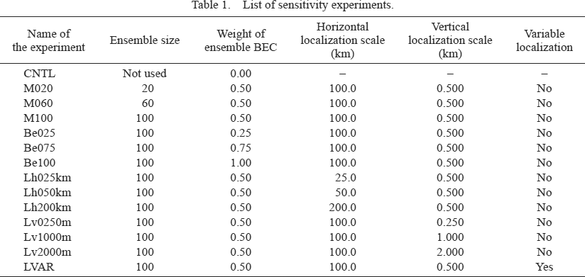
During the period of January 11–21 and July 2–15, 2020, sensitivity experiments assimilating real-data with the LA system (Figs. 1a–d and 10-hour forecasts with LFM) are conducted every 3 hours. The data assimilated in these experiments are the same as those in the operational LA system at the time of experiments and include surface (pressure, horizontal wind, temperature, and specific humidity), upper-air (horizontal wind, temperature, and relative humidity), radar (radial wind and relative humidity retrieved from reflectivity), and satellite (atmospheric motion vector, precipitable water vapor, brightness temperature, soil moisture) observations. These observations and the prescribed observation error variances for each type are summarized in Japan Meteorological Agency (2022). Here, the pure 3DVar experiment is called CNTL, and the hybrid 3DVar experiments with 20-, 60-, and 100-member ensemble forecasts (created by 6-hourly 1, 3, and 5 lagged forecasts of MEPS) are called M020, M060, and M100, respectively. In M020, 3–9-hour (3–6-hour or 6–9-hour) forecasts of MEPS (output hourly) are used in the four successive hybrid 3DVar (Figs. 1a–d). In M060, 9–15-hour and 15–21-hour forecasts are additionally used. In addition, 21–27-hour and 27–33-hour forecasts are also used in M100. The weights of hybrid BEC in M020, M060, and M100 are set as , while the e^−1/2-folding localization scales are set to 100 km horizontally and 0.5 km vertically. Moreover, other sensitivity experiments are also conducted to investigate the impacts of the weights of hybrid BEC (Be025, Be075, and Be100), horizontal localization scale (Lh025km, Lh050km, and Lh200km), vertical localization scale (Lv0250m, Lv1000m, and Lv2000m), and variable localization to cut off the cross-variable covariance (LVAR). Note that M020, M060, and M100 use manually tuned parameters based on the results of these sensitivity experiments shown in Section 5. The concrete settings of these experiments are shown in Table 1.

It should be noted that several heavy rain events occurred during the period of these experiments. This study focuses on the heavy rain event of July 3 that flooded large rivers in Kyushu Island (Hirockawa et al. 2020). In Radar/Raingauge-Analyzed Precipitation by JMA, the maximum 3-hour precipitation of over 300 mm was analyzed in 18–21 UTC on July 3. This heavy rain event was associated with the convergence of low-level warm and humid air at the upwind area of the rain along the Baiu front (a synoptic-scale stationary front that frequently emerge in the early summer in Japan). The impact of hybrid 3DVar in this event is examined in Section 5.

4. Results

4.1 Analysis increment in single-observation experiments

Figure 5 shows the analysis increment in each single-observation experiment assimilating the x-component of horizontal wind. In pure 3DVar (Fig. 5b), horizontal wind exhibited isotropic Gaussian-shaped analysis increment in x- and y-directions, while other variables, including sea level pressure, exhibited zero analysis increments, in accordance with the imposed structure of the static BEC. In contrast, in pure En3DVar (Figs. 5e, ff), all variables exhibited flow-dependent and nonzero analysis increments. However, variables other than the horizontal wind exhibited zero analysis increment even in En3DVar (not shown) when variable localization was applied (Appendix). In hybrid 3DVar (Figs. 5c, d), the analysis increment was close to the mean of the analysis increments of pure 3DVar and pure En3DVar.

The analysis increment of horizontal wind in the 60-member pure En3DVar (Fig. 5f) is smoother and larger near the center of the typhoon than that in the 20-member pure En3DVar (Fig. 5e). In addition, the analysis increment of sea level pressure decreased near the typhoon in the 60-member pure En3DVar; this finding is consistent with our expectation that the horizontal wind assimilation should strengthen the typhoon intensity. This observation demonstrates the mitigation of sampling error of the ensemble-based BEC by the use of a larger ensemble; a similar feature is also observed in hybrid 3DVar (Figs. 5c, d).

4.2 Statistical verification in real-data assimilation experiments

Figure 6 shows the statistical significance of score differences of the M020, M060, and M100 experiments in comparison to the CNTL experiment. The scores examined are the equitable threat scores (ETS) for 1-hour precipitation with several different thresholds and the root mean square errors (RMSE) of several forecast fields. The forecast range extends up to 10-hour, and the statistics are taken for the period of July 2–15. The reference data is JMA Radar/Raingauge-Analyzed Precipitation (R/A; Nagata 2011) for ETS and 12-hourly radiosonde and hourly surface observations in the calculation domain of the experiments for RMSE. As shown in the figure, M020, M060, and M100 showed better ETS of precipitation than CNTL, except for the small thresholds up to 2-hour forecast. This improvement was particularly evident for the threshold of 10–20 mm h⁻¹. Surface variables (pressure, temperature, wind speed, and specific humidity) in M020, M060, and M100 also showed better RMSE scores except for specific humidity in M020. However, the improvements in the RMSEs of upper-air variables were not judged statistically significant. This could be because the sample size for the upper-air verifications is limited due to the scarcity of radiosonde observations that are only available at 12-hourly intervals in comparison to the abundant surface observations (Fig. 7) that are available at hourly intervals.

Fig. 5

(a) First guess and (b–f) analysis increment of x-component of horizontal wind (color, m s⁻¹) and sea level pressure [contour, (a) 4 hPa and (b–f) 0.01 hPa intervals] in single-observation experiments [(b) pure 3DVar, (c) 20-member hybrid 3DVar, (d) 60-member hybrid 3DVar, (e) 20-member pure En3DVar, and (f) 60-member pure En3DVar].

Fig. 6

Scorecards of the ETS of precipitation in each threshold verified against R/A and the RMSE verified against radiosonde and surface observations (Z500: geopotential height at 500 hPa, T300-925: temperature at 300–925 hPa, MIXING300-925: water vapor mixing ratio at 300–925 hPa, WIND300-925: wind speed at 300–925 hPa, PSEA: sea level pressure, T1.5m: temperature at 1.5-m AGL, QV1.5m: specific humidity at 1.5-m AGL, WINDS10m: wind speed at 10-m AGL, DSWB: surface downward shortwave radiation) in July 2–15, 2020 of (a) M020, (b) M060, and (c) M100. Each value is different from that in CNTL divided by half of a 95 % confidence interval and shown hourly up to 10-hour forecast (T+10). Blue and red mean improvement (larger ETS or smaller RMSE) and degradation (smaller ETS or larger RMSE), respectively, in comparison to CNTL. Smaller and larger squares indicate significance values of 1.0 and 3.0, respectively.

Fig. 7

The distribution of surface observations assimilated in the first 3DVar (09 UTC) for creating the analysis at 12 UTC on July 3, 2020, in CNTL (black plus sign: horizontal wind; blue multiplication sign: temperature; red circle: specific humidity).

The weighted root mean square errors (WRMSE, Duc and Saito 2018) is shown for several kinds of observations assimilated in each experiment (Fig. 8) to clarify the improvement in the first guess. The WRMSE is defined as

  

where d_kⁱ denotes the k-th component of d_i (first guess departure in the i-th analysis), denotes square root of the k-th component of R_i (diagonal observation error covariance matrix in the i-th analysis), denotes the total number of observations assimilated over the verification period, and N_t denotes the number of analyses. The initial cost function in each analysis is , so the WRMSE can be obtained from J i^Init and N_o by:

  

Fig. 8

WRMSE for all (black bars), upper-air wind (red lines), upper-air temperature (blue lines), surface wind (purple lines), and surface temperature (light blue lines) observations assimilated in all periods (January 11–21 and July 2–15, 2020) of each experiment. Each is normalized by WRMSE of CNTL to show the improvement against CNTL. Note that M100 = Be050 = Lh100km = Lv0500m = NLVAR.

The WRMSEs obtained in M020, M060, and M100 were smaller than that in CNTL, especially for surface temperature (Fig. 8). The WRMSEs for upper-air temperature in M060 and M100 were smaller than that in CNTL, while it was larger in M020. Thus, a larger ensemble size resulted in a smaller WRMSE.

The larger improvement of surface variables with the increase in ensemble size was evident up to at least 10 hours, especially for surface temperature (Figs. 9a, b) and surface specific humidity (Figs. 10a, b). At the initial time, the RMSE of surface temperature in hybrid 3DVar, especially in M100, was smaller than that in CNTL. This tendency was observed up to at least 10 hours, implying that the analysis increment of surface temperature in hybrid 3DVar was larger and resulted in the analysis that is more natural as the initial condition for the forecast. Unlike the surface temperature scores, the RMSE of surface specific humidity at the initial time was larger in hybrid 3DVar than in CNTL. Nevertheless, this RMSE value decreased quickly within an hour, except in M020 that showed larger RMSE presumably due to the scarcity of surface specific humidity observations in comparison to surface temperature observations (Fig. 7). As mentioned previously, the cross-variable covariance with temperature affects the analysis increment in specific humidity in hybrid 3DVar. Thus, a large difference between the analysis and the observation of surface specific humidity is an expected outcome due to the sampling error of this cross-variable covariance when assimilating many surface temperature observations (Fig. 7) with the small ensemble size. Here, the number of total surface observations is O (10²) within a radius of the horizontal localization scale (100 km) and larger than the ensemble size in M020. In fact, this degradation was not observed in the experiment with the large ensemble size (M060 and M100).

Fig. 9

RMSE of temperature at 1.5-m AGL against surface observations (K) in July 2–15, 2020 of CNTL, M100, M060, and M020 and (b-f) the difference from that of CNTL [(b) M100-020, (c) Be025-100, (d) Lh025-200km, (e) Lv0250-2000m, (f) LVAR and NLVAR] in each forecast time (h). The error bar indicates a 95 % confidence interval estimated with the bootstrap method (1000 samples). Note that M100 = Be050 = Lh100km = Lv0500m = NLVAR.

Fig. 10

As in Fig. 9, but the RMSE of specific humidity at 1.5-m AGL verified against surface observations (g kg⁻¹).

Compared to CNTL, the ETS of precipitation was also better in hybrid 3DVar, especially in M060 and M100 (Figs. 11a, b). The ETS was not improved for small thresholds up to 2-hour forecasts (Fig. 6), but the ETS for the threshold of 10–20 mm h⁻¹ was clearly improved. This improvement could be attributed to the improvement in the analysis of surface wind and temperature, which is discussed in the next section. Figures 9–11 demonstrate the forecast improvements by hybrid 3DVar during the period of July 2–15, 2020, but such improvements are not limited to the heavy rainfall in summer because similar forecast improvements were also observed for the winter period of January 11–21, 2020 (not shown).

Fig. 11

As in Fig. 9, but the ETS of precipitation at each threshold verified against R/A (mm h⁻¹).

5. Discussion

5.1 Impact on the heavy rain event on July 3, 2020

The forecast initialized at 12 UTC on July 3, 2020 in each sensitivity experiment predicted occurrence of heavy rain in Kyushu Island in 18–21 UTC on the same day. The predicted heavy rain was positioned closer to the observations (Fig. 12f) in hybrid 3DVar experiments (Figs. 12b–d) than in CNTL (Fig. 12a). The predicted heavy rain was the closest in M100 compared to M020 and M060. In particular, 3-hour accumulated precipitation for 18–21 UTC in M100 exceeded 100 mm over the land, which is consistent with the observation.

Fig. 12

Forecasts of 3-hour accumulated precipitation amount (mm) in (a) CNTL, (b) M020, (c) M060, (d) M100, and (e) Be100 (initial time: 12 UTC on July 3, 2020) and (f) Radar/Raingauge-Analyzed Precipitation for 18–21 UTC on July 3, 2020. Blue contours indicate Radar/Raingauge-Analyzed Precipitation of 100 mm.

The flow-dependent analysis increment in hybrid 3DVar improved the position of the predicted heavy rain. Figure 13 shows the analysis increment and the first guess in the first of four (hybrid) 3DVar analyses (Fig. 1a) that was run to produce the initial state of the forecast initialized at 12 UTC. In this first guess validating at 09 UTC, the Baiu front was predicted approximately along 32°N, as identified as the convergence of horizontal wind and steep horizontal temperature gradient near the sea surface (Fig. 13f). In this area over the sea, upwind of the heavy rain, the analysis increment was large in hybrid 3DVar (Figs. 13b–d), while it was almost zero in pure 3DVar (Fig. 13a). This is because the horizontal correlation scale of the climatological BEC (Fig. 3) is smaller than the horizontal localization scale of the ensemble-based BEC (100 km) near the surface. Although not observed in M020, the analysis increment in hybrid 3DVar raised surface temperature and strengthened the near-surface convergence near the upwind area of the heavy rain in M060 and M100. In addition, the resulting heavy rain was positioned nearer to the observation in M100 than in M060 probably because of the stronger southerly wind at the south of the convergence (Fig. 13d).

Fig. 13

Analysis increments of temperature at 1.5-m AGL (color, K) and horizontal wind at 10-m AGL (arrows, m s⁻¹) in first (hybrid) 3DVar (09 UTC) for creating the analysis at 12 UTC on July 3, 2020, in (a) CNTL, (b) M020, (c) M060, (d) M100, and (e) Be100 and (f) the common first guess of these analyses.

The analysis increments in M020, M060, and M100 differed because of the difference in the ensemble-based BEC component that resulted from the use of different lagged ensemble forecasts. Figure 14 shows the ensemble standard deviations of surface wind and temperature used for ensemble-based BECs in M020, M060, and M100. The ensemble spread in M020 was based on 3-hour ensemble forecasts in MEPS, in which the forecast range was too short to allow the ensemble spread to sufficiently grow. This is because the optimization time interval of SVs in MEPS is longer than 3 hours. Thus, the ensemble spread was large only near the Baiu front in M020 (Figs. 14a, d, g). By contrast, the ensemble spread in M060 (Figs. 14b, e, h) and M100 (Figs. 14c, f, i) exhibited smoother and larger distribution, especially around the upwind area of the heavy rain. This indicates the advantage of using lagged ensemble forecasts. If the error of the first guess can be represented precisely by ensemble forecasts from a single initial time, the ensemble-based BEC with more members created by lagged ensemble forecasts may not be necessarily better due to the inclusion of older data. However, this disadvantage was not clearly evident here, presumably because the SV-based ensemble forecasts in MEPS do not depend on LA and thus are not directly linked to the error of the first guess.

Fig. 14

Ensemble standard deviations of (a–c) x-component of horizontal wind at 10-m AGL (m s⁻¹), (d–f) y-component of horizontal wind at 10-m AGL (m s⁻¹), (g–i) temperature at 1.5-m AGL (K) used in first (hybrid) 3DVar (09 UTC) for creating the analysis at 12 UTC on July 3, 2020, in (a, d, g) M020, (b, e, h) M060, and (c, f, i) M100.

5.2 Sensitivity to the weights of ensemble-based background error covariance

The weights of adopted in M020, M060, and M100 may not be necessarily optimal for all variables. In fact, Be025 resulted in the smallest WRMSE for upper-air temperature, and likewise for Be050 (= M100) for surface temperature and upper-air wind, and Be100 for surface wind (Fig. 8). The RMSEs of surface variables at the analysis time were smaller in experiments with smaller β_e (Figs. 9c, 10c) because horizontally-averaged ensemble-based background error standard deviations are smaller than the climatological one near the surface (Fig. 4). However, the forecasts showed that these RMSEs of surface variables were the smallest in Be050. This implies that the use of purely climatological homogeneous BEC, or purely ensemble-based BEC that may include large sampling errors, does not lead to a better analysis. Instead, the use of hybrid BEC contributed to better analysis partly because a smaller weight given to the ensemble-based BEC can dilute sampling errors even without making the localization scales smaller.

As for precipitation forecast, smaller β_e degraded the ETS for strong precipitation (Fig. 11c) probably because of the smaller climatological BEC at the upwind area of the precipitation. In comparison, larger β_e degraded the ETS for weak precipitation (Fig. 11c) probably because of the smaller ensemble-based BEC in the region where the precipitation is not predicted. The location of the predicted heavy rain on July 3 in Be100 (Fig. 12e) was closer to the observations than that in Be050 (Fig. 12d). This could be because of the larger ensemble-based BEC and associated larger analysis increments at the upwind area of the heavy rain (Figs. 13d, e).

5.3 Sensitivity to the localization scale and the variable localization

The e^−1/2-folding scales of horizontal and vertical localizations in M020, M060, and M100 were set to 100 km and 0.5 km, respectively, and variable localization was not applied. Measuring with WRMSE (Fig. 8), the horizontal localization scale of 100 km (Lh100km) was best for upper-air wind and surface temperature, while a horizontal localization scale of 200 km (Lh200km) was better for upper-air temperature and surface wind. As for vertical localization, a larger scale than 0.5 km (Lv1000m and Lv2000m) was better for winds and surface temperature, while a smaller one (Lv0250m) was better for upper-air temperature. These differences could be due to the different spatial representativeness of each variable. In addition, variable localization (LVAR) was found to be beneficial for the WRMSE of surface variables but not for upper-air variables. This indicates the importance of cross-variable correlation of upper-air variables.

The use of a smaller localization scale or variable localization reduced the RMSE at the initial time of the forecast (Figs. 9d–f, 10d–f) because the analysis increment was created by a smaller number of observations near each analysis point, including the reference observations used in calculating the RMSE. However, experiments with such “strong” localizations exhibited larger RMSE of the long-term forecasts, except for surface specific humidity that is not directly related to dynamical balance (Fig. 10f). This indicates the localization scale should be large to some extent, without the variable localization, so as to prevent the collapse of the dynamical balance.

The experiment with the horizontal localization scale of 100 km showed the largest ETS of precipitation. The use of a smaller scale (Lh025km and Lh-050km) reduced the ETS of precipitation, especially for strong precipitation exceeding 5 mm h⁻¹, while the use of a larger scale (Lh200km) reduced the ETS of precipitation, especially for weak precipitation below 5 mm h⁻¹ (Fig. 11d). This indicates that the large analysis increment associated with “strong” localization is beneficial for forecast of weak precipitation, but the resulting dynamical imbalance can be harmful for forecast of strong precipitation. On the other hand, the experiments with smaller vertical localization scales (Lv0250m) or variable localization (LVAR) showed even worse ETS, especially for strong precipitation (Figs. 11e, f). This implies that the vertical correlation and the cross-variable correlation are large in the region of the deep convection and have large impacts on the forecast of strong precipitation associated with the convection.

The impacts of localization indicated above are manifested in a more concrete manner with the precipitation forecasts of the heavy rain on July 3. In this case, both the smaller and larger horizontal localization scale (Lh025km and Lh200km, respectively) shifted the position of the predicted heavy rain south-westward (Figs. 15a, b) because both the narrower and wider analysis increments resulted in lower surface temperature and weaker horizontal convergence at the upwind area of the heavy rain (Figs. 16a, b). The precipitation forecasts were worse also in LVAR (Fig. 15e) because lower surface temperature at the upwind area was caused by the variable localization due to cutting off of the cross-variable correlation (Fig. 16e). In comparison, changing the vertical localization scale (Lv0250m and Lv2000m) hardly affected the horizontal distributions of surface analysis increments (Figs. 16c, d). However, the experiments with smaller (larger) vertical localization scale exhibited vertically finer (smoother) analysis increments (not shown), which probably increased (decreased) spurious convections due to the dynamical imbalance and resulted in worse (better) precipitation forecasts (Fig. 15c, d).

Fig. 15

As in Figs. 12a–e but for (a) Lh025km, (b) Lh200km, (c) Lv0250m, (d) Lv2000m, and (e) LVAR.

Fig. 16

As in Figs. 13a–e but for (a) Lh025km, (b) Lh200km, (c) Lv0250m, (d) Lv2000m, and (e) LVAR.

6. Conclusions

This study examined the impact of introducing hybrid covariance to the hourly 3DVar by implementing a hybrid formulation to the operational LA with MEPS. This hybrid 3DVar uses the weighted average of the climatological and ensemble-based BECs. The covariance inflation, which makes the ensemble variances of forecasts with different lead times comparable to that of the climatological BEC, is introduced here to mitigate the difference in ensemble spreads between each forecast time (Fig. 4). In particular, this study focused on (i) the difference between pure and hybrid 3DVar, (ii) the impact of increasing ensemble size with 6-hourly lagged ensemble forecasts in MEPS, and (iii) the sensitivities to the weight of ensemble-based BECs, to the horizontal and vertical localization scales, and to the cross-variable correlation. To our knowledge, this is the first study to clarify the impact of hybrid 3DVar with time-lagged SV-based ensemble forecasts.

Single virtual observation assimilation experiments and real-data assimilation experiments showed that increasing the ensemble size with lagged ensemble forecasts yields smoother analysis increments, more reasonable cross-variable correlation, and the associated improvement in forecast scores (Figs. 5, 6, 8–11). The experiments with hybrid 3DVar, especially with a larger ensemble size, showed better ETS for strong precipitation and better RMSE of surface variables than those with pure 3DVar. These results indicate that SV-based ensemble forecasts, even without ensemble data assimilation-based perturbations, and increased ensemble size with lagged ensemble forecasts, can improve the BEC and the associated hybrid 3DVar analysis.

In the heavy rain case of July 3, 2020, the experiments of hybrid 3DVar with a larger ensemble size positioned the predicted heavy rain closer to the observation (Fig. 12). This improvement was due to the flow-dependent analysis increment, which yielded warmer surface temperature and stronger surface convergence at the upwind area of the heavy rain along the Baiu front (Fig. 13). This larger analysis increment was associated with the smoother and larger ensemble spread around the Baiu front in the BEC created by the larger number of lagged ensemble forecasts (Fig. 14). However, the application of the larger weight to the ensemble-based BEC and the larger localization scale did not necessarily improve the forecasts partly because of the smaller analysis increments that result from large sampling errors. In the hybrid 3DVar of this study, the optimal weight for the ensemble-based BEC and the optimal horizontal localization scale were found to be about 0.5 and 100 km, respectively. Smaller weights given to the ensemble-based BEC, smaller vertical localization scales, or a use of variable localization did not improve the rainfall forecasts likely because that resulted in analysis increments being less dynamically balanced, which indicates that the large-scale vertical correlation and the cross-variable correlation are important for heavy rain forecasts.

In March 2022, JMA implemented the hybrid 3DVar with the setting of M100 in the operational LA system (Yokota et al. 2022). By utilizing the operational SV-based MEPS for the creation of flow-dependent BECs, JMA realized hourly hybrid 3DVar, which can improve the accuracy of forecasting heavy rainfall, without requiring an ensemble data assimilation system. This is a strategy to achieve a data assimilation system that improves forecast accuracy with currently available computational resources. However, the weight given to the ensemble-based BEC (0.5) and the localization scales (100 km horizontally and 0.5 km vertically) are not necessarily optimal at all times. These settings may be improved by using the recently suggested optimization methods (e.g., Ménétrier and Auligné 2015) and scale-dependent localization (Buehner 2012; Buehner and Shlyaeva 2015).

If more computer resources become available in the future, operating a regional ensemble data assimilation system should also be considered because the error of the first guess is not always precisely represented by ensemble forecasts without data assimilation. On the other hand, improvements that do not require a significant increase in computing resources are also required. In any case, it is essential to make the ensemble forecasts represent the error of the first guess within the tight computational time limit.

Data Availability Statement

Some of the datasets and program codes used in this study are not publicly available due to the management policy of Japan Meteorological Agency, but may be available from the relevant authors for reasonable usage upon request. All rights reserved with JMA.

Acknowledgments

The authors thank colleagues in the Numerical Prediction Development Center at JMA for the cooperation in implementing hybrid 3DVar on the LA system and Dr. Takuya Kawabata in the Meteorological Research Institute at JMA, the editor Dr. Daisuke Hotta, and two anonymous reviewers for many thoughtful comments. This work was supported in part by Japan Society for the Promotion of Science KAKENHI Grant Number JP21K03671. The authors would like to thank Enago (https://www.enago.jp) for the English language review.

Appendix: Implementation of horizontal, vertical, and variable localizations

In this study, the N × N localization matrix C in the hybrid 3DVar is defined as

  

where “⨂” denotes Kronecker product, C_X and C_Y denote n_x × n_x and n_y × n_y matrices for x- and y-direction horizontal localization, respectively [n_x(y): the number of horizontal grids in x(y)-direction], and C_V denotes n_v × n_v matrix for vertical and variable localization (n_v : the sum of the number of vertical grids of all variables). According to Eq. (A1), the square root of C is written as (N × L matrix, where N = n_xn_yn_v and L is the rank of C).

is the 1-dimensional recursive filter (Purser et al. 2003). Note that the e^−1/2 scale of is if the e^−1/2 scale of C_X(Y) is set to σ_x(y). On the other hand, the eigenvalue decomposition of C_z is used to obtain because, with the small number of vertical levels, square-root representation with eigenvalue decomposition is computationally feasible. Here, C_z is composed of Gaussian functions of the vertical distance from the height of each vertical level (Fig. A1). Since the height for surface pressure, soil temperature, and soil moisture is regarded as 0-m AGL, which is lower than the lowest level of atmosphere, and the vertical distance in underground is neglected, C_z is the (n_z + 1) × (n_z + 1) matrix (n_z : the number of vertical layers of atmosphere). The square root of C_z is written as , where Λ denotes a diagonal matrix composed of eigenvalues of C_z, and V denotes an orthogonal matrix composed of eigenvectors of C_z. If i-th member ensemble perturbation at a given horizontal grid point is written as

  

the corresponding , which does not apply variable localization to, is

  

where , and denote n_xn_yn_z-dimension vectors of ensemble perturbations of x-component of horizontal wind, y-component of horizontal wind, potential temperature, and pseudo relative humidity, respectively. denotes n_xn_yn_t-dimension vector of soil temperature (n_t: the number of vertical layers of soil temperature), denotes n_xn_yn_w-dimension vector of soil moisture (n_w: the number of vertical layers of soil moisture), denotes n_xn_y-dimension vector of surface pressure, denotes matrix that is composed of only a row for the lowest level of denotes matrix omitting from , and denotes matrix that is composed of n copies of . Therefore, this is matrix, and the resultant rank of is L = n_xn_y(n_z + 1). When using Eq. (A3), C_V is written as

  

where , and .

In addition, the variable localization is implemented when in Eq. (A3) is replaced by

  

Fig. A1

Structure of vertical localization matrix (e^−1/2-folding scale: 0.5 km).

When using Eq. (A5), the number of control variables, which is proportional to L, becomes fourfold compared to using Eq. (A3), and the cross-variable correlations are ignored as

  

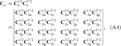
Note that Eq. (A6) is the same as Eq. (A4) except for the localization for the cross-variable covariances.

References

•  Andersson,  E., and  H.  Järvinen, 1999: Variational quality control. Quart. J. Roy. Meteor. Soc., 125, 697–722.
•  Benjamin,  S. G.,  S. S.  Weygandt,  J. M.  Brown,  M.  Hu,  C. R.  Alexander,  T. G.  Smirnova,  J. B.  Olson,  E. P.  James,  D. C.  Dowell,  G. A.  Grell,  H.  Lin,  S. E.  Peckham,  T. L.  Smith,  W. R.  Moninger,  J. S.  Kenyon, and  G. S.  Manikin, 2016: A North American hourly assimilation and model forecast cycle: The rapid refresh. Mon. Wea. Rev., 144, 1669–1694.
•  Buehner,  M., 2012: Evaluation of a spatial/spectral covariance localization approach for atmospheric data assimilation. Mon. Wea. Rev., 140, 617–636.
•  Buehner,  M., and  A.  Shlyaeva, 2015: Scale-dependent background-error covariance localisation. Tellus A, 67, 28027.
•  Buehner,  M.,  J.  Morneau, and  C.  Charette, 2013: Four-dimensional ensemble-variational data assimilation for global deterministic weather prediction. Nonlinear Processes Geophys., 20, 669–682.
•  Cameron,  J., and  W.  Bell, 2018: The testing and implementation of variational bias correction (VarBC) in the Met Office global NWP system. Wea. Sci. Tech. Report, 631, 1–22.
•  Clayton,  A. M.,  A. C.  Lorenc, and  D. M.  Barker, 2013: Operational implementation of a hybrid ensemble/4D-Var global data assimilation system at the Met Office. Quart. J. Roy. Meteor. Soc., 139, 1445–1461.
•  Dee,  D. P., and  A. M.  da Silva, 2003: The choice of variable for atmospheric moisture analysis. Mon. Wea. Rev., 131, 155–171.
•  Dowell,  D. C.,  C. R.  Alexander,  E. P.  James,  S. S.  Weygandt,  S. G.  Benjamin,  G. S.  Manikin,  B. T.  Blake,  J. M.  Brown,  J. B.  Olson,  M.  Hu,  T. G.  Smirnova,  T.  Ladwig,  J. S.  Kenyon,  R.  Ahmadov,  D. D.  Turner,  J. D.  Duda, and  T. I.  Alcott, 2022: The High-Resolution Rapid Refresh (HRRR): An hourly updating convection-allowing forecast model. Part I: Motivation and system description. Wea. Forecasting, 37, 1371–1395.
•  Duc,  L., and  K.  Saito 2018: Verification in the presence of observation errors: Bayesian point of view. Quart. J. Roy. Meteor. Soc., 144, 1063–1090.
•  Ehrendorfer,  M.,  R. M.  Errico, and  K. D.  Raeder, 1999: Singular-vector perturbation growth in a primitive equation model with moist physics. J. Atmos. Sci., 56, 1627–1648.
•  Evensen,  G., 1994: Sequential data assimilation with a nonlinear quasi-geostrophic model using Monte Carlo methods to forecast error statistics. J. Geophys. Res., 99, 10143–10162.
•  Hacker,  J. P.,  J. L.  Anderson, and  M.  Pagowski, 2007: Improved vertical covariance estimates for ensemblefilter assimilation of near-surface observations. Mon. Wea. Rev., 135, 1021–1036.
•  Hamill,  T. M., and  C.  Snyder, 2000: A hybrid ensemble Kalman filter-3D variational analysis scheme. Mon. Wea. Rev., 128, 2905–2919.
•  Hamill,  T. M.,  J. S.  Whitaker, and  C.  Snyder, 2001: Distance-dependent filtering of background error covariance estimates in an ensemble Kalman filter. Mon. Wea. Rev., 129, 2776–2790.
•  Hirockawa,  Y.,  T.  Kato,  K.  Araki, and  W.  Mashiko, 2020: Characteristics of an extreme rainfall event in Kyushu district, southwestern Japan in early July 2020. SOLA, 16, 265–270.
•  Houtekamer,  P. L., and  H. L.  Mitchell, 2001: A sequential ensemble Kalman filter for atmospheric data assimilation. Mon. Wea. Rev., 129, 123–137.
•  Ikuta,  Y.,  T.  Fujita,  Y.  Ota, and  Y.  Honda, 2021: Variational data assimilation system for operational regional models at Japan Meteorological Agency. J. Meteor. Soc. Japan, 99, 1563–1592.
•  Isaksen,  L.,  M.  Bonavita,  R.  Buizza,  M.  Fisher,  J.  Haseler,  M.  Leutbecher, and  L.  Raynaud, 2010: Ensemble of data assimilations at ECMWF. ECMWF Tech. Memorandum, 636, 48 pp.
•  Ishibashi,  T., 2015: Tensor formulation of ensemble-based background error covariance matrix factorization. Mon. Wea. Rev., 143, 4963–4973.
•  Japan Meteorological  Agency, 2022: Outline of the operational numerical weather prediction at the Japan Meteorological Agency. Appendix to WMO Technical Progress Report on the Global Data-processing and Forecasting System (GDPFS) and Numerical Weather Prediction (NWP) Research. 246 pp. [Available at https://www.jma.go.jp/jma/jma-eng/jma-center/nwp/outline2022-nwp/index.htm.]
•  Kim,  O.-Y.,  C.  Lu,  J. A.  McGinley,  S. C.  Albers, and  J.-H.  Oh, 2013: Experiments of LAPS wind and temperature analysis with background error statistics obtained using ensemble methods. Atmos. Res., 122, 250–269.
•  Kleist,  D. T., and  K.  Ide, 2015: An OSSE-based evaluation of hybrid variational-ensemble data assimilation for the NCEP GFS. Part I: System description and 3D-Hybrid results. Mon. Wea. Rev., 143, 433–451.
•  Lei,  L., and  J. L.  Anderson, 2014: Empirical localization of observations for serial ensemble Kalman filter data assimilation in an atmospheric general circulation model. Mon. Wea. Rev., 142, 1835–1851.
•  Liu,  C.,  Q.  Xiao, and  B.  Wang, 2009: An ensemble-based four-dimensional variational data assimilation scheme. Part II: Observing system simulation experiments with Advanced Research WRF (ARW). Mon. Wea. Rev., 137, 1687–1704.
•  Lorenc,  A. C., 2003: The potential of the ensemble Kalman filter for NWP—a comparison with 4D-Var. Quart. J. Roy. Meteor. Soc., 129, 3183–3203.
•  Ménétrier,  B., and  T.  Auligné 2015: Optimized localization and hybridization to filter ensemble-based covariances. Mon. Wea. Rev., 143, 3931–3947.
•  Nagata,  K., 2011: Quantitative precipitation estimation and quantitative precipitation forecasting by the Japan Meteorological Agency. Technical Review No. 13 of RSMC Tokyo, RSMC Tokyo - Typhoon Center, 37–50. [Available at https://www.jma.go.jp/jma/jma-eng/jma-center/rsmc-hp-pub-eg/techrev/text13-2.pdf.]
•  Ono,  K., 2020: Extension of the Lanczos algorithm for simultaneous computation of multiple targeted singular vector sets. Quart. J. Roy. Meteor. Soc., 146, 454–467.
•  Ono,  K.,  M.  Kunii, and  Y.  Honda, 2021: The regional modelbased Mesoscale Ensemble Prediction System, MEPS, at the Japan Meteorological Agency. Quart. J. Roy. Meteor. Soc., 147, 465–484.
•  Parrish,  D. F., and  J. C.  Derber, 1992: The National Meteorological Center’s spectral statistical-interpolation analysis system. Mon. Wea. Rev., 120, 1747–1763.
•  Purser,  R. J.,  W. S.  Wu,  D. F.  Parrish, and  N. M.  Roberts, 2003: Numerical aspects of the application of recursive filters to variational statistical analysis. Part I: Spatially homogeneous and isotropic Gaussian covariances. Mon. Wea. Rev., 131, 1524–1535.
•  Sasaki,  Y., 1958: An objective analysis based on the variational method. J. Meteor. Soc. Japan, 36, 77–88.
•  Sasaki,  Y., 1969: Proposed inclusion of time variation terms, observational and theoretical, in numerical variational objective analysis. J. Meteor. Soc. Japan, 47, 115–124.
•  Talagrand,  O., and  P.  Courtier, 1987: Variational assimilation of meteorological observations with the adjoint vorticity equation. I: Theory. Quart. J. Roy. Meteor. Soc., 113, 1311–1328.
•  Thompson,  P. D., 1969: Reduction of analysis error through constraints of dynamical consistency. J. Appl. Meteor. Climatol., 8, 738–742.
•  Wang,  Y.,  J.  Min,  Y.  Chen,  X.-Y.  Huang,  M.  Zeng, and  X.  Li, 2017: Improving precipitation forecast with hybrid 3DVar and time-lagged ensembles in a heavy rainfall event. Atmos. Res., 183, 1–16.
•  Yamaguchi,  M.,  R.  Sakai,  M.  Kyoda,  T.  Komori, and  T.  Kadowaki, 2009: Typhoon ensemble prediction system developed at the Japan Meteorological Agency. Mon. Wea. Rev., 137, 2592–2604.
•  Yokota,  S.,  T.  Banno,  M.  Oigawa,  G.  Akimoto,  K.  Kawano, and  Y.  Ikuta, 2022: Implementation of hybrid 3DVar in JMA’s local analysis. CAS/JSC WGNE Res. Activ. Activ. Earth Syst. Modell., 52, 01.19–01.20. [Available at https://wgne.net/bluebook/uploads/2022/docs/01_YOKOTA_Sho_Hybrid3DVar.pdf.]