Article
Short-Term Predictability of Extreme Rainfall Using Dual-Polarization Radar Measurements

2024 Volume 102 Issue 2 Pages 151-165

Details
2024 Volume 102 Issue 2 Pages 151-165
Dual-polarization radar often detects columnar regions of enhanced differential reflectivity (ZDR) extending vertically above the environmental 0 °C level. Indicative of supercooled liquid drops and wet ice particles lofted by strong updrafts, these ZDR columns are increasingly understood to be of use in predicting extreme rainfall. With the aim of achieving practical application of ZDR column measurements, this paper focuses on the relationship between the height of ZDR columns and rainfall intensity near the ground.
All the data on ZDR columns analyzed in this study was collected from weather radar stations in Japan. The height of each column and rainfall rates at low levels were analyzed using an automated algorithm. A regression analysis result reveals peak column height to be positively correlated with maximum rainfall rate near ground level, and that rainfall intensity on the ground is likely to exceed 50 mm h−1 when radar identifies a ZDR column. Furthermore, extreme rainfall with an intensity of 180 mm h−1 or more is likely associated with a column over 3 km tall from the 0 °C level. These findings suggest that surveillance of ZDR columns can contribute to the reliability of very short-range forecasts or nowcasts as well as assist with the issue of early warnings of extreme rainfall and flash floods.
Increasing global warming has resulted in greater frequency and intensity of extreme precipitation events around the world, caused by increased evaporation and atmospheric water-holding capacity attributed to higher temperatures, as governed by the Clausius-Clapeyron (CC) relation (e.g., Min et al. 2011; Seneviratne et al. 2021). Numerous studies have been carried out on the association between atmospheric temperature and heavy precipitation, some of which demonstrate that the frequency of short-duration extremes may even exceed predictions based on the CC rate (e.g., Lenderink and Van Meijgaard 2008) and that the intensity of sub-daily extremes increases more rapidly than that of daily-scale events (e.g., Westra et al. 2014).
In recent decades, heavy precipitation events have often impacted human society and the environment, mainly through rain-triggered disasters such as floods, the most common natural hazard worldwide. Across the 2001–2020 period, an average of 357 annual catastrophic events were recorded, in which floods (163) predominated (Centre for Research on the Epidemiology of Disasters 2022b). In 2022, India and Pakistan experienced devastating floods after extreme rainfall, each with more than one thousand deaths (Centre for Research on the Epidemiology of Disasters 2022a). Flood risks such as these are predicted to increase with the acceleration of urbanization, due to the expansion of impervious surfaces and subsequent loss of infiltration capacity (e.g., Tingsanchali 2012).
The major damage that is often caused by extreme rainfall is prompting research on enhancing the resolution of operational numerical weather prediction models to provide more realistic forecasts of local weather, especially of precipitation. Despite the increasing accuracy of rainfall forecasts, an element of uncertainty remains in all models. A large proportion of this uncertainty derives from assumptions made in the parameterization of unresolved cloud micro-physical processes. However, a certain amount of information can be gained from dual-polarization radar observations (e.g., Roberts and Lean 2008; Seifert 2011; Adachi et al. 2015; Trömel et al. 2021).
The National Weather Service (NWS) completed the dual-polarization upgrade of its Weather Service radar (WSR-88D) in 2013 (Gerard 2021), and the Japan Meteorological Agency (JMA) started upgrading its operational weather radar in March 2020 (Japan Meteorological Agency 2022). Sending and receiving signals with both horizontal and vertical polarization, dual-polarization radar, or polarimetric radar can provide beneficial polarimetric variables that deliver information concerning hydrometeor size, shape, and orientation by comparing the amplitudes and phases of the signals returned at both polarizations. Of these variables, the differential reflectivity, or ZDR, is a function of the shapes of hydrometeors. Higher values of ZDR are recorded when raindrops grow and take on a more oblate spheroidal shape.
Polarimetric radar observations of deep convective clouds frequently show upward extensions of positive ZDR above the environmental 0 °C level where ice particles are usually distributed. These signatures, known as ZDR columns, contain supercooled liquid drops lofted by strong updrafts (Kumjian 2013b). Recent studies have shown that ZDR column evolution is linked to convective cloud development. For example, Kumjian et al. (2012) clarified the correlation between ZDR column height and updraft intensity using a simplified theoretical model, and Adachi et al. (2013) presented a method of detecting potentially hazardous convective clouds that produce extreme rainfall by identifying ZDR columns. Picca et al. (2010) and Kumjian et al. (2014) describe how growth in the horizontal and vertical directions of ZDR columns precedes, by 10–30 minutes, an increase in low-level radar reflectivity. Snyder et al. (2015) proposed an automated ZDR column algorithm designed to monitor the changes in ZDR column height and provide near-real-time information on the intensity and location of updrafts. Kuster et al. (2020) state that ZDR columns can be used to arrive at specific warning decisions for convective storms.
Despite these findings, the relationship between ZDR column height and rainfall intensity produced by the convective cloud has hitherto not been quantitatively evaluated. This prompted us to investigate the relationship between peak ZDR column height and momentary maximum rainfall rate near ground level using regression analysis of the rapid-update radar data observed in the Tokyo metropolitan area with a view to the more general application of ZDR column information to short-term rainfall prediction.
This paper focuses on isolated ZDR columns producing localized heavy rainfall for ease of analysis and looks at those measured by the dual-polarization Doppler weather radar at Haneda airport (Haneda radar) on 11 July 2021. The next section describes the instrumentation and analytical data. Section 3 covers data analysis techniques using dual-polarization radar measurements. Section 4 provides the analysis results of the relationship between ZDR column height and rainfall intensity near the ground, followed by our Discussion in Section 5. The paper closes with a brief conclusion in Section 6 that summarizes our findings.
Doppler Radar for Airport Weather (DRAW) has been installed at major airports in Japan to monitor weather conditions for the safe operation of aircraft. The data sources in this study are the Haneda radar for the most part, but also the Narita radar at Narita International Airport for 0 °C level estimation. Haneda and Narita airports both operate C-band dual-polarized radar that provides a suite of polarimetric variables including the reflectivity factors (ZH, ZV), differential reflectivity (ZDR), total differential phase shift (ΨDP), specific differential phase (KDP), and co-polar correlation coefficient (ρHV). Their data are collected up to a maximum range of 120 km with an azimuthal resolution of 0.7° and a radial resolution of 150 m. The volume scans are updated every five minutes and each scan comprises twelve plan-position indicator (PPI) scans at elevation angles of 0.7, 1.1, 1.5, 2.1, 2.8, 3.8, 5.1, 6.9, 9.2, 12.5, 17.0, and 90°. Five PPI scans at an elevation angle of 0.7° are included in each volume scan to improve the time resolution near the ground. The details of the Haneda radar are given in Table 1.

The Parsivel is a laser-based optical disdrometer for simultaneous measurement of PARticle SIze and VELocity of hydrometeors, designed by Löffler-Mang and Joss (2000) and formerly manufactured by PM Tech, but by OTT after 2004. In this study, we employed an OTT Parsivel (Version 1) disdrometer installed at the Kumagaya observation site.
The Parsivel is equipped with a laser sensor that produces a horizontal sheet of light measuring 30 mm × 180 mm, with a transmitter and receiver integrated into a single protective housing. Precipitation particles passing through the laser beam block a portion of the beam in proportion to their diameter, causing a reduction of the output voltage. The maximum attenuation of the signal is a measure of the particle size, and the time taken for the particle to pass through the laser beam allows an estimate of its velocity (e.g., Löffler-Mang and Joss 2000; OTT 2005).
The OTT Parsivel disdrometer can estimate particle sizes ranging from 0.2 mm to 25 mm in diameter and velocities from 0.2 m s−1 to 20 m s−1. After determining their diameters and velocities, it classifies them into one of 32 separate size and velocity classes with a high temporal resolution of one minute. It is therefore more suitable than a tipping bucket rain gauge for observations of heavy convective rainfall events of the type shown in this study (Section 4.1).
b. Surface observation networkThe Automated Meteorological Data Acquisition System (AMeDAS), an observation network of Automatic Weather Stations (AWSs) run by the JMA, measures precipitation, wind direction and speed, temperature, and humidity to support real-time monitoring of weather conditions. The JMA currently operates about 1,300 rain gauges at average intervals of 17 km nationwide. Each gauge records the amount of precipitation in units of 0.5 mm with a temporal resolution of ten minutes (Japan Meteorological Agency 2021). In this study, precipitation data obtained from the Kumagaya observation site is used for accuracy verification of rainfall rates from the co-located disdrometer.
2.3 Case informationThe data analyzed in this study were collected using the abovementioned instruments from 13:00 JST (Japan Standard Time: JST = UTC + 9 h) to 18:00 JST on 11 July 2021. On that day, dozens of ZDR columns were observed by the Haneda radar, and the atmospheric condition was unstable due to a stationary front, resulting in heavy precipitation over the Kanto region (eastern Japan). Figure 1 shows the distribution of the rainfall estimates and the locations of the instruments and the Tateno aerological observation site (Section 3.1).

A snapshot of the estimated rain field from a PPI scan at 1.1° elevation angle performed by the Haneda radar at 16:03 JST on 11 July 2021. Black crosses denote the locations of the Haneda and Narita radar, and the Kumagaya and Tateno observation sites. The two black circles indicate 50-km and 100-km distances from the Haneda radar.
The findings from the quantitative data analysis are validated using the data collected from 12:00 JST to 16:00 JST on 12 August 2020 (Section 5.5), when atmospheric instability caused by elevated ground temperatures led to convective heavy precipitation over the Kanto region, coupled with high atmospheric pressure across eastern and western regions of Japan.
To initiate the analysis, radar data expressed as radar-centered spherical coordinates were converted into geographic form as presented by Karney (2011). Non-meteorological data with correlation coefficients (ρHV) of below 0.8 and standard deviations of ΨDP exceeding 4° were removed (e.g., Ryzhkov and Zrnic 1998). Subsequently, the ZDR biases introduced in the radar hardware were corrected through regression analysis between ZH and ZV using radar measurements at vertical incidence in light rain (e.g., Bringi and Chandrasekar 2001). The reduction factors given by Teschl et al. (2008) were employed to calibrate the effect of elevation angles on both ZDR and KDP. Using the elevation-corrected KDP, ZH and ZDR were corrected for their attenuation as described in Bringi and Chandrasekar (2001).
3.1 ZDR column heightZDR columns are identified as regions of high ZDR extending above the environmental 0 °C level, the height criterion. Since the signature of a melting layer, known as the “bright band,” is more evident in ρHV fields than in ZH fields (e.g., Kumjian 2013b), vertical distributions of ρHV were utilized to estimate the 0 °C level in this study. On the basis of the model profile of ρHV adopted by Brandes and Ikeda (2004), we estimated the 0 °C level at the top of the bright-band signature, assuming the 0 °C level to be constant over the Kanto region while the data were collected. Unlike other analyses, the data here were acquired by the Narita radar around 17:30 JST when the signature appeared most clearly, not by the Haneda radar because the signature was too obscure to estimate the 0 °C level. Figure 2 shows an example of the distribution maps, in which the vertical axis represents the height above ground level (AGL). The estimated 0 °C level approximately corresponds to the results of aerological observations at the Tateno site, located about 60 km northeast of the Haneda radar.

Vertical distribution of ρHV composed of PPI scan data at elevation angles between 5.1° and 17.0°, observed by the Narita radar at 17:30 JST on 11 July 2021. The dashed line indicates the estimated 0 °C level of 4.6 km AGL.
Given that vertical resolutions become coarser with increasing elevation angle, we adopted a fixed 3-dB threshold to define the periphery of the ZDR columns to obtain a more accurate estimation in preference to the 1- or 2-dB threshold often used in other studies (e.g., Kumjian et al. 2014; Snyder et al. 2015). Accordingly, in this study, the ZDR column height is the maximum height of the 3-dB ZDR contour from the 0 °C level. Each column height in the time series was estimated by interpolating data along the movement direction of the center, determined from the PPI scan data, with a width of 1 km (see Fig. 3a for a sample column, called “Column A” hereinafter) and averaging the vertical locations of n points that are selected in descending order from the highest one on the periphery, given that n grid cells exist within 1 km along the horizontal axis. Here, the advective velocity of a cloud is not taken into account because column height is immune to horizontal cloud motion. The central axis of each column was also determined by averaging the horizontal locations of the highest n points on the periphery. Ultimately, the column height and the central axis at the time when column height reached a peak were ascertained, along with the observation time. An example of the estimated height and central axis of Column A is shown in Fig. 3b. Note that the differential reflectivity ZDR is linearly interpolated in the figure.

Snapshots of a sample column. (a) PPI scan of ZDR at 3.8° elevation angle (~ 5.8 km AGL) performed by the Haneda radar at 15:02 JST on 11 July 2021. Dashed arcs indicate 80-km and 90-km distances from the radar. The black rectangle (1 × 14 km) represents the area analyzed within Column A. The base map was obtained from the Geospatial Information Authority of Japan (GSI). (b) Vertical distribution of ZDR overlaid with lines indicating estimated height (red), central axis (green), estimated 0 °C level of 4.6 km AGL (dashed black), and 3-dB ZDR contour (solid black). The horizontal axis represents the distance from the west end of the rectangle, denoted by letter “L” in (a).
A wide variety of physical and empirical approaches are generally taken to estimate rainfall rates from polarimetric radar variables. In one of these methods, Cifelli et al. (2011) describe an algorithm called CSU-ICE, which discriminates between pure rain and mixed precipitation using the precipitation ice fraction in a radar volume. The ice fraction is estimated using the difference reflectivity ZDP, defined as
 |
where ZH and ZV are linear scale values. However, ZDP may be inaccurate in widespread heavy rain events such as those analyzed in this study due to the attenuation effects of ZH and ZV in the C-band. We therefore applied the CSU-ICE algorithm for mixed precipitation using R(KDP) and R(ZH) to all samples. This algorithm is the same as that which JMA currently employs, expressed as
 |
where R is rainfall rate in mm h−1 and f is a radar frequency in GHz (Bringi and Chandrasekar 2001). Note that ZH here is not a rain-only reflectivity but a version observed and corrected.
R(KDP) is commonly exploited because of its high accuracy when used for heavy rainfall estimation, since KDP has the advantage of being immune to attenuation and is less dependent on the variation of drop size distribution (DSD). In contrast, its low accuracy in light rain results from the fact that KDP is not sensitive to spherical particles, and its signal falls below the background noise level (e.g., Sachidananda and Zrnic 1986). Therefore, a traditional Z-R relation, or R(ZH), applies with low KDP and/or reflectivity, mostly in light rain after ZH being corrected. Based on the assumption of Marshall-Palmer DSD (Marshall and Palmer 1948), R(ZH) is strongly affected by variability of precipitation type (e.g., Bennartz and Petty 2001). Taking into account the uncertainties inherent in DSD parameterization, we additionally calibrated ZH by minimizing discrepancies in rainfall rates between ZH− derived estimates and the disdrometer measurements described in the Appendix.
3.3 Low-level maximum rainfall rateThe maximum rainfall rate near ground level associated with each column was estimated from the data observed at the lowest elevation angle of 0.7° by the Haneda radar. Although radar data at this angle are subject to beam blockage due to ground clutter in certain directions, as shown in Fig. 4, the highest temporal resolution of one minute is necessary for analyzing the time series of convective rainfall. Each maximum rainfall rate in the time series was estimated by

A snapshot of the estimated rain field from a PPI scan at 0.7° elevation angle performed by the Haneda radar at 15:13 JST on 11 July 2021. The purple cross and rectangle respectively denote the center of Column A and the area (10 × 30 km) used for the estimation of the maximum rainfall rate near ground level. The black arcs indicate distances of 75 km (dashed) and 100 km (solid) from the Haneda radar. The base map was obtained from the GSI.

Schematic diagram showing the lag time calculated by subtracting the observation time of peak column height (TH) from that of momentary maximum rainfall rate (TR). The red line and blue bars respectively represent the time series of column height and maximum rainfall rate near ground level in the extracted area.
Recent studies have demonstrated ZDR column height to be closely associated with updraft intensity; it increases before producing high reflectivity at low levels (e.g., Kumjian et al. 2014, among others). To what extent, therefore, is it correlated with the intensity of rainfall at ground level? To address this remaining question, we explored the correlation between peak ZDR column height and momentary maximum rainfall rate near ground level using the data acquired by dual-polarization radar.
On 11 July 2021, the Haneda radar observed tens of ZDR columns as columnar regions of enhanced ZDR extending vertically above the estimated 0 °C level of 4.6 km AGL. Thirteen of these were selected as sample columns in this study because they remained at sufficient distances from each other to permit quantitative analysis. For each column, the maximum height in the time evolution, or peak column height, was automatically calculated, as described in Section 3.1. The maximum rainfall rate associated with each column was then estimated using the current JMA algorithm of R(KDP, ZH), as detailed in Sections 3.2 and 3.3. Before conducting a regression analysis between the peak column height and the maximum rainfall rate, we validated the radar rainfall estimates at the lowest elevation angle of 0.7° by comparison with disdrometer measurements on the ground as follows.
4.1 Validation of rainfall estimatesFigure 6 displays the rainfall estimates from the Haneda radar compared with those from the disdrometer installed at the Kumagaya observation site. Here, the radar-derived rainfall rates are averaged within 1–2 km west of the Kumagaya site on the basis of the environmental wind speed and direction. Given that it takes a few minutes for raindrops to reach ground level, the observation time of the disdrometer is adjusted by three minutes to be equivalent to that of the radar. Although a few outliers are evident, it can be seen in the figure that the radar-derived rainfall estimates agree with the disdrometer measurements with a mean error of 15 %.

(a) Time series of rainfall rates from the Haneda radar in blue and the disdrometer at the Kumagaya site in red; and (b) scatter plots of rainfall rates with a regression line in red, observed on 11 July 2021. The regression equation and the correlation coefficient are shown in the lower right corner.
Furthermore, we validated rainfall rates derived from the disdrometer by comparison with rain gauge data, both taken from the Kumagaya observation site. Figure 7 shows that the 10-min averaged rainfall rates calculated from the 1-min averaged disdrometer data agree quite well with those from the rain gauge. Taken together with the comparison results shown in Fig. 6, this indicates that the rainfall rates derived from the radar data with a temporal resolution of one minute agree with those observed on the ground.
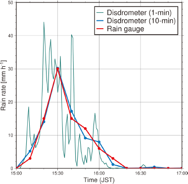
Time series of rainfall rates from the disdrometer (1-min average in green, 10-min average in blue) and the rain gauge at the Kumagaya site (10-min average in red), observed on 11 July 2021.
After the validation of radar rainfall estimates, we examined the correlation between the peak ZDR column height and the maximum rainfall rate near ground level. The resultant correlations between the two are plotted in Fig. 8, in which the horizontal and vertical axes respectively represent the height above the 0 °C level and the maximum rainfall rate observed at the lowest elevation angle of 0.7°.

Scatter plots of peak ZDR column height above the 0 °C level vs. the maximum rainfall rate at low levels, observed on 11 July 2021, with the color scale representing the lag time between observations. Black circles denote the data for Columns A and B, and the red line shows the linear regression. The regression equation and the correlation coefficient are shown in the lower right corner.
According to the regression analysis results, the regression line is represented as
 |
where x is peak column height (km) and y is maximum rainfall rate (mm h−1) near ground level. Although the correlation coefficient is not very high, at 0.64, this result indicates that a taller ZDR column is likely linked to greater production of rainfall. The figure also depicts lag times between observations of peak column height and maximum rainfall rate. About 60 % of the lag times for the thirteen columns were recorded within 8–12 minutes.
In Fig. 8, Column A has a relatively small residual in the linear regression and a normal lag time of 11.5 minutes among them. By contrast, a data point in another sample column, called “Column B” hereinafter, deviates considerably from the regression line, with the longest lag time of 24 minutes. In the following section, we discuss the evolution of both columns, observed within the rectangular areas in Fig. 9, and the cause of the above deviation.

PPI scan of ZDR at 3.8° elevation angle performed by the Haneda radar at 15:02 JST on 11 July 2021. The base map was obtained from the GSI. (a) A snapshot of Column A. Black arcs indicate 50-km and 100-km distances from the radar. Black rectangle (1 × 20 km) and letter “L” respectively denote the analyzed area and the starting point to count the horizontal distance in Figs. 10 and 11. (b) A snapshot of Column B. Black arcs indicate 150-km and 200-km distances from the radar. Black rectangle (1 × 20 km) and letter “L” respectively denote the analyzed area and the starting point to count the horizontal distance in Fig. 13.
Recent studies have shown that a tall ZDR column appears when a sufficiently strong updraft lofts large raindrops well above the 0 °C level during the development of convective clouds, and that as the column decays after reaching a peak height, an area of high rainfall rates aloft descends to the ground (e.g., Kumjian et al. 2014). Figures 10 and 11 both depict the time evolution of Column A, beginning with the observation time of the peak column height and ending with that of the maximum rainfall rate. The 3-dB ZDR contour is superimposed over the field of ZH, ZDR, KDP, and ρHV in Fig. 10, and over that of the highest rainfall rates within a 1-km-wide range of the analyzed area in Fig. 11. The observation time at an elevation angle of 3.8° is shown in the upper left corner of each figure. Note that the cross-sections are reconstructed from several elevation-angle scans, thereby involving some degree of interpolation. In Fig. 10, the areas of high ZH, ZDR, and KDP with low ρHV at heights above the 0 °C level suggest the presence of large raindrops lofted by strong updrafts. In Figs. 11a–c, the areas of maximum rainfall rates gradually descend to the ground as the column decays. Figure 12 shows that the momentary maximum rainfall rate was observed 12 minutes after the column height reached a peak, at 15:14 JST, using the data at the lowest elevation angle of 0.7°. Note that the time is about two minutes later than that shown in Fig. 11c because of the difference in the angles.

Vertical distributions of ZH overlaid with a ZDR contour of 3 dB (solid black), KDP contours of 2 and 4° km−1 (solid green), ρHV contours of 0.9 and 0.95 (solid white), the environmental 0 °C level of 4.6 km AGL (dashed black), and the observation time at 3.8° elevation angle in the upper left corner, representing the evolution of Column A. The horizontal axis represents the distance from the point denoted by the letter “L” in Fig. 9a. Note that Column A is the lower one with a height of 4.6 km AGL in (b).


Time series of the maximum rainfall rates within 5–30 minutes after the peak height of Column A was observed at 15:02 JST at 0.7° elevation angle. The red line indicates the observation time of the momentary maximum rainfall rate.
Figure 13 depicts the time evolution of Column B, which has different characteristics from other columns (Fig. 8) and considerably high rainfall rates above the 0 °C level, especially at 15:22 JST (Fig. 13c). The presence of hail is expected at these levels at sub-zero temperatures, which is not taken into account in the rainfall estimation algorithm (Section 3.2). For this reason, the rainfall rates estimated for Column B are likely to be inaccurate. To confirm this inference, we examined the vertical distributions of KDP, ρHV, and R(KDP, ZH) as in Fig. 14, modified from Fig. 13c. The areas of high KDP overlap only slightly with those of R(KDP, ZH) ≥ 150 mm h−1, denoted by the dashed contour, which reveals that the estimates of high rainfall rates are in error due to R(ZH) being included in the measurement, caused by low KDP and high ZH. In other words, the mismatch of high KDP and high R(KDP, ZH) implies incorrect radar rainfall estimation. Moreover, the areas of low ρHV superimposed with bold contours nearly overlap those of high R(KDP, ZH), which indicates that hail is present in those areas, since ρHV decreases in hail-mixed precipitation (Kumjian 2013a). The presence of hail is, therefore, likely to have caused the estimation error by increasing ZH but leaving KDP unaffected.


Vertical distribution of KDP calculated for Column B, overlaid with a ρHV contour of 0.86 in bold black, R(KDP, ZH) contour of 150 mm h−1 in dashed black, and the observation time in the upper left corner.
To reduce the effect of interference from hail, we recalculated low-level maximum rainfall rates after eliminating data with R(KDP, ZH) > 1.5R (KDP) and R(KDP, ZH) > 100 mm h−1 to detect heavy precipitation estimates that are strongly affected by the presence of hail. The recalculation led to an approximately 50 % change in Column B but less than 15 % for the other columns in the resultant maximum rainfall rates. Note that this algorithm is applicable only to hail-mixed heavy rainfall estimation and does not work for pure rain. The regression equation and the correlation coefficient between rainfall estimates from radar and disdrometer are
 |
where x is the rainfall rate derived from disdrometer (mm h−1) and y is that from radar (mm h−1). They are approximately equal to those shown in Fig. 6b, which supports the validity of the algorithm.
Figure 15 shows the correlations between the peak ZDR column height and the maximum rainfall rate near ground level, where the recalculated results for Columns A and B are denoted as Columns A′ and B′, respectively. The equation of the regression line alters from Eq. (3) to
 |
and the correlation coefficient changes to 0.61 because of the great reduction in the covariance between ZDR column height and low-level maximum rainfall rate.

As in Fig. 8, but the data are recalculated after eliminating those affected by hail. Solid black circles denote the data for Columns A′ and B′. For reference, the dashed black circle denotes the original data for Column B, and the dashed red line shows the linear regression before recalculation.
We explored lag times between observations of the peak column height and the maximum rainfall rate as a function of peak column height, as plotted in Fig. 16, where no correlation is shown, although enhanced ZDR suggests the presence of large raindrops. Instead, most of the lag times were 9–12 minutes regardless of height, and the mean (standard error) was 11.1 (± 1.06) minutes. Assuming that it takes several minutes for raindrops to fall from the level of the lowest elevation measurement with the radar to ground level, the expected forecast lead time is about 13–15 minutes, which precisely matches the peak lag correlation time arrived at by numerical simulation in Kumjian et al. (2014). The figure also suggests that convective clouds with ZDR columns over 3 km tall have the potential to produce extreme rainfall with an intensity of over 180 mm h−1 at ground level.

Scatter plots of peak ZDR column height above 0 °C level vs. lag time between peak column height and maximum rainfall rate observations, with the color scale representing maximum rainfall rates. Black and red lines respectively indicate 3 km height and mean lag time (11.1 min), and solid black circles denote the data for Columns A′ and B′.
To validate the findings from the quantitative analysis on the thirteen columns, we looked at nine ZDR columns observed by the Haneda radar above the estimated 0 °C level of 5.9 km AGL on 12 August 2020, about 1 km higher than that on 11 July 2021. In Fig. 17, the peak column height is positively correlated with the maximum rainfall rate near ground level, and the correlation coefficient is 0.62.
Figure 18 shows the correlation between the two, calculated using both data collected on 11 July 2021 and 12 August 2020. The equation of the regression line is
 |
where x is peak column height (km) and y is maximum rainfall rate (mm h−1) near ground level. The correlation coefficient is 0.68, the highest value in this study. These results suggest that the quantitative relationship obtained in this study is applicable to other rainfall events and that rainfall intensity is likely to exceed 50 mm h−1 when radar identifies a ZDR column over the Kanto region in summer.

As in Fig. 8, but the data were observed on 12 August 2020.

Scatter plots of peak ZDR column height above the 0 °C level vs. the maximum rainfall rate at low levels. Blue circular and green triangular dots respectively represent the data collected on 11 July 2021 and those on 12 August 2020. The red line shows the linear regression, and the regression equation and the correlation coefficient are shown in the upper right corner.
The correlation between the peak column height and the lag time, calculated using the data collected on 12 August 2020, is shown in Fig. 19, in which those on 11 July 2021 are not plotted because of the difference in the estimated 0 °C levels. According to the regression analysis results, the regression line is represented as
 |
where x is peak column height (km) and y is lag time (min). The figure shows a positive correlation with a coefficient of 0.68, which is likely associated with the correlation between ZDR column height and updraft intensity. However, no correlation is shown in Fig. 16. Further analysis of cases in various atmospheric conditions is needed to arrive at a definitive understanding of the difference in correlations between them.

As in Fig. 16, but the data were observed on 12 August 2020. The red line shows the linear regression, and the regression equation and the correlation coefficient are shown in the lower right corner.
The increasing use of dual-polarization radar in recent decades has allowed progressive elucidation of the characteristics of ZDR columns. For example, growth in the volume of a ZDR column appears before an increase in radar reflectivity at low levels (e.g., Picca et al. 2010). The location and height of a ZDR column are closely related to the position and intensity of updrafts, respectively (e.g., Snyder et al. 2015). Although ZDR columns are increasingly regarded as a predictive tool for extreme rainfall, it remains unclear how well they are associated with rainfall intensity on the ground and to what extent they can be applied to weather prediction.
Our quantitative research using dual-polarization radar measurements reveals a positive correlation between peak ZDR column height and maximum rainfall rate near ground level, indicating that ZDR columns should be able to provide useful information on expected rainfall intensity. For instance, when radar identifies a ZDR column, rainfall intensity on the ground is likely to exceed 50 mm h−1 and continue to increase while the column grows in height. A column over 3 km tall from the environmental 0 °C level can be a precursor of extreme rainfall with an intensity of 180 mm h−1 or more. The heaviest rainfall is likely to occur about 10–20 minutes after a ZDR column matures, though more studies are required to determine the definitive forecast lead time. Our findings suggest that ZDR column measurement can help to improve very short-range forecasts and/or nowcasts and lead to early warnings and better disaster management of localized rainfall extremes and the damaging floods that result from them.
On the other hand, the resultant correlation might be improved by applying additional meteorological data or environmental factors. As an example, certain convective parameters, such as convective available potential energy (CAPE), may strengthen the correlation if integrated into the data analysis. Additionally, with further studies on ZDR columns, a better understanding of cloud microphysical processes in convective clouds might, for instance, contribute to the development of numerical weather prediction models through the identification of updraft regions. In brief, more advanced research is needed in future to enhance the effectiveness of operational applications of ZDR columns for severe weather prediction.
The Parsivel disdrometer records rainfall rates derived from its onboard ASDO software, but they tend to be overestimated during heavy rainfall events (Thurai et al. 2011). Adachi et al. (2013) suggest that this tendency is likely to occur because the diameters determined by Parsivel1 are not volume-equivalent: they are only the maximum horizontal diameters of particles. For this reason, we recalculated rainfall rates using DSD data obtained through converting horizontal diameters of raindrops into volume-equivalent versions on the basis of the model axis ratio presented by Beard and Chuang (1987) and reducing the influence of strong wind and turbulence as proposed by Friedrich et al. (2013). The equation for calculating rainfall rates is expressed as
 |
where R is rainfall rate (mm h−1), Cp and Dp are the number and the volume equivalent diameter (mm) of the particles in the 32 size classes, S is the measuring area (m2), and Δt is the sampling time (s).
The observational data from radar and disdrometer measurements analyzed in this study, which respectively belong to the Japan Meteorological Agency (JMA) and Meteorological Research Institute (MRI), are available from the corresponding author upon reasonable request. The precipitation data from the rain gauge is available at https://www.data.jma.go.jp/gmd/risk/obsdl/index.php (in Japanese).
The authors would like to thank Professors Michiko Otsuka, Tomoyuki Kamakura, and Takahiro Ito at Meteorological College for their support and assistance. We are grateful for the constructive comments from Drs. Teruyuki Kato, Hiroshi Yamauchi, Akihito Umehara, and Takashi Unuma of MRI. Drs. Nobuhiro Nagumo, Yusuke Kajiwara, Akira Ooshima, Shuichi Tanaka, and Sohei Yoneda of the JMA’s Atmosphere and Ocean Department and others also helped us to improve the quality of this work. Data from the Haneda and Narita radar stations are courtesy of the JMA and were analyzed using Draft (Tanaka and Suzuki 2000). Lastly, the first author thanks an English checker, Mr. Eric Sheldon, and her mother, Mrs. Miwako Otsubo, for their heartfelt support.
This work was supported in part by JSPS KAKENHI, Grant Number JP20K04092, and by the Workshops and Symposia (2022K-03), a collaborative research of the Disaster Prevention Research Institute, Kyoto University. The manuscript was greatly improved thanks to two anonymous reviewers.