Article
Emergence of Future Sea-Level Pressure Patterns in Recent Summertime East Asia
2024 Volume 102 Issue 2 Pages 265-283

Details
2024 Volume 102 Issue 2 Pages 265-283
Recent year-to-year and long-term climate variabilities during 1980 – 2020 were investigated using the Japanese 55-year reanalysis dataset (JRA-55) to assess the robustness of and uncertainties in future sea-level pressure (SLP) patterns for summertime East Asia due to global warming, which were obtained in a previous study by an inter-model empirical orthogonal function (EOF) analysis of the multi-model future projections in the sixth phase of the Coupled Model Intercomparison Project (CMIP6). One major finding is that the future robust SLP pattern emerges with a significant trend in the recent long-term variability consistent with the CMIP6 future projection. A few of the future uncertain patterns also display significant trends recently, but against the future projection means. The year-to-year variability of the patterns tends to make the polarized extreme summer SLP variations through the superposition with the long-term trends.
The second EOF pattern reflects low- and high-SLP anomalies in northern and southern East Asia, respectively, which is a robust future SLP pattern as its future appearance is predicted by almost all CMIP6 models. While the pattern appears in the summer following an El Niño winter, the significant trend in the recent long-term variability is created similarly to the CMIP6 future projection by recent warming over northern continents and seas.
The other EOFs are the uncertain future SLP patterns as the future polarities depend on the CMIP6 projection model. The first and third patterns represent a strengthened high-pressure anomaly and a weakened southerly wind pattern over East Asia, respectively. They show small linear trends in the magnitude consistent with the small future changes. The high-ranked patterns display long-term decreases against each future ensemble mean. The trends in the uncertain patterns are attributed to the weak and reverse surface warming distribution over the tropical oceans in the recent climate change compared with the future change.
Studies of regional climate change under global warming conditions are becoming increasingly important for mitigation policies. However, such climate change in East Asia is not well understood. For example, the “wet-getting-wetter” effect (Held and Soden 2006) is not enough for explaining future regional precipitation changes. A large part of the uncertainty associated with future precipitation change in East Asia is due to changes in regional atmospheric circulation (Ose 2017, 2019; Zou et al. 2018). Ito et al. (2020) investigated the fifth phase of the Coupled Model Intercomparison Project (CMIP5) ensemble projections (Taylor et al. 2012), and showed that future changes in regional surface air temperature and precipitation over Japan can be diagnosed by surface wind changes analyzed from future sea-level pressure (SLP). Endo et al. (2018) used CMIP5 simulations to show that the effects of land and ocean on the future Asian summer monsoon are quite different: warming land strengthens southerly winds over the East Asian continent and neighboring seas, whereas a warmer sea surface temperature (SST) weakens East Asian monsoonal circulation by suppressing vertical motion over the Indian and Pacific oceans. Endo et al. (2021) also examined future changes in the seasonal nature of the East Asian monsoon by performing various experiments with the Meteorological Research Institute – Atmospheric General Circulation Model (MRI-AGCM) (Mizuta et al. 2012), and showed that the warming of the northern continental summer (including neighboring seas) is also significant for projecting East Asian future climate in addition to tropical and global SST warming, especially for late summer.
The western North Pacific subtropical high (WNPSH) is a key element of the East Asian summer monsoon. Its recent trends and long-term changes were analyzed by Matsumura et al. (2015) and Matsumura and Horinouchi (2016). The SST trends, and El Niño-Southern Oscillation (ENSO) and decadal SST variabilities are suggested as the environments causing specific mechanisms such as changes in summer rainband activity. Various storyline approaches (Shepherd 2019) are studied for changes in the East Asian subtropical high in summer. Choi and Kim (2019) analyzed the major modes of summertime variability of the WNPSH by applying the cyclo-stationary empirical orthogonal function (EOF) method to the monthly 500 hPa geopotential stationary height during 1979 – 2017, and found that the leading mode is a clear strengthening of the WNPSH associated with global warming. Zhou et al. (2020) applied the EOF method to normalized multi-fields consisting of upper- and lower-level circulations in the CMIP5 and the sixth phase of the Coupled Model Intercomparison Project (CMIP6) projections (Eyring et al. 2016), in order to assess the inter-model spread of future changes in the East Asian summer monsoon system. Chen et al. (2020) investigated the leading modes of uncertainty in the future summer WNPSH by applying the EOF method to CMIP5 representative concentration pathway (RCP) 8.5 multi-model ensemble experiments, and attempted to determine the emergent constraints on the WNPSH, based on model biases. The variability of the WNPSH under global warming conditions was studied by Yang et al. (2022), who concluded that the frequency of strong WNPSH events will increase in the future due to the stronger response of tropical atmospheric convection to the central Pacific low-SST anomaly.
Ose et al. (2020, 2022) applied EOF analysis to future changes in summertime East Asian SLP changes in the 38 CMIP5 projections for the RCP 8.5 scenario and the 38 CMIP6 projections for the shared socioeconomic pathways (SSP) 5–8.5 scenario, respectively. These studies not only focused on the leading EOF mode, but also on the first six EOF modes, given that the source of the modes reflects different aspects unique to global warming, such as the distributions of SST and continental warming, and regionally suppressed vertical motion. As a result, the second EOF pattern characterized as low- and high-SLP anomalies in northern and southern East Asia respectively was recognized to be the robust SLP pattern, meaning that almost all CMIP6 and most CMIP5 models project the appearance of that SLP pattern in future East Asian climate change. The future appearance of this pattern was attributed to the warming of northern continents and neighboring seas. The future polarity of the other EOF patterns is dependent on the model, indicating that these are uncertain future SLP patterns.
These aforementioned results were obtained from the future global warming projection with the CMIP6 models. A question is left: how reliable the future SLP EOF pattern’s appearance and their physical mechanism are in the real. A part of the answer could be obtained by studying how year-to-year variations, long-term variability, and climate changes of the future SLP patterns are appearing in recent observation-based analyses and what kinds of the environments are accompanied with the recent variations of the future SLP patterns. The objectives of this study were to address these questions, and examine if the SLP EOF patterns from the future CMIP6 projections (Ose et al. 2022) are evident in recent climate data. The results of this study may reduce the uncertainty of future SLP projections and associated fields in the East Asian summer.
An example for the reduced uncertainty based on the study on recent climate change is found in Tokarska et al. (2020), who tried to choose the reliable future projections for the global mean surface temperature change in the CMIP6 experiments by comparing the observed and simulated past temperature changes from 1981 to 2017 and then constraining the reliable future changes for the 2081 – 2100 mean. In this study, the similar future constraints are tried to study by comparing the observed and simulated past variability of the future SLP patterns in East Asia from 1980 to 2014.
The observation-based analysis on the actual year-to-year variability is also useful for measuring the impacts of the recent long-term variability and the future change in the SLP patterns. If the recent long-term variability and the future change are small in magnitude compared with the actual year-to-year variability, the impact of the climate change will be small. If not, the superposition of the long-term climate changes and the year-to-year variability may create inexperienced extreme summers. In this case, it becomes important to know not only how the long-term variability and the future change occur but also how the year-to-year variability happens in the real.
The remainder of this manuscript is organized as follows. The data used in our analysis are introduced in Section 2, and the results are described in Section 3. A discussion is presented in Section 4, followed by conclusions in Section 5.
The future SLP patterns used in this study were obtained from the inter-model EOF analysis of Ose et al. (2022), in which 38 CMIP6 models’ historical and SSP5-8.5 scenario experiments were used. The difference between the two sets of 20-year simulations for the “present day” (1980 – 1999) and “future” (2076 – 2095) periods is defined as “future change.” The future changes by each model were adjusted to values accounting for an annual mean global warming of 4 K, using the future projection of the 20-year annual global mean surface air temperature. The inter-model EOF analysis was applied to the future SLP changes in the East Asian EOF domain [10 – 50°N, 110 – 160°E] for the 38 CMIP6 models, which is the region used for the definition of the southerly wind index in East Asia in Fig. 14.5 of IPCC (2013). The detailed method of the inter-model EOF analysis in Ose et al. (2022) is summarized in Appendix A.
The first to sixth inter-model EOF modes (EOF1 – 6) of the CMIP6 multi-model future SLP changes in summertime East Asia (dslpEOF1-6 in Ose et al. 2022 or Appendix A) are shown for reference with contours over the East Asian EOF domain in Figs. 1a – f, after multiplying by the first to sixth inter-model standard deviation (SD1 – 6 in Appendix A), which have values of 10.354, 4.554, 3.664, 2.559, 2.087, and 1.901 hPa, respectively. The ratios of the inter-model variance explained by EOF1 – 6 to the total variance within the EOF domain are 65.6, 12.7, 8.2, 4.0, 2.7, and 2.2 %, respectively.

(a; color) Recent year-to-year correlations during 1980 – 2020 between the JJA-mean sea-level pressure and the EOF1 resolution coefficient (empty bars in Fig. 2a) using the JRA-55 reanalysis dataset, and (contour interval = 0.2 hPa) the EOF1 pattern multiplied by its CMIP6 inter-model standard deviations. A square enclosed with a thick line represents the EOF domain. (b) – (f) Same as (a), except for EOF2 – 6. Correlation coefficients of 0.3 and 0.4 indicate statistical significance at the > 95 % and > 99 % levels, respectively.
We analyzed year-to-year and long-term climate variations and climate change in summer (June–July–August mean; JJA mean) in East Asia during the “recent” period (1980 – 2020) using the Japanese 55-year reanalysis (JRA-55; Kobayashi et al. 2015) and Global Precipitation Climatology Project (GPCP ver. 2.3; Adler et al. 2003) datasets. The recent climate variations and the recent climate change are analyzed for the deviation from the “present-day” (1980 – 1999) mean. All data used in this study were re-gridded to a resolution of 2.5° longitude × 2.5° latitude.
We also used the seasonal mean index data for the recent SST variability (Japan Meteorological Agency 2023) such as NINO1+2, NINO3, NINO4, and IOBW for SST over the domains of [EQ. − 10°S, 90 − 80°W], [5°N − 5°S, 150 − 90°W], [5°N − 5°S, 160°E − 150°W], and [20°N − 20°S, 40 − 100°E], respectively. These are referred to by abbreviations, such as ‘NINO3 SST Index.’
Recent year-to-year variations in the future SLP patterns are defined as the recent year-to-year variations in the resolution coefficients of the summer JRA-55 SLP anomaly resolved by the future normalized EOF1 – 6 patterns derived from the CMIP6 data. The calculation of the resolution coefficients of the JRA-55 SLP anomaly is introduced in Appendix B. Simply mentioned, the resolution coefficient for a summer represents how much the SLP pattern in the summer includes the future SLP pattern regarding both the similarity and magnitude of pattern. The year-to-year EOF resolution coefficients of the JRA-55 SLP deviation from the “present-day” (1980 – 1999) mean are plotted for the recent period (1980 – 2020) in Figs. 2a – f, along with the 7-year running means. The standard deviations for the recent year-to-year variations in the EOF1 – 6 resolution coefficients are 0.92, 1.24, 1.15, 1.82, 1.80, and 1.45, respectively, in the normalized unit. These are relatively large for the high-ranking EOF modes, as compared with the inter-model uncertainty of the future EOF changes (1.0 in the graph units), which is probably due to their small spatial structures.
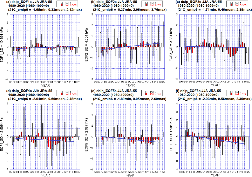
(a) Recent year-to-year variations in resolution coefficients during 1980 – 2020 for (empty bars) the EOF1 pattern of future sea-level pressure changes in East Asia and (red-filled bars) their 7-year running means. A blue line is the linear trend for the 7-year means. (b) – (f) Same as (a), but for EOF2 – 6. Units on the vertical axis are divided by the CMIP6 inter-model standard deviation of each EOF, which is noted along the vertical axis. The same unit is used for the CMIP6 future ensemble minimum, mean, and maximum changes of the corresponding EOF resolution coefficient, which are noted in the title of each graph.
The 7-year running mean (7-year-mean) represents the long-term variability of each EOF resolution coefficient of the JRA-55 SLP deviation after averaging typical ENSO variability with the period of 2 – 6 years. The 7-year-mean of EOF2 resolution coefficients forms a significant linear trend as confirmed by the statistics later. This trend of about +1.85 (100 yr)−1 is broadly quantitatively consistent with the CMIP6 ensemble mean EOF2 future change of 2.06 in terms of the normalized unit.
The future ensemble-mean changes in the EOF1 and EOF3 – 6 resolution coefficients of the CMIP6 SLP projection were 0.325, 0.457, 0.656, 0.046, and 0.555, respectively, in terms of the normalized units, which are small as a result of the uncertain future EOF modes (Ose et al. 2022). The EOF1 resolution coefficients of the JRA-55 SLP deviation exhibit no significant trend during the recent period (1980 – 2020). Long-term variability characterizes the EOF3 time-series of the JRA-55 SLP, with a similar amplitude to the future ensemble mean change of the CMIP6 SLP.
The statistics for the linear trends in the 7-year-means of the EOF1 – 6 resolution coefficients during 1980 – 2020 are summarized in Table 1, where the least square method is applied for calculating the linear trends. The student’s t-test for the null-hypnosis supports the linear trend in the 7-year-mean variability of the EOF2 resolution coefficients with more than 98 % significance, compared with less than 80 % significance for EOF1 and EOF3, assuming the degree of freedom (n – 2 = 5 – 2) because the recent period of the 41 years includes five independent 7-year-means at least. The small determination rates less than 10 % for EOF1 and EOF3 suggest relatively large fluctuations with time around the calculated linear trends.

The EOF4 – 6 resolution coefficients of the JRA-55 SLP typically exhibit negative deviations as compared with the positive future mean changes in the corresponding CMIP6 SLP EOF patterns, suggesting that the future mean projections may be incorrect or that there is large internal variability on these EOF4 – 6 patterns. The statistics in Table 1 indicate that both the EOF5 and EOF6 resolution coefficients of the JRA-55 SLP variability show significant but negative trends against each future ensemble mean.
The anomaly correlation between the year-to-year EOF resolution coefficients of the JRA-55 SLP (Figs. 2a – f) and the JRA-55 SLP anomaly field during the recent period (1980 – 2020) is shown in Figs. 1a – f. The method for the calculation of the anomaly correlation between the year-to-year EOF resolution coefficients (Figs. 2a – f) and any recent fields such as the JRA-55 SLP field and the GPCP data is given in Appendix B. The correlation patterns with the JRA-55 SLP field are broadly similar to the corresponding SLP EOF patterns, except that the high positive correlations for the EOF1 – 2 resolution coefficients of the JRA-55 SLP anomalies are slightly shifted from the EOF patterns to north of the Philippine Islands. The resolution coefficients of the SLP EOF1 and EOF2 are mathematically calculated mostly by depending on whether large scale patterns of the JJA SLP anomalies tend to keep a single polarity entirely over the EOF domain or they tend to have different polarities in the northern and southern areas of the EOF domain. However, the year-to-year correlation analysis using the JRA55 recent data shows that the JJA SLP anomalies displaying the large resolution coefficients of the SLP EOF1 and EOF2 tend to have the similar small spatial structures to north of the Philippine Islands on the corresponding EOF patterns. The reason is explained in the next subsection.
3.2 Recent year-to-year variations in other fieldsFuture changes in surface air temperature and vertical motion were proposed by Ose et al. (2022) as the sources to explain the appearance of the CMIP6 SLP EOF1 – 3 modes in the future global warming. Figures 3a – c show the year-to-year correlations of the EOF1 – 3 resolution coefficients of the JRA-55 SLP anomalies with the JRA-55 surface air temperature anomalies, along with the corresponding CMIP6 inter-model analysis for the future changes (Ose et al. 2022). There are no clear similarities between the JRA-55 year-to-year variations and the CMIP6 future changes, apart from a few features: (1) a negative SST correlation along the equatorial central Pacific and a positive SST correlation in the tropical northern Atlantic for EOF1; and (2) a positive SST correlation in the subtropical northern Pacific for EOF3 (in both cases assuming that the SST anomalies are close to the surface air temperature anomalies). The year-to-year correlations of the JRA-55 SLP EOF resolution coefficients with the previous northern winter (December–January–February mean; DJF mean) surface air temperature are shown in Figs. 3d – f. The recent year-to-year variations in EOF1 – 2 exhibit the summer Asian monsoon anomalies after an El Niño winter (e.g., Ose et al. 1997; Xie et al. 2009), which are specifically warmer SST anomalies in the northern Indian and tropical northern Atlantic oceans (Figs. 3a, b), as well as the high-pressure anomalies to north of the Philippine Islands (Figs. 1a, b). Note that the recent JJA year-to-year variations in EOF1 and EOF2 are significantly related to the previous DJF NINO4 SST Index with the correlation of 0.42 and the DJF NINO3 SST Index with 0.43, respectively. The similar future changes between the JJA and DJF SST anomalies for the CMIP6 EOF1 – 3 correlations indicate that the future SST changes are annually unchanged. A warm SST anomaly in the subtropical northwestern Pacific for EOF3 is caused by the EOF3 surface circulation anomaly in the JRA55 year-to-year correlations as suggested for the CMIP6 future changes (Ose et al. 2022). Warm SST anomalies in the eastern Pacific of the JRA-55 analysis for EOF3 may be related to the recent variability of the year-to-year EOF3 resolution coefficient (Fig. 2c).

(a) – (c) (Colors) Recent year-to-year correlations during 1980 – 2020 between the JJA-mean surface air temperature and the EOF1 – 3 resolution coefficients (empty bars in Figs. 2a – c) using the JRA-55 reanalysis dataset, and (contours of −0.6, −0.4, −0.3, 0.3, 0.4, and 0.6) the same for the 38 CMIP6 inter-model correlations of the CMIP6 future changes. (d) – (f) Same as (a) – (c), except for (colors) the previous DJF surface air temperature and (contours) the CMIP6 future changes in the mean DJF one. Correlation coefficients of 0.3 and 0.4 indicate statistical significance at the > 95 % and > 99 % levels, respectively.
Figures 4a – c show the year-to-year correlation of the EOF1 – 3 resolution coefficients with the JRA-55 vertical velocity that is the pressure – time derivative at 500 hPa (positive/negative values indicate downward/upward motions). The corresponding analysis of the future changes is indicated by contours in Figs. 4a – c. The year-to-year correlations for EOF1 – 2 have similar features to the post- El Niño summer Asian monsoon, such as downward motion anomalies north of the Philippine Islands. Differences between EOF1 and EOF2 can be found in a significantly organized upward motion anomaly around the maritime continent and a downward motion anomaly over the equatorial Pacific for EOF1, but not EOF2. These features are also evident for the corresponding analysis of the future changes.

(a) – (c) (Colors) Recent year-to-year correlations during 1980 – 2020 between the JJA-mean vertical downward velocity (pressure velocity) and the EOF1 – 3 resolution coefficients (empty bars in Figs. 2a – c) using the JRA-55 reanalysis dataset (colors) and the same for the 38 CMIP6 inter-model correlations for the CMIP6 future changes (contours of −0.6, −0.4, −0.3, 0.3, 0.4, and 0.6). (d) – (f) Same as (a) – (c), except for the GPCP JJA-mean precipitation and (contours) CMIP6 future changes in JJA-mean precipitation. Correlation coefficients of 0.3 and 0.4 indicate statistical significance at the > 95 % and > 99 % levels, respectively.
The GPCP precipitation was used for the year-to-year correlation analysis (Figs. 4d – f) to support the analysis of vertical velocity (Figs. 4a – c), which is not generally thought to be as reliable as the temperature and horizontal winds. The year-to-year correlations of GPCP precipitation and JRA-55 vertical velocity for EOF2 have a similar geographical distribution (colors in Figs. 4b, e). However, as detected over the subtropical northwestern Pacific in the CMIP6 future inter-model analysis of EOF2 (contours in Figs. 4b, e), the future changes in precipitation are not necessarily the same as the geographical pattern of vertical velocity, given the additional contribution from future moisture change to precipitation.
Significant year-to-year correlations between GPCP precipitation and EOF1 (Fig. 4d) were confirmed over the maritime continent, the equatorial western Pacific, and the tropical northwestern Pacific. Similar correlations between EOF1 and future precipitation changes are also evident (Fig. 4d). The significant high correlations over northwestern South Asia can be detected for EOF1 in both the GPCP year-to-year variations and the CMIP6 future inter-model analysis of precipitation (Fig. 4d), but not for the vertical velocity (Fig. 4a). The moisture transport into northwestern South Asia may be strengthened by the EOF1-related lower circulation anomaly for the JRA-55 year-to-year analysis and the CMIP6 future analysis (Figs. 1a, 2a of Ose et al. 2022).
The common features between the year-to-year variations and the future changes are confirmed outside the East Asia EOF domain for the EOF1 correlations with the upward motion, precipitation, and the equatorial Pacific SST, indicating that common physical mechanisms are involved. Naoi et al. (2020) investigated the differences in the meridional position of the atmospheric river over East Asia in the summer during the rapid seasonal transition after an El Niño winter. Based on Fig. 7 of Naoi et al. (2020), the northward expansion of the SLP EOF1 anomaly over East Asia may be explained by the atmospheric response to diabatic heating (or upward motion) over the maritime continent and eastern Indian Ocean (Figs. 4a, d), but this is not clear in the SLP EOF2 anomaly (Figs. 4b, e).

(a; colors) The 20-year mean change in JJA-mean sea-level pressure (hPa) from 1980 – 1999 to 2001 – 2020 (colors), and (contours) the 20-year mean climatology during 1980 – 1999 relative to 1000 hPa. (b) Same as (a), except for the 20-year mean change in the JJA- and DJF-mean surface air temperature (colors and contours of −0.5, 0.0, and 0.5 K, respectively). (c) Same as (a), except for the JJA-mean vertical downward velocity (pressure velocity) (hPa h−1). (d) The JJA-mean 200 hPa zonal wind (m s−1). (e) The JJA-mean vertical dry static stability is defined as the difference between the dry potential temperature at 200 hPa and 700 hPa (K). An elevated area of less than 700 hPa is enclosed by green lines. (f) The JJA-mean GPCP precipitation (mm day−1). (a) – (e) are based on the JRA-55 reanalysis dataset.

(a; colors) The 20-year mean future change in JJA-mean sea-level pressure (hPa) from 1980 – 1999 to 2076 – 2095 and (contours) the 20-year mean climatology during 1980 – 1999 relative to 1000 hPa, based on the 38 CMIP6 ensemble mean simulations. (b) Same as (a) except for the JJA-mean surface air temperature in K with contours every 0.2 K between 3.0 K and 4.0 K. (c) The JJA-mean vertical downward velocity (pressure velocity) (hPa h−1). (d) The JJA-mean 200 hPa zonal wind (m s−1). (e) The JJA-mean vertical dry static stability, is defined as the difference between dry potential temperature at 200 hPa and 700 hPa (K). An elevated area less than 700 hPa is enclosed by green lines. (f) The JJA-mean precipitation (mm day−1).

(a) Recent changes in the EOF1 resolution coefficients in the 38 CMIP6 historical experiments from 1980 – 1999 to 2000 – 2014 (horizontal axis) and their future changes from 1980 – 1999 to 2076 – 2095, based on the 38 CMIP6 SSP5-8.5 experiments (vertical axis). (b) – (f) Same as (a), but for EOF2 – 6. Red lines are the CMIP6 inter-model linear regressions between recent and future changes. Red-filled circles are the CMIP6 ensemble means. Red empty squares are the JRA-55-based recent changes from 1980 – 1999 to 2000 – 2014 (horizontal axis) and the regression for 2076 – 2095 (vertical axis).
For EOF3, a similar year-to-year correlation was confirmed for both the GPCP precipitation and JRA-55 vertical velocity near the Philippine Islands (Figs. 4c, f). However, these correlations were not confirmed in the inter-model analysis of the CMIP6 future changes (Figs. 4c, f). The recent variability such as tropical cyclones may be involved in the differences.
The CMIP6 analysis for the EOF4 – 6 SLP patterns, which is totally omitted in Ose et al. (2022), is presented in Supplement. The future SLP EOF4 – 6 patterns come from the inter-model differences in the CMIP6 present-day simulation of the regional vertical velocity (mostly due to regional precipitation) over the sub-tropical and tropical oceans (Figs. S1a – c), which leads to the inter-model differences in the future suppressed vertical motions. Regional GPCP precipitation anomalies detected in the year-to-year correlations of EOF5 and EOF6 are distributed over nearly the same areas in the northwestern Pacific as the future regional upward anomalies of CMIP6 EOF5 and EOF6, respectively (Figs. S1d – f). However, for surface air temperature anomalies of EOF5 and EOF6, weak similarities between the JRA-55 year-to-year variability and the CMIP6 future inter-model anomalies can be found only over the limited areas of the tropical eastern Pacific and the tropical Indian Ocean, respectively (Figs. S2a – c, S2d – f).
The EOF4 SLP pattern is regarded as the atmospheric response to the equatorial Pacific SST anomaly (Fig. S2a) as indicated by the correlation of −0.43 with the JJA NINO4 SST Index. At least, from view of the geographical SLP anomaly patterns, the EOF5 and EOF6 SLP patterns may be similar to the Pacific-Japan (P-J) pattern (e.g., Kosaka and Nakamura 2006 and 2011) and the “convective jump” pattern in the summer northwestern Pacific (Ueda and Yasunari 1996), respectively. It is also a note that EOF4 and EOF5 have significant year-to-year correlations with the previous winter El Niño SST (Fig. S2e) when focused only on the recent period, specifically with the correlations of 0.37 and 0.32 with the DJF NINO1+2 SST Index, respectively.
Reasons for the negative trends in the recent EOF4 – 6 variability are not necessarily clear from the above analysis. A possibility that the recent long-term variabilities of EOF4 – 6 are influenced by the recent climate change in the tropics, which is rather different from that of the CMIP6 future projection, will be shown in Section 3.4.
Another possibility is that the actual EOF4 – 6 displaying small-scale SLP structures in JRA-55 may represent the year-to-year anomaly of the tropical cyclones’ activity in the northwestern Pacific, which are not simulated mostly by the CMIP6 models.
3.3 Summary of the recent variability and future uncertainty in the future SLP patternsIn summary, the common distributions are found in the correlation maps with the vertical velocity mostly between the JRA-55 year-to-year variability and the CMIP6 future inter-model variability. Therefore, the vertical velocity anomalies are recognized as the direct source for the appearance of the SLP EOF patterns. The above fact is not necessarily confirmed for the surface air temperature.
The high-in-the-south SLP anomaly of EOF2 is attributed to the downward motion anomaly as a physical cause for the appearance common between the recent JRA-55 year-to-year variations and the CMIP6 inter-model variations of the future changes. The former is caused by suppressed subtropical northwestern precipitation in the East Asian summer following the El Niño winter, whereas the latter is caused by the suppression of the vertical velocity in the future global warming environment. The low-in-the-north SLP anomaly of EOF2 is caused by the strong warming over the northern continents and neighboring seas in the CMIP6 future projections (Ose et al. 2022), whereas this is not confirmed in the year-to-year variability. However, the 7-year-means of the recent year-to-year variations in the JRA55 SLP EOF2 resolution coefficients have the significant positive trend consistent with the CMIP6 future ensemble mean EOF2 changes.
The high SLP anomaly of EOF1 in East Asia is probably due to both the upward motion anomaly from the maritime continent to the tropical Indian Ocean and the low SST anomaly over the equatorial central Pacific, which are found in common for the recent JRA55 year-to-year variations and the CMIP6 future inter-model uncertainty. The recent year-to-year variation in EOF1 has some fluctuations around the trend so that the trend is not statistically significant but consistent with the small ensemble mean future EOF1 change.
In terms of the low-in-the-east and high-in-the-west SLP anomaly of EOF3, the recent year-to-year variations and the future inter-model uncertainty have different features, apart from the subtropical northwestern Pacific SST anomaly probably influenced by the EOF3 pattern. The recent year-to-year variation in EOF3 is related to the eastern Pacific SST anomaly in the subtropics and tropics and exhibits long-term variations. Its amplitude is comparable with that of the small ensemble mean of the future EOF3 changes.
Significant correlations of the EOF4 – 6 SLP patterns with the JRA-55 year-to-year precipitation anomalies are confirmed in the nearly same areas inside of the EOF domain as those with the CMIP6 future upward vertical velocity changes. The vertical velocity anomalies are recognized as the direct sources for the EOF4 – 6 SLP patterns whereas common features are limited for the regional surface temperature anomalies between the JRA-55 year-to-year variability and the CMIP6 future inter-model uncertainty. The EOF4 – 6 resolution coefficients of the JRA-55 SLP anomalies show the negative departures from the present-day mean. In particular, the EOF5 and EOF6 resolution coefficients display the significant but negative trends, which are not consistent with their CMIP6 future ensemble projection means.
3.4 Recent climate changeThe recent trend of the EOF2 year-to-year variations can be explained by recent global warming. From the climatological differences between the 2001 – 2020 and 1980 – 1999 averages based on the JRA-55 data (Fig. 5), which are referred to as “recent climate change,” the low SLP anomaly in northern East Asia (Fig. 5a) and surface air warming in the northern continents and neighboring seas (Fig. 5b) are clearly evident. These can be regarded as the northern low part of the CMIP6 future EOF2 SLP pattern and the physical source for that low SLP, as pointed out by Ose et al. (2022). A comparison between the recent climate changes based on JRA-55 (Fig. 5) and the CMIP6 future ensemble mean changes (Fig. 6) shows a common geographic feature of enhanced warming over the northern continents and neighboring seas.
The high SLP anomaly corresponding to the southern part of EOF2 is unclear in the recent climate change (Fig. 5a). The associated future cause of the southern part of EOF2, which is the downward motion anomaly in the subtropical northwestern Pacific and increased vertical stability in the tropics (Ose et al. 2022), is also unclear or small in the JRA55 recent climate change data (Figs. 5c, e), as compared with the CMIP6 future climate change (Figs. 6c, e). The enhanced warming in northern East Asia that is evident in the recent climate change data is ∼ 0.5 K and 10 % of the future change of 5 K, whereas the enhanced vertical stability in the tropics in the recent climate change data corresponds to ∼ 0.1 K and is < 1 % of the future increase of 6 K. The recent SST increase is quite small and may even be negative in the tropics (Fig. 5b). The unclear recent climate change in the southern part of the EOF2 SLP pattern may be consistent with the negative SST change over the previous DJF El Niño area (Fig. 3e), as indicated by the recent year-to-year variability.
The recent climate change in the JRA-55 vertical motion (Fig. 5c) is rather different from or nearly opposite to the CMIP6 future change in upward motion (Fig. 6c) while increased precipitation is relatively similar between the GPCP recent climate change (Fig. 5f) and the CMIP6 future change (Fig. 6f). The CMIP6 future change in upward motion (Fig. 6c) has a different distribution from that of precipitation (Fig. 6f). In particular, over a large area of Southeast Asia and the tropical Indian Ocean, these future changes have opposite signs because of the effect of the future increased vertical stability in the tropics (Fig. 6e), which leads to increased precipitation but suppressed upward motion. Compared with the future climate change, the recent climate change in the JRA-55 vertical motion (Fig. 5c) tends to be positively correlated with the GPCP precipitation (Fig. 5f) geographically, which is consistent with the small recent increase in SST (Fig. 5b) and the small vertical stabilization (Fig. 5e) in the tropics.
The JRA55 recent changes in the 200 hPa zonal wind over the tropics (Fig. 5d) are nearly opposite to the CMIP6 future changes (Fig. 6d), consistent with the changes in the vertical motions in the tropics, whereas some similarities could be found between the recent and future changes in the northern extra-tropics. This is consistent with the other results of this subsection, which show the regional effect of global warming is small in the tropics as compared with the northern extra-tropics.
It is noted that the recent climate change includes some EOF1-related aspects such as the upward motion anomaly from the maritime continent to the tropical Indian Ocean and the downward motion anomaly over the equatorial central Pacific (Fig. 5c) as well as the small but positive linear trend of EOF1 (Fig. 2a).
Small-scale structures of the EOF4 – 6 SLP patterns displaying the recent negative trends seem to be included in the recent climate change such as a low SLP change over the Okhotsk Sea, a high SLP change to southeast of the Japanese Archipelago and a low SLP change around the Philippine Islands (Fig. 5a). The recent climate change in the tropical SST may display consistent phases with the negative departures of EOF4 – 6 in the recent climate change; warm JJA SST anomaly in the equatorial central Pacific for negative EOF4 (Fig. S2a), the previous DJF negative SST anomaly in the eastern Pacific for negative EOF5 (Fig. S2e) and negative JJA SST anomaly in the “convective jump area” in the subtropical Pacific (Ueda and Yasunari 1996).
Focused on the significant negative trends of EOF5 and/or EOF6, there is an interesting possibility that they contribute to the modification of “the CMIP6-simulated EOF2” to “the actual EOF2 in JRA-55,” which are the real SLP pattern forced by the warming in the northern continents and seas.
EOF1 and EOF2 for the recent year-to-year variability have some physical similarities with “the observed first and second principal patterns of the detrended JJA 850 hPa stream function’s variability” in the WNPSH [10 – 40°N, 110 – 180°E] obtained by Yang et al. (2022), referred to as PC1_Yang2022 and PC2_Yang2022 in this study, respectively. The positively correlated SST anomalies in the Philippine Sea and the northern tropical Atlantic, and negatively correlated SST anomalies over the equatorial central Pacific are common features of EOF1 and PC1_Yang2022. The positively correlated SST anomalies in the tropical Indian Ocean and South China Sea in the summer following an El Niño winter are common features of the EOF2 and PC2_Yang2022. However, there are some differences. The EOF2 pattern is different from that of PC2_Yang2022 in northern East Asia, probably because of the difference in the EOF domain used for the analysis. The variability centered around northern East Asia tends to be captured by the EOF analysis of this study, because the EOF domain covers the high-latitude regions of East Asia, but with a limited eastward extent. In contrast, the domain of PC_Yang2022 is basically within the northwestern subtropics, but extends to the dateline. A more critical difference is the data used for the analysis. PC1-2_Yang2022 was obtained from an analysis of the de-trended recent year-to-year variability. The EOF1 – 6 in this study were obtained from the CMIP6 future changes, where the regional responses and variations uniquely related to global warming are intensified, such as global-scale land warming and suppressed atmospheric vertical motions.
Choi and Kim (2019) undertook an analysis of summertime variability in the WNPSH [9 – 32°N, 105 – 150°E] and showed that the leading mode of the monthly cyclo-stationary empirical orthogonal function (CSEOF1) is forced by global warming. Ignoring the difference between the 500-hPa geopotential height and SLP patterns, the leading CSEOF1 mode is similar in part to EOF2, but the domain defined for the CSEOF modes is not large enough to capture the distinction between EOF1 and EOF2, and thus CSEOF1 may include the regional variability as represented by both EOF1 and EOF2.
4.2 Emergent constraint based on the future SLP patternsFigure 7 shows the relationships between the CMIP6 recent and future climate changes of EOF resolution coefficients for each CMIP6 model experiment, where “the recent climate change” is defined in this subsection as the difference between the periods of 1980 – 1999 and 2000 – 2014 in the same CMIP6 historical run. Each “CMIP6 recent climate change” was simulated using the specified historical forcings of the CMIP6 project, but other natural fluctuations were also included depending on each model experiment. However, it is confirmed that the correlation between the CMIP6 recent and future climate changes of EOF1 – 6 resolution coefficients is 0.42, 0.61, 0.61, 0.40, 0.49 and 0.63, respectively, which are statistically significant over 98 %.
The JRA-55-based actual “recent climate change” for 2000 – 2014 is treated as one sample of the simulations. The actual “recent climate change” for EOF1 – 3 resolution coefficients is lower than the corresponding ensemble mean of the CMIP6 “recent climate change” for 2000 – 2014, but the differences are small compared with the CMIP6 uncertainty as represented by the 38 simulations. Figure 7 also shows the plausible future climate changes corresponding to the actual “recent climate changes” from JRA-55, which are obtained using the statistical linear regression equations displayed in Fig.7. The plausible future changes of the EOF1 – 3 resolution coefficients are proposed to be 0.20, 1.83, and 0.27, rather than the CMIP6 mean future changes of 0.33, 2.06, and 0.46, respectively, based on the inter-model statistical relationships between the CMIP6 “recent and future climate changes.” The modification due to the constraint for EOF1 – 3 is small and reasonable considering the assumption of the 4K future projection and the comparison with the large CMIP6 simulated diversity.
The JRA-55-based actual “recent climate changes” for EOF4 – 6 are within uncertainties of the CMIP6 “recent climate changes” but much lower than the positive CMIP6 ensemble means, leading to the negative EOF4 – 6 resolution coefficients for the future climate changes based on the linear regressions.
4.3 Recent negative trends in the higher-ranked patternsThe influence of the recent SST changes (Fig. 5b) on the recent long-term variability in the SLP patterns is discussed. There is some evidence that the recent negative trends in the higher-ranked EOFs are created through the same physical mechanism as the corresponding year-to-year variability. For the EOF4 and EOF5 resolution coefficients, the correlations in the 7-year running mean variability (the year-to-year variability) with the previous DJF NINO1+2 SST Index are 0.44 (0.37) and 0.4 (0.32), respectively. Therefore, the decrease in the DJF Niño1+2 SST (Fig. 5b) in the recent SST change is considered responsible for the recent decreases in EOF4 and EOF5 through the same mechanism as the year-to-year variability. The EOF6 has a correlation of −0.36 (−0.30) with the JJA IOBW SST Index for the 7-year running mean variability (the year-to-year variability). The recent long-term decrease of EOF6 may be attributed to the increase in the JJA IOBW SST or the tropical Indian Ocean SST, contrasting with the partially decreasing tropical northern Pacific SST in the recent climate change. This statistical fact is consistent with the tendency of the warm JJA IOBW SST to create a high-pressure SLP anomaly over the subtropical northwestern Pacific (Xie et al. 2009).
In summary, the recent long-term variability of the high-ranked SLP patterns is attributed to the features of the recent SST change in the real, when assuming the same mechanism as the year-to-year relationships between EOF4 – 6 and SST.
4.4 Extreme summer SLP variationsSimply considered, polarized extreme summer SLP variation would come one after another with time as a result of the superposition of the recent trends with the associated year-to-year variability. The first, second, and third maximum of the EOF2 resolution coefficients during the summers of 1980 – 2020 are recorded in 2013, 2020, and 2017 (Fig. 2b) with the positive to marginal DJF Niño4 SST anomalies (0.07, 1.32, and −0.095 in the standard deviation unit). The third minimum of the EOF2 resolution coefficients happen in 2012 with the negative DJF Niño4 SST anomaly (−1.26). The first, second, and third minimum of the EOF5 resolution coefficients occur in 2004, 2010, and 2018 with the negative to marginal DJF Niño1+2 SST anomalies (0.10, −0.01, and −0.87). The second maximum of the EOF5 resolution coefficients is found in 2012 with the negative DJF Niño4 SST anomaly (−0.44). The first, second, and third minimum and maximum of the EOF6 resolution coefficients are not recorded after 2001.
The long-term trends of the high-ranked SLP patterns tend to make the polarized extreme summers through the superposition with the year-to-year variability. The tendency may be relatively stable for the EOF2 because the warming northern continents as the source for the EOF2 trend proceeds independently from the year-to-year variability due to the tropical SST variations.
The recent year-to-year and long-term climate variability and the recent climate change in summer in East Asia were investigated to assess how the future robust and uncertain SLP patterns in the CMIP6 ensemble future projections appear in recent years, using the observation-based analysis of the JRA-55 and GPCP datasets. Not only focused on the long-term trends of the future patterns in the recent years, the recent year-to-year variability of the SLP patterns is analyzed to compare the characteristics between the future projection and the recent year-to-year and long-term variability regarding such as the sources, the magnitudes and the relationship with the environments. These analyses are also important for estimating the impacts of the emergence of the future SLP patterns and the associated extreme SLP variations.
The following conclusions of (1) – (7) are obtained.
The EOF4 – 6 represent small-scale spatial structures of the future SLP changes, and are formed by the future suppressed vertical motion anomalies in the model-dependent recent present-day precipitation in the tropics (Figs. S1a – c). The mechanisms of the EOF4 – 6 appearance in the recent variability are not necessarily equivalent to those of the future inter-model EOF4 – 6 patterns as shown in Supplement. Another possible explanation for the negative departures of EOF4 – 6 is that activity of tropical cyclones is not represented mostly in the CMIP6 models but analyzed in the observation-based EOF4 – 6 variability. An interesting possibility for the significant negative trends in the long-term variability of EOF5 and/or EOF6 is that they contribute to the modification of “the CMIP6-simulated EOF2” to “the actual EOF2 in the real,” which is forced by the warming in the northern continents and seas.
The recent year-to-year correlations of each EOF resolution coefficient with surface air temperature and precipitation anomalies based on JRA-55 (Figs. 3a – c, 4d – f, S1d – f, S2a – c) cannot simulate the detailed effects of the SLP EOF patterns on local climate variability, because the detailed effects of mountains are not accounted for in the low-resolution models of CMIP6. This is also the case with the CMIP6 inter-model correlations. It would be desirable to check the observed surface air temperature and precipitation anomalies at weather stations related to the actual year-to-year variability of the SLP EOF patterns (Fig. 2). For example, according to Fig. 2b, the summer with the highest resolution coefficient of the SLP EOF2 is JJA in 2013. This was the summer when wet and dry anomalies were observed on the Japan Sea and Pacific Ocean sides of Japan, respectively (not shown). Interestingly, a similar difference in precipitation anomalies is evident from historically observed changes (i.e., station data) in summer precipitation over Japan (Endo 2023), and from high-resolution projections of future changes in JJA precipitation in East Asia (Ose 2019).
The CMIP5/6 model data used in this study can be accessed at the ESGF portal (https://esgf-node.llnl.gov/projects/esgf-llnl/). The JRA-55 reanalysis dataset can be accessed at https://search.diasjp.net/ja/dataset/JRA55, and the GPCP Version 2.3 monthly dataset can be accessed at https://www.ncei.noaa.gov/products/global-precipitation-climatology-project. The JMA SST Index can be accessed at https://www.data.jma.go.jp/tcc/tcc/products/elnino/index/index.html.
The characteristics of the CMIP6 future SLP EOFs are analyzed for the EOF1 – 3 in Ose et al. (2022) but not enough for the EOF4 – 6, considering the EOF4 – 6 of the CMIP6 SLP pattern in East Asia could not be identified one-by-one from those of CMIP5 while each of CMIP6 EOF1 – 3 resemble the corresponding one of CMIP5. In this Supplement, results of additional analysis for the characteristics of the CMIP6 future SLP EOF4 – 6 are summarized.
Following the analysis for the CMIP6 future SLP EOF1 – 3, the causes for the EOF4 – 6 SLP patterns in the inter-model uncertainty of the future projection are explored. The 38 CMIP6 inter-model correlations for the EOF4 – 6 with the CMIP6 future changes in the JJA-mean vertical velocity have similar spatial distributions to the inter-model correlation with the CMIP6 present-day JJA-mean vertical velocity (Figs. S1a – c). This result indicates that the causes for the SLP EOF4 – 6 in the future projection are basically the same as those in the EOF1 and EOF3: the inter-model difference in the CMIP6 present-day simulation of the regional vertical velocity (mostly due to precipitation) causes the inter-model difference in the future suppression of the regional vertical motion under the future stabilized tropical atmosphere.
The SLP EOF4 – 6 represent smaller patterns than the SLP EOF1 – 3, so that the small-scale precipitation (or upward motion) anomalies are also correlated inside of the East Asian EOF domain. Significant correlations of the EOF4 – 6 SLP patterns with both the JRA-55 year-to-year precipitation anomalies and those of the CMIP6 future upward vertical velocity changes are confirmed in the nearly same areas inside of the EOF domain in Figs. S1d – f.
Low temperature in northern East Asia and warm temperature in the East Asian Pacific are recognized for EOF5 in Fig. S2b, which are understood as direct impacts of the EOF5 SLP pattern. Outside of the East Asian EOF domain, organized overlapping is found only over the limited areas between the colors and the contours in Figs. S2a – c and Figs. S2d – f, that is, between the recent year-to-year correlations of EOF 4 – 6 with the JRA-55 surface air temperatures during 1980 – 2020 and the 38 CMIP6 inter-model correlations of EOF4 – 6 with the CMIP6 future changes in the surface air temperatures. This fact indicates that common forcing between the year-to-year EOF4 – 6 variability and the future inter-model EOF4 – 6 variability is limited in the regional surface temperature anomalies.
Figure S1: (a) – (c) The 38 CMIP6 inter – model correlations for the EOF4 – 6 with the CMIP6 future changes in the JJA-mean vertical downward velocity (pressure velocity) (colors), and the same except for the CMIP6 JJA-mean vertical downward velocity (pressure velocity) during the CMIP6 present-day simulation (1980 – 1999) for the EOF4 – 6 (contours of −0.6, −0.4, −0.3, 0.3, 0.4, and 0.6). Correlation coefficients of 0.3 and 0.4 indicate statistical significance at the > 95 % and > 99 % levels, respectively. (d) – (f) Recent year-to-year correlations during 1980 – 2020 between the EOF4 – 6 resolution coefficients (empty bars in Figs. 2a – c) and the GPCP JJA-mean precipitation (colors), and the 38 CMIP6 inter-model correlations for the EOF4 – 6 with the CMIP6 future changes in the JJA-mean vertical downward velocity (pressure velocity) (contours of −0.6, −0.4, −0.3, 0.3, 0.4, and 0.6). Correlation coefficients of 0.3 and 0.4 indicate statistical significance at the > 95 % and > 99 % levels, respectively.
Figure S2: (a) – (f) The same as Figs. 3a – f except for EOF4 – 6.
This research was performed by the Environment Research and Technology Development Fund (JPMEERF20222002) of the Environmental Restoration and Conservation Agency provided by Ministry of the Environment of Japan, and a Grant-in-Aid for Scientific Research from the Japan Society for the Promotion of Science (JSPS KAKENHI; Grant JP21K 13154). This work was supported by MEXT-Program for the advanced studies of climate change projection (SENTAN) Grant Number JPMXD0722680734. We thank the World Climate Research Program Working Group on Coupled Modeling, which is responsible for CMIP6, and climate modeling groups worldwide for producing and making their model outputs available. We also thank the University of Tokyo for support from the project “Research Hub for Big Data and Analysis of the Global Water Cycle and Precipitation in a Changing Climate” and Osamu Arakawa from JAMSTEC for use of the model output data on a 2.5° longitude × 2.5° latitude grid.
Great thanks to anonymous reviewers and the editor. Their meaningful comments are actually helpful for improving many key points of the manuscripts.
In Ose et al. (2022), the EOF analysis is applied to the following covariance matrix (A.i.j) of the 38 CMIP6 ensemble future projection of the area-weighting sea-level pressure over the East Asian EOF domain [10 – 50°N, 110 – 160°E]; using the total number of the used CMIP6 models (M = 38) and the notation of for the summation from m = 1 to m = M,
 |
where dslpa.m.i represents the difference of the future change of sea-level pressure in the m-th CMIP6 model (dslp.m.i) from the CMIP6 ensemble mean sea-level pressure (dslpMEAN.i) at i-th grid point of the domain, and lat.i represents its latitude. Therefore,
 |
 |
The EOF resolution coefficients (Ca, Cmean, ca and cmean) are defined in association with the k-th normalized EOF of the sea-level pressures (dslpEOF.k.i). Using the notation of ∑.k for the summation from k = 1 to k = K,
 |
 |
 |
 |
 |
Likewise, for any fields (f.i) over the globe, including sea-level pressure, the future change in the m-th CMIP6 model projection (df.m.i), its difference (dfa.m.i) from the CMIP6 ensemble mean field (dfMEAN.i) and its correlation with dslpEOF.k.i (dfCOR.k.i) are defined.
 |
 |
 |
or
 |
where
 |
In the text, the notations with the suffix of i, k and m may be omitted or generalized. For examples in the case of k = 3 and f = tas, the notations such as “dslpEOF3,” “dtasMEAN,” “dtasCOR3,” and “SD3” are used instead of “dslpEOF.3.i,” “dtasMEAN.i,” “dtasCOR.3.i,” and “SD.3.”
Any fields defined over an EOF domain can be generally resolved uniquely using the EOFs.
In this study using the JRA-55 data, a field of sea-level pressure anomaly (slpa.t, t = 1, T) during T = 41 years from t = 1 for JJA in 1980 to t = T for JJA in 2020 is resolved by the dslpEOFs defined in Appendix A. The EOF resolution coefficients such as Cslpa and cslpa can be defined at the i-th grid of the EOF domain in association with the k-th normalized EOF (dslpEOF.k).
Using the notation of ∑.k for the summation from k = 1 to k = K,
 |
or
 |
where the SD.k defined in Appendix A is used for the normalization.
To be specific, the Cslpa.t.k is obtained from the following area-weighting inner products, using the notation of lat.i to represent the latitude of the i-th grid in the EOF domain,
 |
For any field (F.t.j, t = 1, T) such as the JRA55 and GPCP datasets over the globe, including sea-level pressure, an anomaly correlation between the field anomaly (Fa.t.j) and a resolution coefficient of slpa resolved by dslpEOF.k or a dslpEOF.k component of slpa (Cslpa.t.k) is defined at the j-th grid over the globe (FCOR.k.j), assuming the anomalies are defined as the differences from the means during t = 1 to t = T,
 |
where ∑.t represents the summation from t = 1 to t = T, and
 |
 |