Abstract
The performance of the Meteorological Research Institute-Atmospheric General Circulation model version 3.2 (MRI-AGCM3.2) in simulating precipitation is compared with that of global atmospheric models registered to the sixth phase of the Coupled Model Intercomparison Project (CMIP6). The Atmospheric Model Intercomparison Project (AMIP) experiments simulated by 36 Atmospheric General Circulation Model (AGCM)s and the High Resolution Model Intercomparison Project (HighResMIP) highresSST-present experiments simulated by 23 AGCMs were analyzed. Simulations by MRI-AGCM3.2S (20-km grid size) and MRI-AGCM3.2H (60-km grid size) are included as a part of the HighResMIP highresSST-present experiments. MRI-AGCM3.2S has the highest horizontal resolution of all 59 AGCMs. As for the global distribution of seasonal and annual average precipitation, monthly precipitation over East Asia, and the seasonal march of rainy zone over Japan, MRI-AGCM3.2 models perform better than or equal to CMIP6 AMIP AGCMs and HighResMIP AGCMs. HighResMIP AGCMs (average grid size 78 km) perform better than CMIP6 AMIP AGCMs (180 km) in simulating seasonal and annual precipitation over the globe, and summer (June to August) precipitation over East Asia. MRI-AGCM3.2 models perform better than or equal to CMIP6 AMIP AGCMs and HighResMIP AGCMs in simulating extreme precipitation events over the globe. Correlation analysis between grid size and model performance using all 59 models revealed that higher horizontal resolution models are better than lower resolution models in simulating the global distribution of seasonal and annual precipitation and the global distribution of intense precipitation, and the local distribution of summer precipitation over East Asia.
1. Introduction
The performance to simulate present-day climatology by Atmospheric General Circulation Models (AGCMs) is usually assessed by specifying the observed sea surface temperature (SST) as an underlying boundary condition. This kind of simulation is called the Atmosphere Model Intercomparison (AMIP) experiment. Lau et al. (1996), Lau and Yang (1996), Liang et al. (2001), Kusunoki et al. (2001), and Kusunoki (2018a) analyzed AMIP experiments by AGCMs and reported that simulated precipitation in summer is smaller than observations over East Asia. Also, Kang et al. (2002) and Kusunoki (2018a) indicated that most AGCMs do not reproduce the northward marching of the summertime rainy zone over East Asia.
However, Kusunoki et al. (2006), Kitoh and Kusunoki (2008), and Kusunoki (2018a) revealed that AGCMs with higher horizontal resolution perform better than those with lower horizontal resolution with respect to summer precipitation over East Asia. In the case of simulating heavy rainfall events, Kusunoki et al. (2006), Randall et al. (2007), and Endo et al. (2012) indicated the advantage of AGCMs with higher horizontal resolution over those with lower horizontal resolution.
We have been developing a high horizontal resolution global atmospheric model called the Meteorological Research Institute – Atmospheric General Circulation Model (MRI-AGCM) since year 2002. In view of the advantages of higher horizontal resolution models over lower ones in simulating precipitation over East Asia, a series of global warming projections such as Kusunoki et al. (2006, 2011), Kusunoki and Mizuta (2008, 2012, 2013), Endo et al. (2012), Okada et al. (2017), Kusunoki (2017, 2018b, c), Chen et al. (2019), Lui et al. (2019), and Kusunoki and Mizuta (2021) utilized the 20-km and 60-km grid spacing versions of MRI-AGCM. The details of these studies are summarized in the Table 1 of Kusunoki and Mizuta (2021).
Furthermore, future change in extreme precipitation events is projected by the 20-km and 60-km grid versions of MRI-AGCM over the globe (Kamiguchi et al. 2006; Kitoh and Endo 2016), over East Asia (Kitoh et al. 2009; Endo et al. 2012; Kusunoki 2018b; Lui et al. 2019) and over Japan in the rainy season (Kusunoki et al. 2006; Kusunoki and Mizuta 2008).
Focusing on the tropical region, future climate changes are projected with the 20-km and 60-km grid versions of MRI-AGCM over Central America and the Caribbean region (Nakaegawa et al. 2014a, b, c) and over Panama (Pinzón et al. 2017; Kusunoki et al. 2019). The impact of future climate change over Panama are also investigated with the 20-km and 60-km grid versions of MRI-AGCM for river discharge (Fábrega et al. 2013) and crop yield (Martínez et al. 2020).
Kusunoki (2018a) compares the performance of the 20-km and 60-km grid versions of MRI-AGCM with those of AGCMs participated in the fifth phase of the Coupled Model Intercomparison Project (CMIP5; Taylor et al. 2012). The 20-km and 60-km grid versions of MRI-AGCM performs better than CMIP5 AGCMs in simulating precipitation over East Asia (Kusunoki 2018a). As for the global distribution of precipitation, Kusunoki (2017) reported that the 60-km grid version of MRI-AGCM performs better than CMIP5 AGCMs.
The ability of simulating global distribution of meteorological variables such as annual average surface air temperature and annual precipitation by Atmosphere-Ocean General Circulation Model (AOGCM) participated in the sixth phase of the Coupled Model Intercomparison Project (CMIP6; Eyring et al. 2016) has improved compared to CMIP5 AOGCMs (Fig. TS.2c in Arias et al. 2021; Fig. 3.43 and FAQ 3.3 Fig. 1 in Eyring et al. 2021). The horizontal resolution of the atmospheric part of AOGCM registered for CMIP5 is about 170 km (Fig. 1.19a in Chen, D. et al. 2021), while that for CMIP6 is about 130 km (Fig. 1.19b in Chen, D. et al. 2021). The higher performance of CMIP6 AOGCMs compared to CMIP5 AOGCMs can be partly attributed to higher horizontal resolution of CMIP6 AOGCMs (Section 1.5.3.1.1 in Chen, D. et al. 2021).
As for extreme precipitation events, CMIP5 AOGCMs perform better than CMIP3 AOGCMs (Sillmann et al. 2013). Also, CMIP6 AOGCMs are better than CMIP5 AOGCMs in simulating extreme precipitation over North America (Srivastava et al. 2020) and East Asia (Chen, C.-A. et al. 2021). These improvements of model performance are partly attributed to the increase in horizontal resolution of CMIP AOGCMs. However, higher horizontal resolution CMIP6 AOGCMs do not always perform better than lower horizontal resolution CMIP6 AOGCMs in simulating extreme precipitation events over North America (Akinsanola et al. 2020).
The High Resolution Model Intercomparison Project (HighResMIP) is designed to investigate the dependence of horizontal resolution of models on the performance of simulating climate (Haarsma et al. 2016). Dong and Dong (2021) revealed that precipitation biases over Asia by CMIP6 AOGCMs and HighResMIP AOGCMs are smaller than those by CMIP5 AOGCMs. Higher resolution HighResMIP AGCMs perform better than lower resolution HighResMIP AGCMs in simulating global precipitation over land (Bador et al. 2020) and the seasonal march of rainy season and extreme precipitation event over Malaysia (Liang et al. 2022). Since the impact studies of global warming often require high horizontal resolution precipitation as external forcing to, for example, river discharge model, precipitation projected by HighResMIP AGCMs are utilized to evaluate future changes of river flow over Malaysia (Tan et al. 2021).
However, systematic and comprehensive comparison of the performance between CMIP6 and HighResMIP AGCMs for global precipitation has not yet been fully investigated. Also, it is indispensable to evaluate the performance of the 20-km and 60-km grid versions of MRI-AGCM in comparison with CMIP6 and HighResMIP AGCMs. Furthermore, it is informative to evaluate how uncertainty in observations affects the variability of model performance (Sperber et al. 2013; Bador et al. 2020b).
The purpose of this study is to examine whether HighResMIP AGCMs perform better than CMIP6 AGCMs in simulating global distribution of precipitation. We also aim to investigate whether MRI-AGCMs perform better than CMIP6 and HighResMIP AGCMs in simulating the global distribution of precipitation. Since MRI-AGCM has been developed to enhance higher reproducibility of precipitation distribution and seasonal march of rainy season over East Asia as well as the distribution and seasonality of global precipitation, we intend to compare the performance of MRI-AGCMs with those of CMIP6 AGCMs and HighResMIP AGCMs in simulating precipitation over East Asia. Moreover, we aim to evaluate how the performance of AGCMs depends on horizontal resolution and region. Finally, we examine how the uncertainty of verifying observation affects model performance.
2. Models and experiments
2.1 The MRI-AGCM3.2 models
The MRI-AGCM version 3.2 (MRI-AGCM3.2) has been developed for climate simulations with high horizontal resolution (Mizuta et al. 2012). In this study, we used the 20-km grid spacing version MRI-AGCM 3.2S (hereafter referred to as M20) and the 60-km grid spacing version MRI-AGCM3.2H (M60). Both versions consist of 60 vertical levels. The top level is 0.01 hPa equivalent to an altitude of about 80 km. We adopted the cumulus convection scheme called the “YS scheme” (Yoshimura et al. 2015) which is developed based on the method of Tiedtke (1989). M20 was used to investigate future precipitation changes in the Asian region as to extreme precipitation events (Endo et al. 2012) and the Japanese rainy season (Kusunoki 2017; Kusunoki 2018b, c; Okada et al. 2017). In the case of the tropics, Kusunoki et al. (2019) utilized M20 to project future precipitation changes over Panama.
Because M20 requires enormous supercomputer resources, large ensemble simulations are not easily feasible with M20. In contrast, the calculation speed by M60 is 5 times higher than that of M20. Ensemble simulations with M60 enable us to evaluate the uncertainty of future precipitation changes over Asian regions (Endo et al. 2012; Kusunoki and Mizuta 2013; Kusunoki 2018b, c; Kusunoki and Mizuta 2021), over the globe (Kusunoki 2017) and in the tropics (Kusunoki et al. 2019). Moreover, M60 is used in the massive ensemble global warming simulations of about 100 members called the Database for Policy Decision-Making for Future Climate Change (d4PDF; Mizuta et al. 2017; Ishii and Mori 2020; Kusunoki and Mizuta 2021).
2.2 The CMIP6 AMIP experiments
We used 36 global atmospheric models (Table 1) that participated in the CMIP6 AMIP experiments coordinated for the sixth assessment report of the Intergovernmental Panel on Climate Change (IPCC AR6; IPCC 2021). The AMIP simulation is one of the primary baseline experiments designated by the Diagnostic, Evaluation and Characterization of Klima (DECK; Eyring et al. 2016) framework. “klima” is Greek word for climate. We selected models that archived daily precipitation and used the Gregorian calendar. Nineteen models used a realistic Gregorian calendar that included a leap year, but other 17 models did not include a leap year. The grid spacing of models ranges from 56 km to 313 km with the average of 180 km (Table 1, the last column). Models are forced by observed sea surface temperature (SST) and the sea ice concentration (SIC) of the Hadley Centre Sea Ice and Sea Surface Temperature data set 2 (HadISST 2; Rayner et al. 2003). Time resolution is monthly and horizontal resolution is 1 degree in longitude and latitude. The target period of CMIP6 AMIP experiments is 36 years from 1979 to 2014, but in this study we evaluated model performance for 20 years from year 1995 to 2014. Hereafter, we call the CMIP6 AMIP experiments as CMIP6 experiments for short.


We also used 23 higher horizontal resolution global atmospheric models (Table 2) which participated in the High Resolution Model Intercomparison Project (HighResMIP; Haarsma et al. 2016) as a part of the CMIP6 framework. We selected models that archived daily precipitation and used the Gregorian calendar. Eighteen models used a realistic Gregorian calendar that included a leap year, but other 5 models did not include a leap year. The grid spacing of models ranges from 21 km to 278 km with the average of 78 km (Table 2, the last column). The average grid size of HighResMIP models (78 km) is higher than that of CMIP6 models (180 km). The observational dataset of SST and SIC are almost the same as CMIP6 experiments, but higher time resolution of daily and higher horizontal resolution of 0.25 degree. The target period is 65 years from 1950 to 2014, but in this study we evaluated model performance for 20 years from year 1995 to 2014. This experiment is named as ‘HighResMIP Tier 1 highresSST-present’ (Haarsma et al. 2016). The details of other external forcing such as aerosol and ozone for CMIP6 experiments and HighResMIP Tier 1 highresSST-present experiments are summarized and compared in Table 1 of Haarsma et al. (2016). Hereafter, we call ‘HighResMIP Tier 1 highresSST-present experiments’ as HighResMIP experiments for short.
2.4 Experiments by MRI-AGCM3.2 models
According to the protocol of HighResMIP experiments, we have conducted one simulation by M20 (simulation name SPD) and four simulations by M60 (simulation name HPD, HPD_m01, HPD_m02, HPD_m03) starting from four different atmospheric initial conditions. The first character in the simulation name indicates the horizontal resolution of the model (S; 20-km, H; 60-km). The second character ‘P’ denotes present-day or historical simulation. The third character ‘D’ indicates the simulation code for HighResMIP. The SPD run is identical to experiment by the MRI-AGCM3.2S (Table 2, No. 21, label u) and the HPD run is identical to the experiment by MRI-AGCM3.2H (Table 2, No. 20, label t). In this study, we evaluated all the four simulations by M60 (HPD, HPD_m01, HPD_m02, HPD_m03).
3. Observational data of precipitation
Observational data of precipitation have difference and uncertainty especially for extreme precipitation events (Alexander et al. 2019; Masunaga et al. 2019; Bador et al. 2020a). Therefore, we used the multiple set of precipitation data to evaluate uncertainty of observation, because model performance depends on the selection of observational data (Sperber et al. 2013; Kusunoki and Arakawa 2015; Kusunoki 2018a; Bador et al. 2020b; Srivastava et al. 2020; Akinsanola et al. 2020; Chen et al. 2021; Dong and Dong 2021).
3.1 The GPCP Version 3.2 Daily Precipitation Data Set (GPCPDAY)
We verified model performance against the Global Precipitation Climatology Project (GPCP) Version 3.2 Daily Precipitation Data Set (GPCPDAY; Huffman et al. 2022). This data cover the whole globe region and the time period for 20 years from 2001 to 2020. The horizontal grid size is 0.5 degree in longitude and latitude corresponding to a longitudinal interval of about 56 km at the equator (Table 3). The GPCPDAY is based on the Integrated Multi-satellitE Retrievals for GPM (IMERG; Huffman et al. 2015) which combines information from the Global Precipitation Measurement (GPM; Skofronick-Jackson et al. 2017) satellite constellation to estimate precipitation. Since the metrics of extreme precipitation events are derived from daily precipitation data, the GPCPDAY is the highest horizontal resolution observational data to verify simulated extreme precipitation events over the whole globe (90°S – 90°N). However, the GPCPDAY does not cover the part of the simulated target period by models from 1995 to 2000. Pentad, monthly, seasonal, and annual data are derived from daily precipitation data. For the evaluation of model skills, all model data were two-dimensionally bi-linearly interpolated in longitude and latitude onto the 0.5-degree grid of the GPCPDAY.

To evaluate the uncertainty of observation, we also used the One-Degree Daily data (1dd) of GPCP v1.3 provided by Huffman et al. (2001) for 22 years from 1997 to 2018 (GPCP 1ddv1.3). The horizontal grid size is 1.0 degree in longitude and latitude corresponding to a longitudinal interval of about 111 km at the equator (Table 3). This data also cover the whole globe, but the data do not cover the part of simulated period by models from 1995 to 1996.
3.3 The TRMM data
Some of the CMIP6 models and most of the HighResMIP models have higher horizontal resolution than the GPCPDAY (56 km). Thus, we also used higher horizontal resolution precipitation data of the daily mean dataset of the Tropical Rainfall Measuring Mission (TRMM) 3B42 V7 (1998 – 2015, 18 years) and the monthly mean dataset of the TRMM 3B43 V7 (1998 – 2013, 16 years) provided by Huffman et al. (2007). The grid size is 0.25 degree which is equal to a spacing of about 28 km at the equator. However, the TRMM data only cover 50°S – 50°N. Pentad data are derived from daily data of TRMM 3B42 V7, while monthly, seasonal and annual data are derived from the monthly data of TRMM 3B43 V7. Both the TRMM 3B42 and 3B43 data do not cover the whole period of target simulated period (1995 – 2014).
3.4 The APHRODITE data
Furthermore, we also used precipitation data of the Asian Precipitation Highly Resolved Observational Data Integration Towards the Evaluation of Water Resources (APHRODITE) V1901 MA [Monsoon Asia: 60.125 – 149.875°E, 14.875°S – 54.875°N] compiled by Yatagai et al. (2009, 2012). Since this dataset is based on rain gauge observation, data coverage is limited to land only. The grid size is 0.25 degree which is equal to a spacing of about 28 km at the equator. The period of APHRODITE data is 18 years from 1998 to 2015 which do not cover the whole period of the target simulated period (1995 – 2014).
Table 3 summarizes the characteristics of observational precipitation data to verify simulated precipitation. Figure 1 compares the horizontal resolution of CMIP6 models (Table 1), HighResMIP models (Table 2) and MRI-AGCM3.2 (Table 2, Nos. 20, 21) with that of observations (Table 3). Obviously, 1 degree resolution of the GPCP 1dd is too coarse to verify higher resolution models, although the GPCP 1dd covers the whole globe. The 0.25 degree resolution of the TRMM and the APHRODITE seem to be appropriate to verify higher resolution models, but those datasets have limitations in regional coverage. Therefore, models skill scores are calculated against the GPCPDAY data (0.50 degree).
4. Global precipitation
4.1 Geographical distribution
The global distributions of annual average precipitation (PAV, Table 4) are compared in Fig. 2. In the GPCPDAY observation (Fig. 2a), precipitation is large over the Indian Ocean, the tropical area of the Pacific Ocean, the tropical area of the Atlantic Ocean and the Amazon. Similar feature also appears in the GPCP 1dd observation (Figs. 2b). Precipitation by the TRMM observation (Fig. 2c) is larger than other observations (Figs. 2a, b) over the Indian Ocean and the Maritime continent.

The multi-model ensemble (MME) average of CMIP6 models (Fig. 2d) generally well reproduces observed distribution (Figs. 2a – c). Focusing on the Maritime continent, although the CMIP6 MME average (Fig. 2d) overestimates GPCP observations (Figs. 2a, b), it is comparable to the TRMM observation (Fig. 2c). The bias of the CMIP6 MME average (Fig. 2g) against the GPCPDAY (Fig. 2a) shows large positive (dark blue color) over the Maritime continent and the South Pacific Convergence Zone (SPCZ). In the case of the best-performing CMIP6 model (Fig. 2e) selected by root mean square error (RMSE) of global distribution against the GPCPDAY (Fig. 2a), positive bias (Fig. 2h) over the Maritime continent and the SPCZ is smaller than those of the CMIP6 MME average (Fig. 2g). In contrast, in the case of the worst-performing CMIP6 model (Fig. 2f), positive bias (Fig. 2i) over the Maritime continent and the SPCZ is larger than those of the CMIP6 MME average (Fig. 2g).
HighResMIP models (Figs. 2j – l) also overestimate precipitation over the Maritime continent and the SPCZ (Figs. 2m – o). Similar biases also appear in MRI-AGCM3.2H (HPD; Figs. S1d, f) and MRI-AGCM3.2S (SPD; Figs. S1e, g). HPD shows larger precipitation (green) over the Maritime continent than SPD, while HPD shows smaller precipitation (purple) over the SPCZ than SPD (Fig. S1h).
4.2 Skill evaluation
In Fig. 3, the performances of CMIP6 and HighResMIP models for PAV are quantitatively evaluated by objective skill measures against the GPCPDAY (green circle). The perfect simulation coincides with the location of the green circle. To evaluate the uncertainty of observation, the GPCP 1dd (green square) is also plotted. Figure 3a shows the bias and RMSE of simulations. Crosses (X) show individual models. In terms of bias (horizontal axis in Fig. 3a), the precipitation amount of the GPCP 1dd (green square) tends to be smaller than the GPCPDAY (green circle), but the difference among observations is smaller than the spread of models (crosses). In the case of linear skill measures such as bias (horizontal axis in Fig. 3a), the MME average (circle) is identical to the average of skill scores of all models (AVM; square). Since RMSE (vertical axis in Fig. 3a) is a nonlinear skill measure, the MME average (circle) differs from the AVM (square).

All CMIP6 models (Fig. 3a, black crosses) show positive bias mainly due to the overestimation of precipitation over the Maritime continent and the SPCZ (Figs. 2g – i). In terms of RMSE (vertical axis in Fig. 3a), the error of the MME average of CMIP6 models (black circle) is almost smaller than those of all individual CMIP6 modes (black crosses). This advantage of the MME average over individual models is consistent with previous studies such as Lambert and Boer (2001), Gleckler et al. (2008), Reichler and Kim (2008), Kusunoki and Arakawa (2015), Kusunoki (2018a) and Akinsanola et al. (2020).
All HighResMIP models (Fig. 3a, blue crosses) also show positive bias mainly due to the overestimation of precipitation over the Maritime continent and the SPCZ (Figs. 2m – o). In Fig. 3a, the AVM of CMIP6 models (black square) is almost overlapped with the AVM of HighResMIP models (blue square), indicating that the AVM of the HighResMIP models is comparable to that of CMIP6 models in terms of bias and RMSE. This suggests that increasing horizontal resolution is not effective to reduce bias and RMSE for the global distribution of PAV. The RMSE (vertical axis in Fig. 3a) of SPD (red cross) and HPDs (purple crosses) are relatively smaller than or equal to those of CMIP6 models (black crosses) and HighResMIP models (blue crosses). The dependence of performance on the horizontal resolution of the model is precisely investigated in the later Section 6.
Figure 3b is the Taylor diagram (Taylor 2001) which demonstrates spatial correlation coefficient (SCC) between observation and model simulations as well as the spatial variability. The distance from the origin point means the standard deviation of simulated spatial distribution normalized by the ratio to the observed standard deviation. The radial distance of one means perfect simulation of spatial variability in magnitude. The angle from the y-axis implies SCC. The perfect simulation coincides with the location of the green circle. Figure 3b indicates that the performance of HighResMIP models are almost comparable to that of CMIP6 models in terms of individual models (crosses), MME average (circles) and AVM (squares). SCCs of SPD (red cross) and HPD (purple crosses) are relatively larger than those of CMIP6 models (black crosses) and HighResMIP models (blue crosses).
In both panels of Figs. 3a and 3b, the positions of HPD (purple crosses) are nearer to the verifying observation (green circle) than that of SPD (red cross), indicating that the lower resolution model performs better than the higher resolution model in the case of MRI-AGCM3.2. Similar results is obtained for summer precipitation and heavy rainfall events over East Asia in the study using the 20-, 60-, and 180-km grid size versions of the MRI-AGCM3.2 (Kusunoki 2018a). Higher horizontal resolution models do not always perform better than lower resolution models. The same issue is already indicated by previous studies on the Indian Monsoon rainfall simulated by AGCMs in the 1990’s (Sperber and Palmer 1996), on extreme precipitation over North America simulated by CMIP6 AOGCMs (Akinsanola et al. 2020) and on global extreme precipitation over land simulated by HighResMIP AGCMs (Bador et al. 2020b).
It is by no means easy to identify the reason why M60 performs better than M20. One possibility is that the horizontal resolution (56 km) of the GPCPDAY still does not capture the small scale structure of precipitation represented in M20 and give rise to ostensible bias. We will discuss this issue later in Section 7 using higher horizontal resolution observation. Another possibility is that the only one simulation of M20 underestimates the estimated range of M20’s skill.
4.3 Seasonality
Model performance to simulate the global distribution of seasonal mean precipitation are further investigated. The biases of CMIP6 models (black) and HighResMIP models (blue) are generally larger in summer (June–August) than other seasons and the annual mean (Fig. S2). The biases of SPD (red line) and HPD (purple line) are relatively larger than those of CMIP6 individual models (black short lines) and HighResMIP individual models (blue short lines) for all four seasons and annual mean (Fig. S2).
The RMSEs of models are generally larger in summer than other seasons and the annual mean in terms of AVM (black and blue long thick lines), but the AVM of HighResMIP models (blue long thick line) is smaller than that of CMIP6 models (black long thick line) in summer (Fig. S3). The RMSEs of SPD (red line) and HPD (purple line) are smaller than or equal to those of CMIP6 individual models (black short lines) and HighResMIP individual models (blue short lines) for all four seasons and annual mean (Fig. S3).
In the case of SCC, the model performances are almost similar for all four seasons and the annual mean (Fig. S4). The AVM of HighResMIP models (blue long thick line) is larger than that of CMIP6 models (black long thick line) for all four seasons and the annual mean (Fig. S4), This suggests the advantage of higher horizontal resolution models over lower resolution models in simulating global distribution of seasonal and annual precipitation. The SCCs of SPD (red line) and HPD (purple line) are larger than most of CMIP6 individual models (black short lines) and most of HighResMIP individual models (blue short lines) for all four seasons and the annual mean (Fig. S4).
Although the biases of M20 and M60 models tend to be slightly larger than those of CMIP6 and HighResMIP models (Fig. S2), the advantage of M20 and M60 models over other models is evident in the case of RMSE (Fig, S3) and SCC (Fig. S4) for global distribution of seasonal and annual precipitation. This indicates the advantage of very high horizontal resolution models over lower resolution models in simulating seasonal averaged global scale precipitation.
4.4 Extreme precipitation events
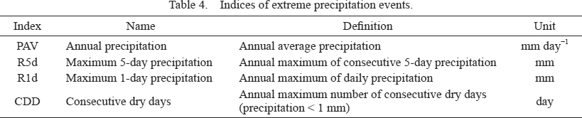
Table 4 shows the definition of extreme precipitation indices used for verification based on Frich et al. (2002). The maximum 5-day precipitation (R5d) is often used to define heavy precipitation events leading to water-related disasters such as inundation and landslides. The maximum 1-day precipitation (R1d) is widely used to define the most extreme precipitation events happening once a year. On the other hand, consecutive dry days (CDD) is an index estimating the possibility of dry conditions and drought. PAV is also included in Table 4 for comparison.
Figure 4 compares the SCC of global distribution of extreme precipitation simulated by CMIP6 models, HighResMIP models and MRI-AGCM models. As for PAV, the AVM of HighResMIP models (blue long thick line) is slightly larger than that of the CMIP6 models (black long thick line). The SCC of MRI-AGCM models (red and purple lines) are larger than most of CMIP6 models (black short line) and most of the HighResMIP models (blue short line).
As for R5d, the SCC of models are generally smaller than that of PAV. The AVM of HighResMIP models (blue long thick line) is slightly larger than that of the CMIP6 models (black long thick line). The SCC of MRI-AGCM models is comparable to or larger than that of CMIP6 models and HighResMIP models.
In the case of R1d, the SCC of models is generally smaller than that of PAV and R5d, suggesting the difficulty to simulate highly heavy rainfall. The AVM of HighResMIP models (blue long thick line) is larger than that of the CMIP6 models (black long thick line). The SCC of MRI-AGCM models is comparable to or larger than that of CMIP6 models and HighResMIP models.
As for CDD, The AVM of HighResMIP models (blue long thick line) is slightly larger than that of the CMIP6 models (black long thick line). The SCC of MRI-AGCM models (red and purple lines) are larger than most of CMIP6 models (black short line) and most of HighResMIP models (blue short line).
In summary, the AVM of HighResMIP models (blue long thick line) is larger than that of the CMIP6 models (black long thick line) for all four precipitation extreme indices. This suggests the advantage of higher horizontal resolution model over lower resolution model in simulating global scale precipitation extreme events. MRI-AGCM models (red and purple lines) perform better than most of other individual models (black and blue short lines) for PAV, R5d, and CDD. This indicates the advantage of very high horizontal resolution models (MRI-AGCM3.2) over lower resolution models in simulating global scale precipitation extreme events.
5. Precipitation over East Asia
MRI-AGCM models have been developed to simulate properly all sorts of meteorological present-day climatology especially over East Asia which is characterized by large precipitation and distinctive rainy season. We have conducted many downscaling studies using MRI-AGCM models as outer boundary conditions of regional climate models over East Asia (Kitoh et al. 2009; Mizuta et al. 2017; Ishii and Mori 2020; Nosaka et al. 2020). Therefore, it is indispensable to validate the ability of MRI-AGCM to simulate precipitation climatology over East Asia.
5.1 Geographical distribution
The rainy season over Japan (the Baiu) starts in the middle of May and terminates in the end of July. Figure 5 compares observed precipitations with simulated precipitations in June. In the GPCPDAY observation (Fig. 5a), precipitation is larger over the Taiwan island, the southern part of China, the East China Sea, and the south of Japan, which corresponds to the Baiu rain band. This rainy zone is also presented in other observations with some differences (Figs. 5b, c). In the APHRODITE observation which is based on rain gauge data over land (Fig. 5d), large precipitation over the southern part of China and the western part of Japan is also presented as a part of the Baiu rain band.

The MME of the CMIP6 models simulates the Baiu rain band, but precipitation is severely underestimated (Fig. 5e). Even the best-performing CMIP6 model also underestimates precipitation of the Baiu rain band (Fig. 5f). The worst-performing CMIP6 model simulates erroneous excessive precipitation to the south of 25°N (Fig. 5g). The underestimation of precipitation over the Baiu rain band (brown color) is obviously recognized in bias distribution (Figs. 5h – j). HighResMIP models also underestimated the precipitation over the Baiu rain band (Figs. 5k – p). MRI-AGCM3.2H (HPD) is selected as the best-performing model of HighResMIP models (Fig. 5l) based on RMSE, but it still underestimates precipitation over the East China Sea and to the south of Japan. MRI-AGCM3.2S (SPD; Figs. S5f, h) also shows a similar distribution to HPD but with less precipitation as compared to HPD to the south of Japan (Fig. S5i; green color).
5.2 Seasonality
Figure 6 shows the seasonality of RMSE over East Asia for all models. In general, RMSEs are larger in summer (June to August) than other seasons. This is due to small SCC in summer (Fig. S6) and negative bias in June (Fig. S7). Also, the low performance of simulating tropical cyclones by models due to insufficient horizontal resolution might lead to large RMSE in summer. The AVMs of the HighResMIP models (blue long thick lines) are equal to or smaller than those of the CMIP6 models (black long thick lines) for all months (Fig. 6). The RMSEs of MRI-AGCM3.2 models (red and purple lines) are equal to or smaller than the AVMs of CMIP6 models (black long thick lines) and HighResMIP models (blue long thick lines) for all months. This suggests the advantage of MRI-AGCM3.2 models over other models in simulating monthly precipitation over East Asia for all months, especially in summer.
5.3 Seasonal march of the rainy season over Japan
Figure 7 depicts the seasonal march of the Japanese rainy season (the Baiu) based on longitudinal averaged pentad precipitation over Japan. In the GPCPDAY observation (Fig. 7a), the Baiu starts in the middle of May at latitude around 25°N. The Baiu migrates northward till the middle of July at latitude around 37°N. Other observations show similar northward migration of the Baiu (Figs. 7b, c). The MME average of CMIP6 models slightly simulates the Baiu (Fig. 7d), but precipitation amount is severely underestimated (Fig. 7g). Although the best-performing CMIP6 model well simulates northward migration of the Baiu (Fig. 7e), precipitation amount is still underestimated (Fig. 7h). The location of the Baiu in the worst-performing CMIP6 model is erroneously shifted to the north of observation (Fig. 7f), resulting in the shortage of precipitation (Fig. 7i). The underestimation of precipitation during the Baiu period by HighResMIP models (Figs. 7j – o) is nearly similar to that by CMIP6 models.

Both HPD (Fig. S8d) and SPD (Fig. S8e) properly simulate northward migration of the Baiu, but they still underestimate precipitation during the Baiu period (Figs. S8f, g). HPD simulates larger precipitation than SPD during the Baiu period (Fig. S8h; green color).
In terms of objective skill scores (Fig. 8), many models show negative bias indicating underestimation of precipitation (horizontal axis in Fig. 8a). The RMSE (vertical axis in Fig. 8a) of the AVM by HighResMIP models (blue square) is slightly smaller than that of CMIP6 models (black square). Also, the magnitude of bias (horizontal axis in Fig. 8a) of the AVM by HighResMIP models (blue square) is slightly smaller than that of the CMIP6 models (black square). MRI-AGCM3.2 models (red and purple crosses) show smaller bias and RMSE than most of other models.
In the Taylor diagram (Fig. 8b), the AVM of HighResMIP models (blue square) is nearer to the observation (green circle) than that of CMIP6 models (black square), indicating the advantage of the HighResMIP models over the CMIP6 models. The performance of MRI-AGCM3.2 models is relatively higher than that of most other models, especially as to SCC.
In summary, the MRI-AGCM3.2 models have advantage over other models in simulating the seasonal march of the rainy season over Japan, although the precipitation amount is still underestimated.
5.4 Comparison with other regions
Figure 9 compares the ability to simulate summer (June–August) precipitation over each square domain with the size of 30 degrees in longitude and latitude. Since spatial standard deviation is generally larger in the tropics than in middle and high latitudes, RMSE tends to be larger in the tropics in most cases. In order to evaluate regional difference of model performance fairly, the RMSE of individual models is normalized by the ratio to spatial standard deviation at each domain. Then, all normalized RMSEs are averaged. Figure 9a shows the average of normalized RMSEs by CMIP6 models over each domain. Since models are forced with observed SST, model performance is generally higher (purple color) over sea than over land. However, normalized RMSEs are relatively large over East Asia. This means the difficulty of simulating summer precipitation over East Asia. The distribution of the average of normalized RMSEs by HighResMIP models (Fig. 9b) is qualitatively similar to CMIP6 models (Fig. 9a). Over East Asia, normalized RMSEs by HighResMIP models are smaller than those by CMIP6 models (Fig. 9c; blue color). This indicates that higher horizontal resolution models perform better in simulating summer precipitation over East Asia than lower horizontal resolution models. This advantage is also evident if model performance is evaluated by SCC for each domain (Fig. S9c). However, this advantage over East Asia is not clear in other seasonal and annual average precipitation (Figure not shown).

6. Skill dependence on horizontal resolution
6.1 Global distribution
Figure 10 shows the relation between the grid size of all 59 models (36 CMIP6 models and 23 HighResMIP models) and model performance. Skill measure is SCC between the observed global distribution of PAV and that simulated by models. Models of smaller grid size (higher horizontal resolution) tend to show higher SCC, therefore grid size and skill are negatively correlated. Note that the vertical axis is reversed in Fig. 10. The correlation coefficient between grid spacing and SCC is −0.441 which is greater than the 99 % significance level. This indicates the advantage of higher horizontal resolution in simulating the global distribution of PAV. The similar advantage of higher horizontal resolution is found for seasonal average precipitation with above the 99 % significance level (Fig. S10; black lines). As for the skill measure of RMSE (Fig. S10; blue lines), the advantage of higher horizontal resolution is smaller than for the skill measure of SCC (Fig. S10; black lines), but the correlation between grid size and RMSE is still above the 95 % significance level for all seasons and annual mean. Although Fig. 3 suggests that the advantage of higher resolution of models (HighResMIP models) over lower resolution models (CMIP6 models) is not clear in terms of AVM (square mark) and MME average (circle mark), correlation statistics between grid size of model and model skill in Fig. 10 has directly revealed the advantage of higher resolution of models.

The similar advantage of higher horizontal resolution model over lower resolution models is also found for simulating extreme precipitation event of R5d and R1d with the skill measure of SCC (Fig. S11).
In the case of Fig. 10, the highest SCC of 0.947 is attained by the ECMWF-IFS-HR with 56 km grid size (Table 2, No. 8, label h), not by the highest horizontal model of MRI-AGCM3.2S (SPD, 21 km, red cross; Table 2, No. 21, label u). This is consistent with previous findings that higher resolution models do not always perform better than lower resolution models (Sperber and Palmer 1996; Kusunoki 2018a; Akinsanola et al. 2020; Bador et al. 2020). The model performance depends on horizontal resolution, but also on implemented physical process such as deep convection scheme (Sperber and Palmer 1996; Kusunoki 2018a). Increasing spatial resolution alone is not sufficient to reduce model errors, and other improvements in physical processes and tuning should be explored (Bador et al. 2020). We will discuss this topic further in the later subsection of 6.4.
6.2 Regionality
The regional dependence of model skill on horizontal resolution is investigated. Figure 11 illustrates whether higher horizontal resolution model perform better than lower resolution model in simulating summer (June–August) precipitation over each domain with the size of 30 degrees in longitude and 30 degrees in latitude. Skill measure is SCC over each domain. Correlation coefficients between grid size and model skill are calculated for all 59 models over each domain. The advantage of higher resolution model is evident over the tropical and northern Pacific Ocean, the Atlantic Ocean, the southern Indian Ocean and East Asia. Similar tendency is also evident for other seasonal and annual average precipitation with some differences (figure not shown). In terms of RMSE, the result is almost similar with weaker relationship between grid size and model skill (figure not shown).
6.3 Seasonality over Japan
The advantage of higher resolution model over lower resolution model around Japan domain (120 – 150°N, 30 – 60°N; black box in Fig. S14a) is larger for summer precipitation than for other seasonal and annual average precipitation (Fig. S12). As for simulating the seasonal march of rainy season over Japan in summer (Figs. 7, 8), higher resolution models tend to perform better than lower resolution model (Fig. S13). These results indicated that higher resolution model is required for better simulation of summer precipitation over Japan.
6.4 Comparison between low resolution and high resolution models in the same institute
In the previous subsections of 6.1 – 6.3, all 59 models are used to evaluate dependence of model skill on horizontal resolution. However, physical processes implemented in models have large difference among institutions. This implies that the effect of difference in physical processes and the effect of difference in horizontal resolution are mixed and are not separated if we use all 59 models in skill-resolution correlation statistics. In HighResMIP, ten institutions submitted simulations conducted with low horizontal model and high resolution model which share the same physical processes and vertical levels. Ten pairs of model names are listed in the left hand side of Table S1. With these ten pairs of models, the relation between skill and horizontal resolution can be purely evaluated without any contamination caused by the effect of difference in physical processes. Table S1 compares the skill of low horizontal model and high resolution model in the same institute for seasonal and annual precipitation over the Japan domain. In the case of skill measure of SCC, seven high resolution models perform better than corresponding low resolution models in the same institute for summer precipitation over the Japan domain. The advantage of high resolution model over low resolution model is not found in other seasonal and annual average precipitation. In the case of RMSE, the advantage of high resolution model is found for summer (80 %) and autumn (70 %).
Figure S14 shows the geographical distribution of the percentage of high resolution model which outperforms corresponding low resolution models in the same institute. Target variable is summer precipitation. The advantage of high resolution model is evident over Asia region, especially over East Asia.
As for the global distribution of seasonal and annual average precipitation, the advantage of higher resolution model over lower resolution model is not clear.
7. Uncertainty of observational data
Observational data with horizontal resolution higher than 1 degree in longitude and latitude have large difference and uncertainties in representing intense precipitation events (Herold et al. 2017; Kitoh and Endo 2019). To evaluate the uncertainty of observational data, we have verified the performance of models against additional precipitation observation datasets of the TRMM and APHRODITE data with the horizontal resolution of 0.25 degree.
7.1 The TRMM data
Figure S15 compares the distribution of extreme precipitation R1d by the TRMM 3B42V7data (0.25 degree), the GPCPDAY V3.2 data (0.50 degree) and the GPCP 1ddV1.3 data (1.0 degree). Because the TRMM data only covers 50°S – 50°N, the target region is limited to 50°S – 50°N in Fig. S15. The distribution of R1d by the GPCPDAY data (global average 77.8 mm) is almost similar to the TRMM data (75.2 mm) with a spatial correlation coefficient of 0.916. In contrast, The GPCP 1dd data severely underestimates R1d precipitation especially over the tropics as compared to higher resolution observations of TRMM data and GPCPDAY data.
Figure 12 compares SCCs verified against the GPCPDAY data and the TRMM data as to the distribution of R1d over 50°S – 50°N. In the case of CMIP6 (black) and HighResMIP (blue) models, model performance verified against the TRMM data is almost comparable to or slightly better than that by the GPCPDAY data. In the case of MRI-AGCM (red and purple), model performance verified against the TRMM data is almost comparable to that by the GPCPDAY data. Small differences of model performance verified against the GPCPDAY data and the TRMM data imply the robustness of verification using the GPCPDAY data.
7.2 The APHRODITE data
We have verified model performance for precipitation over East Asia [110 – 150°N, 20 – 60°N] using the APHRODITE V1901 MA (Monsoon Asia) data which has a high resolution of 0.25 degree (28 km; Table 3), but it covers only land area. RMSE against the APHRODITE MA data (Fig. S16) is qualitatively similar to RMSE against the GPCPDAY data (Fig. 6) in that RMSEs are larger in warmer season, although direct comparison between the two kinds of RMSE is not appropriate because the APHRODITE MA data is limited to land only. Note that vertical axis range in Fig. S16 is smaller than Fig. 6. In Fig. S16, the RMSEs of HighResMIP models in terms of the AVM (blue long line) in warmer season are smaller than that of CMIP6 models (black long line), which is qualitatively similar to Fig. 6. Also, the RMSEs of MRI-AGCM models (red and purple) are smaller or equal to those of CMIP6 models and HighResMIP models in warmer season (Fig. S16), which is also qualitatively similar to Fig. 6.
SCCs by the APHRODITE MA data (Fig. S17) basically represent similar characteristics as that by the GPCPDAY data (Fig S6) regarding smaller skills in warmer seasons, the advantage of HighResMIP models over CMIP6 models and large advantage of MRI-AGCMs.
Biases by the APHRODITE MA data (Fig. S18) tend to show positive value from January to October in contrast to negative biases by the GPCPDAY data from May to December (Fig. S7). In Fig. S18, biases of HighResMIP models in terms of the AVM (blue long line) are smaller than or equal to those of CMIP6 models (black long line) for all months. This advantage of HighResMIP models over CMIP6 models is not so evident in the case of the GPCPDAY data (Fig. S7). The biases of MRI-AGCM3.2 models are nearly comparable to those of CMIP6 models and HighResMIP models in most months (Fig. S18).
In summary, the large similarity between model performance verified against the APHRODITE MA data and the GPCPDAY data for the skill measures of RMSE and SCC enhances the robustness of verification by the GPCPDAY data over the Monsoon Asia region.
7.3 Skill dependence on horizontal resolution
We have evaluated skill dependence on horizontal resolution using the TRMM 3B42V7 data. Figure 13 compares the correlation coefficient between grid size and the SCC of extreme precipitation indices verified against the TRMM data and the GPCPDAY data over the 50°S – 50°N region. The correlation coefficient between grid size and the SCC verified against the TRMM data (red) is almost comparable to that of the GPCPDAY data (black) as for PAV, R5d, and R1d. This gives robustness of the relationship between model grid size and model performance verified against the GPCPDAY data for moderate and intense precipitation.
As for CDD, the relation between grid size and skill is very weak. This is reasonable because CDD often appears as a result of extreme dry condition over large scale region which can be well reproduced even by low resolution models.
8. Conclusions
We have compared the performance of CMIP6 AGCMs, HighResMIP AGCMs, and MRI-AGCM3.2s in simulating precipitation. The performance of HighResMIP models is equal to or slightly better than CMIP6 models in simulating the global distribution of seasonal and annual precipitation. In terms with RMSE and SCC, MRI-AGCMs perform better than CMIP6 models and HighResMIP models in simulating the global distribution of seasonal and annual precipitation. Although most of CMIP6 models and most of HighResMIP models underestimate monthly precipitation in the warmer season (May to August) over East Asia, HighResMIP models perform better than CMIP6 models. The performance of MRI-AGCMs is equal to or better than CMIP6 and HighResMIP models in simulating monthly precipitation over East Asia for all 12 months. Most of CMIP6 and HighResMIP models fail to simulate the northward migration of the rainy zone over Japan resulting in an underestimation of precipitation during the rainy season over Japan. However, MRI-AGCMs perform better than any other models. The advantage of HighResMIP models over CMIP6 models in simulating spatial distribution of summer (June to August) precipitation is more evident over East Asia than in any other region in the globe.
Based on correlation analysis between grid size and model performance using all 59 models, higher horizontal resolution models perform better than lower resolution models in simulating the global distribution of seasonal and annual precipitation. The advantage of higher resolution models over lower resolution models is evident in simulating the seasonal march of the rainy zone over Japan. The advantage of higher resolution model over lower resolution is remarkable in East Asia in simulating summer precipitation compared to other seasons.
Verifications against the TRMM (0.25 degree) data and the APHRODITE MA data (0.25 degree) are basically similar to and consistent with those by the GPCPDAY (0.50 degree). This gives robustness of the results obtained in this paper.
Data Availability Statement
The MRI-AGCM3.2 data are available at the website of the Earth System Grid Federation (ESGF);
https://esgf.llnl.gov/. The CMIP6 AMIP and HighResMIP data are available at the website for the sixth phase of the Coupled Model Intercomparison Project (CMIP6) supplied by the Program for Climate Model Diagnosis and Intercomparison (PCMDI);
https://pcmdi.llnl.gov/CMIP6/.
Supplements
Supplement consists of eighteen figures of Fig. S1 – 18 and one table of Table S1.
Acknowledgments
This work was supported by the advanced studies of climate change projection (SENTAN) Grant Number JPMXD0722680734 funded by the Ministry of Education, Culture, Sports, Science and Technology (MEXT), Japan. We acknowledge the international modeling groups participated to CMIP6, the Earth System Grid Federation (ESGF) which distributes data, and the Working Group on Coupled Modeling (WGCM) Infrastructure Panel which is coordinating and encouraging the development of the infrastructure needed to archive and deliver dataset. We appreciate Drs. H. Kamahori and S. Sugimoto for handling the GPCPDAY data. Thanks are extended to the editor in charge and anonymous reviewers for valuable and constructive comments.
References
- Akinsanola, A. A., G. J. Kooperman, A. G. Pendergrass, W. M. Hannah, and K. A. Reed, 2020: Seasonal representation of extreme precipitation indices over the United States in CMIP6 present-day simulations. Environ. Res. Lett., 15, 094003, doi: 10.1088/1748-9326/ab92c1.
- Alexander, L. V., H. J. Fowler, M. Bador, A. Behrangi, M. G. Donat, R. Dunn, C. Funk, J. Goldie, E. Lewis, M. Rogé, S. I. Seneviratne, and V. Venugopa, 2019: On the use of indices to study extreme precipitation on sub-daily and daily timescales. Environ. Res. Lett., 14, 125008, doi:10.1088/1748-9326/ab51b6.
- Arias, P. A., N. Bellouin, E. Coppola, R. G. Jones, G. Krinner, J. Marotzke, V. Naik, M. D. Palmer, G.-K. Plattner, J. Rogelj, M. Rojas, J. Sillmann, T. Storelvmo, P. W. Thorne, B. Trewin, K. Achuta Rao, B. Adhikary, R. P. Allan, K. Armour, G. Bala, R. Barimalala, S. Berger, J. G. Canadell, C. Cassou, A. Cherchi, W. Collins, W. D. Collins, S. L. Connors, S. Corti, F. Cruz, F. J. Dentener, C. Dereczynski, A. Di Luca, A. Diongue Niang, F. J. Doblas-Reyes, A. Dosio, H. Douville, F. Engelbrecht, V. Eyring, E. Fischer, P. Forster, B. Fox-Kemper, J. S. Fuglestvedt, J. C. Fyfe, N. P. Gillett, L. Goldfarb, I. Gorodetskaya, J. M. Gutiérrez, R. Hamdi, E. Hawkins, H. T. Hewitt, P. Hope, A. S. Islam, C. Jones, D. S. Kaufman, R. E. Kopp, Y. Kosaka, J. Kossin, S. Krakovska, J.-Y. Lee, J. Li, T. Mauritsen, T. K. Maycock, M. Meinshausen, S.-K. Min, P. M. S. Monteiro, T. Ngo-Duc, F. Otto, I. Pinto, A. Pirani, K. Raghavan, R. Ranasinghe, A. C. Ruane, L. Ruiz, J.-B. Sallée, B. H. Samset, S. Sathyendranath, S. I. Seneviratne, A. A. Sörensson, S. Szopa, I. Takayabu, A.-M. Tréguier, B. van den Hurk, R. Vautard, K. von Schuckmann, S. Zaehle, X. Zhang, and K. Zickfeld, 2021: Technical summary. Climate Change 2021: The Physical Science Basis. Contribution of Working Group I to the Sixth Assessment Report of the Intergovernmental Panel on Climate Change. Masson-Delmotte, V., P. Zhai, A. Pirani, S. L. Connors, C. Péan, S. Berger, N. Caud, Y. Chen, L. Goldfarb, M. I. Gomis, M. Huang, K. Leitzell, E. Lonnoy, J. B. R. Matthews, T. K. Maycock, T. Waterfield, O. Yelekçi, R. Yu, and B. Zhou (eds.), Cambridge University Press, 33–144.
- Bador, M., L. V. Alexander, S. Contractor, and R. Roca, 2020a: Diverse estimates of annual maxima daily precipitation in 22 state-of-the-art quasi-global land observation datasets Environ. Res. Lett., 15, 035005, doi: 10.1088/1748-9326/ab6a22.
- Bador, M., J. Boé, L. Terray, L. V. Alexander, A. Baker, A. Bellucci, R. Haarsma, T. Koenigk, M.-P. Moine, K. Lohmann, D. A. Putrasahan, C. Roberts, M. Roberts, E. Scoccimarro, R. Schiemann, J. Seddon, R. Senan, S. Valcke, and B. Vanniere, 2020b: Impact of higher spatial atmospheric resolution on precipitation extremes over land in global climate models. J. Geophys. Res.: Atmos., 125, e2019JD032184, doi: 10.1029/2019JD032184.
- Chen, C.-A., H.-H. Hsu, C.-C. Hong, P.-G. Chiu, C.-Y. Tu, S.-J. Lin, and A. Kitoh, 2019: Seasonal precipitation change in the western North Pacific and East Asia under global warming in two high-resolution AGCMs. Climate Dyn., 53, 5583–5605.
- Chen, C.-A., H.-H. Hsu, and H.-C. Liang, 2021: Evaluation and comparison of CMIP6 and CMIP5 model performance in simulating the seasonal extreme precipitation in the western North Pacific and East Asia. Wea. Climate Extremes, 31, 100303, doi: 10.1016/j.wace.2021.100303.
- Chen, D., M. Rojas, B. H. Samset, K. Cobb, A. Diongue Niang, P. Edwards, S. Emori, S. H. Faria, E. Hawkins, P. Hope, P. Huybrechts, M. Meinshausen, S. K. Mustafa, G.-K. Plattner, and A.-M. Tréguier, 2021: Framing, context, and methods. Climate Change 2021: The Physical Science Basis. Contribution of Working Group I to the Sixth Assessment Report of the Intergovernmental Panel on Climate Change. Masson-Delmotte, V., P. Zhai, A. Pirani, S. L. Connors, C. Péan, S. Berger, N. Caud, Y. Chen, L. Goldfarb, M. I. Gomis, M. Huang, K. Leitzell, E. Lonnoy, J. B. R. Matthews, T. K. Maycock, T. Waterfield, O. Yelekçi, R. Yu, and B. Zhou (eds.), Cambridge University Press, 147–286.
- Dong, T., and W. Dong, 2021: Evaluation of extreme precipitation over Asia in CMIP6 models. Climate Dyn., 57, 1751–1769.
- Endo, H., A. Kitoh, T. Ose, R. Mizuta, and S. Kusunoki, 2012: Future changes and uncertainties in Asian precipitation simulated by multiphysics and multi–sea surface temperature ensemble experiments with highresolution Meteorological Research Institute atmospheric general circulation models (MRI-AGCMs). J. Geophys. Res., 117, D16118, doi: 10.1029/2012JD017874.
- Eyring, V., S. Bony, G. A. Meehl, C. A. Senior, B. Stevens, R. J. Stouffer, and K. E. Taylor, 2016: Overview of the Coupled Model Intercomparison Project Phase 6 (CMIP6) experimental design and organization. Geosci. Model Dev., 9, 1937–1958.
- Eyring, V., N. P. Gillett, K. M. Achuta Rao, R. Barimalala, M. Barreiro Parrillo, N. Bellouin, C. Cassou, P. J. Durack, Y. Kosaka, S. McGregor, S. Min, O. Morgenstern, and Y. Sun, 2021: Human influence on the climate system. Climate Change 2021: The Physical Science Basis. Contribution of Working Group I to the Sixth Assessment Report of the Intergovernmental Panel on Climate Change. Masson-Delmotte, V., P. Zhai, A. Pirani, S. L. Connors, C. Péan, S. Berger, N. Caud, Y. Chen, L. Goldfarb, M. I. Gomis, M. Huang, K. Leitzell, E. Lonnoy, J. B. R. Matthews, T. K. Maycock, T. Waterfield, O. Yelekçi, R. Yu, and B. Zhou (eds.), Cambridge University Press, 423–552.
- Fábrega, J., T. Nakaegawa, R. Pinzón, K. Nakayama, O. Arakawa, and SOUSEI Theme-C Modeling Group, 2013: Hydroclimate projections for Panama in the 21st Century. Hydrol. Res. Lett., 7, 23–29.
- Frich, P., L. V. Alexander, P. Della-Marta, B. Gleason, M. Haylock, A. M. G. Klein Tank, and T. Peterson, 2002: Observed coherent changes in climatic extremes during the second half of the twentieth century. Climate Res., 19, 193–212.
- Gleckler, P. J., K. E. Taylor, and C. Doutriaux, 2008: Performance metrics for climate models. J. Geophys. Res., 113, D06104, doi: 10.1029/2007JD008972.
- Haarsma, R. J., M. J. Roberts, P. L. Vidale, C. A. Senior, A. Bellucci, Q. Bao, P. Chang, S. Corti, N. S. Fučkar, V. Guemas, J. von Hardenberg, W. Hazeleger, C. Kodama, T. Koenigk, L. R. Leung, J. Lu, J.-J. Luo, J. Mao, M. S. Mizielinski, R. Mizuta, P. Nobre, M. Satoh, E. Scoccimarro, T. Semmler, J. Small, and J.-S. von Storch, 2016: High resolution model intercomparison project (HighResMIP v1.0) for CMIP6. Geosci. Model Dev., 9, 4185–4208.
- Herold, N., A. Behrangi, and L. V. Alexander, 2017: Large uncertainties in observed daily precipitation extremes over land. J. Geophys. Res.: Atmos., 122, 668–681.
- Huffman, G. J., R. F. Adler, M. M. Morrissey, D. T. Bolvin, S. Curtis, R. Joyce, B. McGavock, and J. Susskind, 2001: Global precipitation at one-degree daily resolution from multisatellite observations. J. Hydrometeor., 2, 36–50.
- Huffman, G. J., D. T. Bolvin, E. J. Nelkin, D. B. Wolff, R. F. Adler, G. Gu, Y. Hong, K. P. Bowman, and E. F. Stocker, 2007: The TRMM multisatellite precipitation analysis (TMPA): Quasi-global, multiyear, combined-sensor precipitation estimates at fine scales. J. Hydrometeor., 8, 38–55.
- Huffman, G. J., D. T. Bolvin, D. Braithwaite, K. Hsu, R. Joyce, and P. Xie, 2015: NASA global precipitation measurement (GPM) integrated multi-satellite retrievals for GPM (I-MERG). Algorithm Theoretical Basis Doc. (ATBD), version 4.5, Greenbelt, MD, 26 pp. [Available at http://pmm.nasa.gov/sites/default/files/document_files/IMERG_ATBD_V4.5.pdf.]
- Huffman, G. J., A. Behrangi, D. T. Bolvin, E. J. Nelkin, 2022: GPCP Version 3.2 Daily Precipitation Data Set (GPCPDAY). GES DISC, Greenbelt, MD, doi: 10.5067/MEASURES/GPCP/DATA305. (Accessed 25 October 2023)
- IPCC, 2021: Climate Change 2021: The Physical Science Basis. Contribution of Working Group I to the Sixth Assessment Report of the Intergovernmental Panel on Climate Change. Masson-Delmotte, V., P. Zhai, A. Pirani, S. L. Connors, C. Péan, S. Berger, N. Caud, Y. Chen, L. Goldfarb, M. I. Gomis, M. Huang, K. Leitzell, E. Lonnoy, J. B. R. Matthews, T. K. Maycock, T. Waterfield, O. Yelekçi, R. Yu, and B. Zhou (eds.), Cambridge University Press, doi: 10.1017/9781009157896.
- Ishii, M., and N. Mori, 2020: d4PDF: Large-ensemble and high-resolution climate simulations for global warming risk assessment. Prog. Earth Planet. Sci., 7, 58, doi: 10.1186/s40645-020-00367-7.
- Kamiguchi, K., A. Kitoh, T. Uchiyama, R. Mizuta, and A. Noda, 2006: Changes in precipitation-based extremes indices due to global warming projected by a global 20-km-mesh atmospheric model. SOLA, 2, 64–67.
- Kang, I. S., K. Jin, B. Wang, K. M. Lau, J. Shukla, V. Krishnamurthy, S. D. Schubert, D. E. Wailser, W. F. Stern, A. Kitoh, G. A. Meehl, M. Kanamitsu, V. Y. Galin, V. Satyan, C. K. Park, and Y. Liu, 2002: Intercomparison of the climatological variations of Asian summer monsoon precipitation simulated by 10 GCMs. Climate Dyn., 19, 383–395.
- Kitoh, A., and S. Kusunoki, 2008: East Asian summer monsoon simulation by a 20-km mesh AGCM. Climate Dyn., 31, 389–401.
- Kitoh, A., and H. Endo, 2016: Changes in precipitation extremes projected by a 20-km mesh global atmospheric model. Wea. Climate Extremes, 11, 41–52.
- Kitoh, A., and H. Endo, 2019: Future changes in precipitation extremes associated with tropical cyclones projected by large-ensemble simulations. J. Meteor. Soc. Japan, 97, 141–152.
- Kitoh, A., T. Ose, K. Kurihara, S. Kusunoki, M. Sugi, and KAKUSHIN Team-3 Modeling Group, 2009: Projection of changes in future weather extremes using super-high-resolution global and regional atmospheric models in the KAKUSHIN Program: Results of preliminary experiments. Hydrol. Res. Lett., 3, 49–53.
- Kusunoki, S., 2017: Future changes in global precipitation projected by the atmospheric model MRI-AGCM3.2H with a 60-km size. Atmosphere, 8, 93, doi: 10.3390/atmos8050093.
- Kusunoki, S., 2018a: Is the global atmospheric model MRI-AGCM3.2 better than the CMIP5 atmospheric models in simulating precipitation over East Asia? Climate Dyn., 51, 4489–4510.
- Kusunoki, S., 2018b: Future changes in precipitation over East Asia projected by the global atmospheric model MRI-AGCM3.2. Climate Dyn., 51, 4601–4617.
- Kusunoki, S., 2018c: How will the onset and retreat of rainy season over East Asia change in future? Atmos. Sci. Lett., 19, e824, doi: 10.1002/asl.824.
- Kusunoki, S., and R. Mizuta, 2008: Future changes in the Baiu rain band projected by a 20-km mesh global atmospheric model: Sea surface temperature dependence. SOLA, 4, 85–88.
- Kusunoki, S., and R. Mizuta, 2012: Comparison of near future (2015–2039) changes in the East Asian rain band with future (2075–2099) changes projected by global atmospheric models with 20-km and 60-km grid size. SOLA, 8, 73–76.
- Kusunoki, S., and R. Mizuta, 2013: Changes in precipitation intensity over East Asia during the 20th and 21st centuries simulated by a global atmospheric model with a 60 km grid size. J. Geophys. Res.: Atmos., 118, 11007–11016.
- Kusunoki, S., and O. Arakawa, 2015: Are CMIP5 models better than CMIP3 models in simulating precipitation over East Asia? J. Climate, 28, 5601–5621.
- Kusunoki, S., and R. Mizuta, 2021: Future changes in rainy season over East Asia projected by massive ensemble simulations with a high-resolution global atmospheric model. J. Meteor. Soc. Japan, 99, 79–100.
- Kusunoki, S., M. Sugi, A. Kitoh, C. Kobayashi, and K. Takano, 2001: Atmospheric seasonal predictability experiments by the JMA AGCM. J. Meteor. Soc. Japan, 79, 1183–1206.
- Kusunoki, S., J. Yoshimura, H. Yoshimura, A. Noda, K. Oouchi, and R. Mizuta, 2006: Change of Baiu rain band in global warming projection by an atmospheric general circulation model with a 20-km grid size. J. Meteor. Soc. Japan, 84, 581–611.
- Kusunoki, S., R. Mizuta, and M. Matsueda, 2011: Future changes in the East Asian rain band projected by global atmospheric models with 20-km and 60-km grid size. Climate Dyn., 37, 2481–2493.
- Kusunoki, S., T. Nakaegawa, R. Pinzón, J. E. Sanchez-Galan and J. R. Fábrega, 2019: Future precipitation changes over Panama projected with the atmospheric global model MRI-AGCM3.2. Climate Dyn., 53, 5019–5034.
- Lambert, S. J., and G. J. Boer, 2001: CMIP1 evaluation and intercomparison of coupled climate models. Climate Dyn., 17, 83–106.
- Lau, K. M., and S. Yang, 1996: Seasonal variation, abrupt transition, and intraseasonal variability associated with the Asian summer monsoon in the GLA GCM. J. Climate, 9, 965–985.
- Lau, K.-M., J. H. Kim, and Y. Sud, 1996: Intercomparison of hydrologic processes in AMIP GCMs. Bull. Amer. Meteor. Soc., 77, 2209–2227.
- Liang, X.-Z., W.-C. Wang, and A. N. Samel, 2001: Biases in AMIP model simulations of the east China monsoon system. Climate Dyn., 17, 291–304.
- Liang, J., M. L. Tan, M. Hawcroft, J. L. Catto, K. I. Hodges, and J. M. Haywood, 2022: Monsoonal precipitation over Peninsular Malaysia in the CMIP6 HighResMIP experiments: The role of model resolution. Climate Dyn., 58, 2783–2805.
- Lui, Y. S., C.-Y. Tam, and N.-C. Lau, 2019: Future changes in Asian summer monsoon precipitation extremes as inferred from 20-km AGCM simulations. Climate Dyn., 52, 1443–1459.
- Martínez, M. M., T. Nakaegawa, R. Pinzón, S. Kusunoki, R. Gordón, and J. E. Sanchez-Galan, 2020: Using a statistical crop model to predict maize yield by the end-of-century for the Azuero region in Panama. Atmosphere, 11, 1097, doi: 10.3390/atmos11101097.
- Masunaga, H., M. Schröder, F. A. Furuzawa, C. Kummerow, E. Rustemeier, and U. Schneider, 2019: Inter-product biases in global precipitation extremes. Environ. Res. Lett., 14, 125016, doi: 10.1088/1748-9326/ab5da9.
- Mizuta, R., H. Yoshimura, H. Muraklami, M. Matsueda, H. Endo, T. Ose, K. Kamiguchi, M. Hosaka, M. Sugi, S. Yukimoto, S. Kusunoki, and A. Kitoh, 2012: Climate simulations using MRI-AGCM3.2 with 20-km grid. J. Meteor. Soc. Japan, 90A, 233–258.
- Mizuta, R., A. Murata, M. Ishii, H. Shiogama, K. Hibino, N. Mori, O. Arakawa, Y. Imada, K. Yoshida, T. Aoyagi, H. Kawase, M. Mori, Y. Okada, T. Shimura, T. Nagatomo, M. Ikeda, H. Endo, M. Nosaka, M. Arai, C. Takahashi, K. Tanaka, T. Takemi, Y. Tachikawa, K. Temur, Y. Kamae, M. Watanabe, H. Sasaki, A. Kitoh, I. Takayabu, E. Nakakita, and M. Kimoto, 2017: Over 5,000 years of ensemble future climate simulations by 60-km global and 20-km regional atmospheric models. Bull. Amer. Meteor. Soc., 98, 1383–1398.
- Nakaegawa, T., A. Kitoh, Y. Ishizaki, S. Kusunoki, and H. Murakami, 2014a: Caribbean low-level jets and accompanying moisture fluxes in a global warming climate projected with CMIP3 multi-model ensemble and fine-mesh atmospheric general circulation models. Int. J. Climatol., 34, 964–977.
- Nakaegawa, T., A. Kitoh, S. Kusunoki, H. Murakami, and O. Arakawa, 2014b: Hydroclimate changes over Central America and the Caribbean in a global warming climate projected with 20-km and 60-km mesh MRI atmospheric general circulation models. Pap. Meteor. Geophys., 65, 15–33.
- Nakaegawa, T., A. Kitoh, H. Murakami, and S. Kusunoki, 2014c: Annual maximum 5-day rainfall total and maximum number of consecutive dry days over Central America and the Caribbean in the late twenty-first century projected by an atmospheric general circulation model with three different horizontal resolutions. Theor. Appl. Climatol., 116, 155–168.
- Nosaka, M., M. Ishii, H. Shiogama, R. Mizuta, A. Murata, H. Kawase, and H. Sasaki, 2020: Scalability of future climate changes across Japan examined with large-ensemble simulations at +1.5 K, +2 K, and +4 K global warming levels. Prog. Earth Planet. Sci., 7, 27, doi: 10.1186/s40645-020-00341-3.
- Okada, Y., T. Takemi, H. Ishikawa, S. Kusunoki, and R. Mizuta, 2017: Future changes in atmospheric conditions for the seasonal evolution of the Baiu as revealed from projected AGCM experiments. J. Meteor. Soc. Japan, 95, 239–260.
- Pinzón, R., K. Hibino, I. Takayabu, and T. Nakaegawa, 2017: Virtually experiencing future climate changes in Central America with MRI-AGCM: Climate analogues study. Hydrol. Res. Lett., 11, 106–113.
- Randall, D. A., R. A. Wood, S. Bony, R. Colman, T. Fichefet, J. Fyfe, V. Kattsov, A. Pitman, J. Shukla, J. Srinivasan, R. J. Stouffer, A. Sumi, and K. E. Taylor, 2007: Climate models and their evaluation. Climate Change 2007: The Physical Science Basis. Contribution of Working Group I to the Fourth Assessment Report of the Intergovernmental Panel on Climate Change. Solomon, S., D. Qin, M. Manning, Z. Chen, M. Marquis, K. B. Averyt, M. Tignor, and H. L. Miller (eds.), Cambridge University Press.
- Rayner, N. A., D. E. Parker, E. B. Horton, C. K. Folland, L. V. Alexander, D. P. Rowell, E. C. Kent, and A. Kaplan, 2003: Global analyses of sea surface temperature, sea ice, and night marine air temperature since the late nineteenth century. J. Geophys. Res., 108, 4407, doi: 10.1029/2002JD002670.
- Reichler, T., and J. Kim, 2008: How well do coupled models simulate today’s climate? Bull. Amer. Meteor. Soc., 89, 303–312.
- Sillmann, J., V. V. Kharin, X. Zhang, F. W. Zwiers, and D. Bronaugh, 2013: Climate extremes indices in the CMIP5 multimodel ensemble: Part 1. Model evaluation in the present climate. J. Geophys. Res.: Atmos., 118, 1716–1733.
- Skofronick-Jackson, G., W. A. Petersen, W. Berg, C. Kidd, E. F. Stocker, D. B. Kirschbaum, R. Kakar, S. A. Braun, G. J. Huffman, T. Iguchi, P. E. Kirstetter, C. Kummerow, R. Meneghini, R. Oki, W. S. Olson, Y. N. Takayabu, K. Furukawa, and T. Wilheit, 2017: The global precipitation measurement (GPM) mission for science and society. Bull. Amer. Meteor. Soc., 98, 1679–1695.
- Sperber, K. R., and T. N. Palmer, 1996: Interannual tropical rainfall variability in general circulation model simulations associated with the Atmospheric Model Intercomparison Project. J. Climate., 9, 2727–2750.
- Sperber, K. R., H. Annamalai, I.-S. Kang, A. Kitoh, A. Moise, A. Turner, B. Wang, and T. Zhou, 2013: The Asian summer monsoon: An intercomparison of CMIP5 vs. CMIP3 simulations of the late 20th century. Climate Dyn., 41, 2711–2744.
- Srivastava, A., R. Grotjahn, and P. A. Ullrich, 2020: Evaluation of historical CMIP6 model simulations of extreme precipitation over contiguous US regions. Wea. Climate Extremes, 29, 100268, doi: 10.1016/j.wace.2020.100268.
- Tan, M. L., J. Liang, M. Hawcroft, J. M. Haywood, F. Zhang, R. Rainis, and W. R. Ismail, 2021: Resolution dependence of regional hydro-climatic projection: A case-study for the Johor River basin, Malaysia. Water, 13, 3158, doi: 10.3390/w13223158.
- Taylor, K. E., 2001: Summarizing multiple aspects of model performance in a single diagram. J. Geophys. Res., 106, 7183–7192.
- Taylor, K. E., R. J. Stouffer, and G. A. Meehl, 2012: An overview of CMIP5 and the experiment design. Bull. Amer. Meteor. Soc., 93, 485–498.
- Tiedtke, M., 1989: A comprehensive mass flux scheme for cumulus parameterization in large-scale models. Mon. Wea. Rev., 117, 1779–1800.
- Yatagai, A., O. Arakawa, K. Kamiguchi, H. Kawamoto, M. I. Nodzu, and A. Hamada, 2009: A 44-year daily gridded precipitation dataset for Asia based on a dense network of rain gauges. SOLA, 5, 137–140.
- Yatagai, A., K. Kamiguchi, O. Arakawa, A. Hamada, N. Yasutomi, and A. Kitoh, 2012: APHRODITE: Constructing a long-term daily gridded precipitation dataset for Asia based on a dense network of rain gauges. Bull. Amer. Meteor. Soc., 93, 1401–1415.
- Yoshimura, H., R. Mizuta, and H. Murakami, 2015: A spectral cumulus parameterization scheme interpolating between two convective updrafts with semi-Lagrangian calculation of transport by compensatory subsidence. Mon. Wea. Rev., 143, 597–621.


