Improvement of Two-Hour-Ahead QPF Using Blending Technique with Spatial Maximum Filter for Tolerating Forecast Displacement Errors and Water Vapor Lidar Assimilation

Abstract

Disasters caused by heavy rainfall associated with quasi-stationary line-shaped mesoscale convective systems (MCSs) frequently occur in Japan. Thus, highly accurate quantitative precipitation forecast (QPF) information that contributes to decision-making by municipalities to issue evacuation orders is necessary. To this end, we developed a blending forecasting system (BFS) for predicting heavy rainfall associated with MCSs. The BFS blends 1-h observed rainfall and forecasts of extrapolation-based nowcasting (EXT) in the first hour and numerical weather prediction (NWP) in the second hour, predicting 3-h accumulated rainfall (P3h) and its return period (RP) of up to 2 h ahead with a higher horizontal resolution (1 km) and higher-frequency updates (every 10 min) compared to the current operational systems. A blending technique with a spatial maximum filter for tolerating forecast displacement errors (BLEDE) was applied to the predicted rainfall of EXT and NWP. To improve the accuracy of the NWP, vertical profiles of water vapor obtained with two water vapor lidars (WVLs) were assimilated into the NWP. This combination predicted rare heavy rainfall with an RP of more than 10 years in the same city where flooding occurred for a heavy rainfall event associated with quasi-stationary line-shaped MCSs in southern Kyushu on 10 July 2021. The BFS yielded such forecast information 40 min earlier than the existing warning information, indicating the potential for providing a longer lead time for evacuation. The improvement in forecast accuracy was due to both BLEDE and WVL data assimilation (WVL-DA); however, the contribution of BLEDE was more than five times that of WVL-DA in terms of predicting the P3h for the threshold of 80 mm. Additionally, the sensitivity of the predicted rainfall to the background error covariance matrix in WVL-DA is also discussed.

1. Introduction

Disasters caused by heavy rainfall associated with quasi-stationary line-shaped mesoscale convective systems (QSLS-MCSs) frequently occur in Japan. Such events include those in Hiroshima in August 2014 (Kato et al. 2016; Oizumi et al. 2020), northern Kyushu in July 2017 (Kato et al. 2018), and southern Kyushu in July 2020 (Hirockawa et al. 2020a). Such QSLS-MCSs and associated band-shaped heavy rainfall areas with lengths of 50 – 300 km and widths of 20 – 50 km are typically referred to as “senjo-kousuitai” in Japan (Kato 2020). As municipalities issue evacuation orders during heavy rainfall, highly accurate quantitative precipitation forecast (QPF) information that contributes to decision-making by municipalities to issue evacuation orders is crucial at the municipality scale (∼ 15 km).

For heavy rainfall associated with QSLS-MCSs, it is important to predict the accumulated rainfall with high accuracy as it is more closely related to disasters than the instantaneous rainfall intensity. For instance, 3-h accumulated rainfall (P3h) is used as one of the criteria for “information on significant heavy rainfall” issued by the Japan Meteorological Agency (JMA; Japan Meterological Agency 2022).

Forecasting of such accumulated rainfall can be performed using blending forecasting (BF; Sun et al. 2014), which involves the use of extrapolation-based nowcasting (EXT) at the beginning of forecasting and gradually replaces it with numerical weather prediction (NWP). The forecast accuracy of NWP can be superior to that of EXT with increasing forecast time (FT) owing to the potential of NWP to predict the development and decay of rainfall. Hatsuzuka et al. (2022) statistically evaluated the prediction accuracy of P3h associated with QSLS-MCS using the JMA’s immediate, very short-range forecast of precipitation (VSRF), which is a BF. The results showed that the VSRF is useful up to FT = 2 h (P3h at FT = 2 h was the sum of 1-h accumulated rainfall (P1h) of observation and 2-h accumulated rainfall of VSRF) even at the original resolution (1 km) for heavy rainfall areas of ≥ 80 mm (3 h)⁻¹, but it does not provide useful prediction on and after FT = 3 h, even if displacement errors at municipal or larger scales (15 – 31 km) were tolerated. The study also demonstrated that the VSRF exhibits reduced skillfulness in the formation stage of QSLS-MCSs at shorter FTs (1 – 2 h), a shortcoming attributed to the limitations of the extrapolation forecasts. This finding underscores the necessity to improve forecast accuracy during the formation stage of QSLS-MCSs, as it can significantly influence the timing of warning issuance and decision-making processes related to evacuation. This study focuses on the prediction of rainfall in the formation stage of QSLS-MCSs, which is difficult but vital for the protection of the population and property.

Three major problems are associated with blending prediction for forecasting heavy rainfall associated with MCS at the very short-range FT scale (several hours). The first problem is the underestimation of rainfall owing to displacement errors of forecasts (Hwang et al. 2015; Fukuhara et al. 2019). If the two forecasting methods (i.e., EXT and NWP) for the blending prediction have different forecast displacement errors, the peak of accumulated rainfall is underestimated by simply blending the two forecasts using only the temporal weight (Hwang et al. 2015). This may result in the failure to predict the potential disaster resulting from heavy rainfall. Therefore, a blending technique for tolerating forecast displacement errors (BLEDE) is required to modify rainfall distribution by considering the displacement errors of the two types of forecasts (Shimizu et al. 2020; Kato et al. 2021). The second problem is the insufficient accuracy of NWP at the very short range because of spin-up issues (Sun et al. 2014; Japan Meteorological Agency 2019). This problem can be alleviated by using observation data and EXT rather than NWP for calculating P3h at the beginning of the FT. The third problem, which is also related to the insufficient accuracy of NWP used in blending methods, is the insufficient observation of low-level moisture for the assimilation with NWP. Numerous numerical simulations have reproduced moist low-level inflows into MCSs (Kato and Goda 2001; Xu et al. 2012; Luo et al. 2014; Peters and Schumacher 2015; Jeong et al. 2016; Hirota et al. 2016; Zhang et al. 2019; Kawano and Kawamura 2020). Additionally, statistical analyses of severe precipitation events associated with MCSs have revealed that low-level moist inflows are frequently involved (Unuma and Takemi 2016; Araki et al. 2021). According to these simulations, observations, and analyses, moist low-level inflows are a typical characteristic of MCSs and are crucial for comprehending how they form and are maintained. Improved vertical representations of low-level moist inflows in the numerical models can also significantly improve the forecasts of the localized heavy rainfall associated with MCSs (Kato et al. 2003; Schumacher 2015; Peters et al. 2017; Lee et al. 2018). The assimilation of water vapor vertical profiles measured by a water vapor lidar (WVL) reportedly has a positive impact on predicting heavy rainfall associated with an MCS based on an Observing System Simulation Experiment (Yoshida et al. 2020), a real case forecast experiment associated with an MCS on a warm front (Yoshida et al. 2022), and an MCS on a stationary front (Yoshida et al. 2024).

Our group has been developing a blending forecasting system (BFS) for heavy rainfall associated with MCSs (Shimizu et al. 2020). The system provides a higher-resolution (horizontal grid spacing Δx = 1 km) and higher-frequency update (every 10 min) compared to the current operational systems. A QPF of up to 2 h ahead can support the decision-making process of municipalities in issuing evacuation orders (Shimizu et al. 2020). A unique feature of the BFS is that it also provides a return period (RP) of the accumulated rainfall. The rainfall RP is an indicator of the rarity of heavy rainfall in a given area and is widely used in risk analyses. The rainfall RP may be more useful than simple accumulated rainfall in the decision-making process of municipalities (Hirano 2019). The BFS combines the blending of observation data, EXT, and NWP with a BLEDE technique alongside the assimilation of various water vapor observation data, and it is currently being applied using data from Kyushu. Shimizu et al. (2020) previously demonstrated the effectiveness of the BFS in the formation stage of QSLS-MCSs for heavy rainfall in Saga Prefecture on 28 August 2019. However, they have not investigated the contribution of BLEDE in the blending prediction. Moreover, the assimilation impact of water vapor observation data has remained unclear because our water vapor observation instruments had not yet been installed in Kyushu at the time of the study in 2019. In 2020, two WVLs were installed in Kyushu, enabling real-time assimilation of vertical profiles of water vapor.

On 10 July 2021, a back-building (BB) type of QSLS-MCS involving a band-shaped heavy precipitation area, a so-called senjo-kousuitai, occurred in Kagoshima Prefecture. The JMA announced “information on significant heavy rainfall,” which indicates the occurrence of senjo-kousuitai, in the Satsuma region of Kagoshima Prefecture in Kyushu (Japan Meteorological Agency 2021). Rivers overflowed in the Kagoshima Prefecture, causing substantial damage, such as inundation above the floor level of houses (Kagoshima Prefecture 2022). In this study, we provided the details of the BFS (Section 2: Data and method) and elucidated the contribution of the BLEDE and WVL data assimilation (WVL-DA) to the QPF (Section 3: Results) of this event. The sensitivity of the predicted rainfall to the background error covariance matrix (B) in WVL-DA is also discussed (Section 4: Discussion). This is the first study to demonstrate the effectiveness of BLEDE and WVL-DA for 2-h-ahead QPF of heavy rainfall associated with QSLS-MCSs.

2. Data and methods

2.1 BFS with the BLEDE

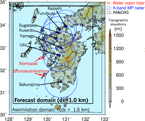
The BFS is a unique system that blends P1h of observations, EXT, and NWP with the BLEDE to predict P3h at FT = 2 h. For the past 1 h of P3h of blending prediction (FT = −1 – 0 h), we used the observed rainfall from X-band multiparameter (X-MP) radars of the eXtended RAdar Information Network (XRAIN; Godo et al. 2014) operated by Japan’s Ministry of Land, Infrastructure, Transport and Tourism. To resolve the spin-up problem of NWP, the blending prediction applies P1h from FT = 0 – 1 h of the JMA high-resolution precipitation nowcasts (Kigawa 2014; Kato et al. 2017a) as EXT for FT = 0 – 1 h of the BF. The P1h from FT = 1 – 2 h of Cloud Resolving Storm Simulator (CReSS; Tsuboki and Sakakibara 2002) was used as the NWP model with the DA for FT = 1 – 2 h of the BF. The NWP settings were nearly identical to those used by Kato et al. (2018), who investigated the predictability of the July 2017 northern Kyushu heavy rainfall with the same horizontal grid spacing of Δx = 1 km. The NWP calculation domain (thick box in Fig. 1) covered the Kyushu area with Δx = 1 km, which was slightly narrower than that from the calculation domain of Kato et al. (2018). The NWP calculation domain was the same as the blending prediction domain. The model top was 20.6 km, a height that exceeds the 17.2 km used by Kato et al. (2018). Horizontal and vertical grid points of NWP were 464 × 480 × 50.

Fig. 1

Forecast and assimilation domain as well as location of instruments used for data assimilation. Red stars represent the locations of water vapor lidars [WVLs: Nomozaki (Na) and Shimokoshikishima (Ko)]. Blue circles represent the observation range (80 km) of X-band MP radars (Sakurajima, Uki, Yamaga, Kusenbu, Sugadake, Furutsuki, and Kazashi) of XRAIN. White squares represent the locations of surface anemometers of the Automated Meteorological Data Acquisition System (AMeDAS) of JMA. Different colors represent topographic elevations.

For the forecasted P1h of EXT and NWP, the BLEDE was applied to alleviate the underestimation of the peak value of accumulated rainfall for the BF (Shimizu et al. 2020; Kato et al. 2021). For BLEDE, a spatial maximum filter was applied to replace the rainfall at each grid point with the maximum value within the L × L km² around the grid point. Note that L is preferably determined based on a statistical scale of displacement error for each forecast. The spatial maximum filter enabled the expansion of the heavy rainfall area of each forecast. This allowed for predicting the peak of the accumulated rainfall in the BF. The L was set to 7 km for EXT and 11 km for NWP for the BFS based on the accuracy of each prediction for the northern Kyushu heavy rainfall in July 2017 (Shimizu et al. 2020). Note that the BF product of P3h is created by simply adding together the P1h of the observation, the P1h of EXT with BLEDE, and the P1h of NWP with BLEDE. The temporal weight for blending may be advanced in the future.

2.2 CReSS-3DVAR

The initial values of the NWP were estimated from the three-dimensional variational method (3DVAR) with incremental analysis updates (IAU) by using the CReSS (Shimose et al. 2017). Note that the analysis of the 3DVAR with IAU using the CReSS (CReSS-3DVAR) was conducted for a slightly wider region compared to that of the NWP (see the solid box in Fig. 1); it used Δx = 1.5 km with horizontal and vertical grid points of 288 × 352 × 50 and produced analysis values every 10 min. The forecast values at FT = 1h of the latest JMA Local Forecast Model (LFM; Japan Meteorological Agency 2019) data available in realtime were used as the initial condition of the first guess of the CReSS-3DVAR.

In the CReSS-3DVAR, analysis-forecast cycling assimilation is performed in two main steps. First, analysis values are created using background forecast values of the CReSS and observation data by employing 3DVAR with IAU. Then, background forecasts of the CReSS are conducted using the analysis values as the initial condition. Specifically, 1-h interval LFM data are used as the initial condition of the first guess to carry out analysis-forecast cycles up to 90 min. To incorporate observations from multiple times into the analysis values, the analysis values output every 10 min from 40 – 90 min are used as initial values for NWP used in blending prediction. The WVL data, described in detail in the next subsection, are available every 15 min and are assimilated every 10 min or 20 min using the 3DVAR. Specifically, in the real-time analysis-forecast cycling DA, WVL data at 00, 15, 30, 45, 60, and 75 min are used in the 3DVAR to create analysis values at 10, 20, 40, 50, 70, and 80 min. For instance, consider the case of conducting an NWP with a start time of 1300. In this scenario, the forecast value at 1200, which is 1 h ahead of the LFM forecast with a start time of 1100, becomes the initial value for the analysis-forecast assimilation cycle by CReSS-3DVAR. The analysis value at 1300, 1 h after the start of the assimilation cycle, is utilized as the initial value for the NWP. In this context, four WVL profiles at 1200, 1215, 1230, and 1245 are assimilated through the cycling process.

The following observation data were assimilated in the CReSS-3DVAR: the vertical profiles of water vapor mixing ratio (q_v) from WVLs installed at Nomozaki, Nagasaki Prefecture (hereafter referred to as Na lidar) and Shimokoshikishima, Kagoshima Prefecture (hereafter referred to as Ko lidar), radial wind of X-MP radars from XRAIN, and wind direction and speed from near-surface anemometers of the Automated Meteorological Data Acquisition System (AMeDAS) of JMA. The locations of the instruments are shown in Fig. 1.

The water vapor and wind fields were assimilated by the same B and observation error covariance matrix (R), described in Kato et al. (2017b), except for the R for water vapor. The off-diagonal elements of R were set to zero for simplicity, in the same manner as Kato et al. (2017b). The value of the error variance for q_v in R estimated by Yoshida et al. (2022) using the method by Desroziers et al. (2005) was σ_R = 0.711 g kg⁻¹, and they used 0.75 g kg⁻¹ as the observation error for the WVL data. This study also adopted the value of 0.75 g kg⁻¹. In the experimental setup for this study, the assimilation increment of q_v and the rainfall prediction outcome hardly changed even when the value of σ_R was doubled or halved. The possible reason for this small sensitivity of σ_R is discussed in Section 4. However, there may be potential for improving analysis accuracy by estimating the observation error using the method by Desroziers et al. (2005) with the model used in this study.

Regarding B for water vapor, the statistical B estimated for three summer seasons in the Kanto region of Japan using the National Meteorological Center (NMC) method (Parrish and Derber 1992) was employed, as in Kato et al. (2017b). The discussions and future work concerning the sophistication of B and R are described in Sections 4 and 5, respectively.

2.3 WVL data

The WVLs emit vertical laser pulses at a wavelength of 355 nm with a pulse energy of 200 mJ for operation. They have a repetition rate of 10 Hz, detecting N₂ and H₂O Raman backscattering signals and elastic backscattering from aerosols and cloud particles. The vertical profiles of q_v for the WVLs are calculated based on the H₂O to N₂ signal ratio of the Raman backscattering signals (Sakai et al. 2019). Under cloudless conditions, the height measurement range of the WVLs is approximately 0.2 – 1 km above ground level (AGL) during the daytime and approximately 0.2 km to several kilometers AGL at nighttime. The cloud base limits the maximum measurement height. More details on the specifications of the WVLs were previously provided by Sakai et al. (2019) and Shiraishi et al. (2019). We used the real-time q_v data obtained with WVLs with a vertical resolution of 75 m at altitudes below 1 km and 150 m at altitudes above 1 km at a temporal resolution of 15 min.

The quality control of q_v was performed by rejecting the data with a measurement uncertainty α of more than 10 %. The α was calculated as the ratio of Δq_v to q_v, and Δq_v is defined in Eq. (2) in Sakai et al. (2019), which is the measurement uncertainty of q_v estimated from the photon counts by assuming Poisson statistics and the uncertainty of the calibration coefficient. The measurement uncertainty of q_v increases in locations with low water vapor concentration, within thick clouds, and due to sunlight during the day, among other factors. The value of α = 10 % is smaller than the α = 30 % used by Yoshida et al. (2022), who conducted a numerical simulation with WVL-DA using the Na WVL. This is because we performed assimilation every 10 min and averaged the data over a shorter 15-min interval rather than the 20 min of Yoshida et al. (2022). As a result, using α = 30 % introduced noise into the data. After checking several months of WVL observation data, we found that α = 10 % virtually eliminates the inclusion of noise. To be cautious, we confirmed no noise in the data to be assimilated after conducting quality control with α = 10 % in our experiments. Reducing the value of α leads to more data being excluded, especially at higher altitudes; therefore, developing more advanced quality control methods for q_v of WVL data will be a future work.

For the analysis of CReSS-3DVAR used for the CReSS forecast initialed at 0100 Japan Standard Time (JST; JST = UTC + 9 h) on 10 July 2021, the assimilation cycle started 1 h before the start time of the CReSS forecast (0000 JST on 10 July 2021), and at most, four profiles (0000, 0015, 0030, and 0045 JST) were assimilated to create the analysis. The WVL data obtained with Na lidar had no missing data, with all four profiles being assimilated, while the WVL data obtained with Ko lidar had missing data in real-time, with only one profile at 0000 JST assimilated. In these valid profiles, the previously mentioned quality control excluded data with α > 0.1, where the uncertainty in estimating q_v is large.

2.4 Settings of forecast experiment

In this paper, we show results with the initial time at 0100 JST on 10 July 2021 for the CReSS forecast, focusing on the formation stage of the MCS. To create the initial value of the CReSS forecast, the assimilation cycle of CReSS-3DVAR was started at 0000 JST on 10 July 2021 using FT = 1 h of the LFM initialized at 2300 JST on 9 July 2021. The LFM forecast values were also utilized as boundary conditions of the CReSS forecast.

The forecast with the initial time set at 0100 JST was selected based on evaluating the forecast results at 10-min intervals. This forecast showed that, in the P3h of the blended forecast after applying BLEDE, the line-shaped precipitation area predicted near the location where the flood occurred expanded, and for the first time, the RP exceeded 10 years, indicating a heightened risk of disaster at that moment. However, within the forecasts using the analysis with drying increments added by the Ko lidar, there were time periods when the forecast accuracy using the Ko WVL-DA was lower compared to the accuracy without using the Ko WVL-DA. Therefore, the assimilation of WVL data was not successful in all time periods, and whether the assimilation of WVL data consistently provides a statistically positive effect on the prediction of QSLS-MCSs remains an issue to be investigated in future studies.

Fig. 2

Synoptic conditions: (a) Surface weather map at 0300 JST on 10 July 2021 provided by JMA. (b) Water vapor mixing ratio (q_v; shade) and wind (vectors) at 950 hPa at 0000 JST on 10 July 2021 from the analysis value of the local forecast model (LFM).

2.5 RP calculation

The BFS also allows for the calculation of the RP of the blended P3h. RP is referred to as the average recurrence interval of X mm of P3h if the frequency of P3h of ≥ X mm between occurrences is estimated to be RP years. A long RP indicates that rainfall is rare in the given area, with a high disaster probability due to heavy rainfall. However, it should be noted that as the RP was calculated using the probability distribution function estimated from Radar/Raingauge-Analyzed Precipitation of JMA (Nagata 2011) for the past 28 years (1989 – 2016) (Hirano 2019), a RP significantly exceeding 28 years may be relatively inaccurate, and the absolute value of RP should be used with caution.

2.6 Verification method

A quantitative accuracy evaluation was conducted for forecasted rainfall using XRAIN data as true values. The XRAIN data with a resolution of Δx = 0.25 km were interpolated to the NWP grid with a resolution of Δx = 1.0 km using bilinear interpolation, and the accumulated rainfall was calculated and compared with the forecasted accumulated rainfall. The accuracy evaluation metrics included the ratio of the domain-averaged forecasted rainfall to the domain-averaged observed rainfall and traditional grid-scale categorical verification statistics (e.g., Wilks 2006), such as the critical success index (CSI), probability of detection (POD), false alarm ratio (FAR), and bias score (BIAS).

3. Results

3.1 Synoptic situation and WVL observations

Figure 2a shows a surface weather map at 0300 JST on 10 July 2021. The Baiu front was located in the north of Kyushu at 200 – 300 km away from the southern Kyushu area, where heavy rainfall associated with the MCS occurred. According to the analysis value of LFM at 950 hPa at 0000 JST on 10 July 2021 (Fig. 2b), moist air (q_v > 19 g kg⁻¹) flowed from the southwest into the southern Kyushu area.

Figures 3 and 4 show the q_v obtained with WVLs and LFM (FT = 1 h) used for the initial values of CReSS-3DVAR above the Ko and Na WVL stations, respectively. An increase of q_v from approximately 16 to 20 g kg⁻¹ was observed below 500 m altitude from 1800 JST on 0900 July to 0000 JST on 10 July as measured by the WVL at Ko (Fig. 3a), while the q_v of the LFM showed no such increase (Fig. 3b). Figure 3c represents the difference in q_v between the WVL and the LFM, showing that the q_v obtained with the Ko lidar were lower (drier) than those obtained using the LFM at altitudes below 500 m before 2300 JST, but they were higher (moister) than the LFM at 0000 JST, when it was used for assimilation. The q_v vertical profile at 0000 JST (Fig. 3d) shows that the WVL observation was moister below 600 m by up to 1 g kg⁻¹. The q_v obtained with the WVL at Na (Fig. 4a) did not show significant temporal changes compared to the Ko lidar and was approximately 16 g kg⁻¹ at an altitude of 500 m at 0000 JST on 10 July. The WVL observation above the Na station was drier than that of the LFM in lower layers (∼ 250 – 1000 m) by up to 2 g kg⁻¹ at 0000 JST on 10 July (Fig. 4d).

Fig. 3

Water vapor mixing ratio (q_v) above the Shimokoshikishima (Kagoshima Prefecture) water vapor lidar (WVL) station (Ko). (a) q_v obtained using the WVL, (b) q_v from FT = 1 h of LFM, (c) difference in q_v [WVL – LFM (FT = 1 h)], and (d) vertical profile of q_v for the WVL and the LFM (FT = 1 h) at 0000 JST on 10 July 2021 [dotted line in (a) and (b)]. Vertical profiles of q_v obtained with the WVL during the period shown in the box with the thick black border in (a) were used for the assimilation of the CReSS-3DVAR in the creation of the objective analysis values used for the NWP forecast initial values started at 0100 JST on 10 July 2021. The gray shading represents the periods for which WVL data were unavailable in real time. The data from the LFM were plotted for every hour on the hour, covering a range from 30 min before to 30 min after the hour.

Fig. 4

Same data types as in Fig. 3 but for above the Nomozaki (Nagasaki Prefecture; Na) WVL station.

3.2 Application of the BLEDE in the context of blending forecast with WVL-DA

Figure 5 shows the evaluation of the BLEDE technique through the process of the BF with WVL-DA. We identified a gap between the peak of the P1h of the northwestern band (red ellipse) based on EXT (Fig. 5g) and that based on NWP (Fig. 5h). The BF of P3h (Fig. 5i), derived from adding P1h of observation (Fig. 5f), EXT without BLEDE (Fig. 5g), and NWP without BLEDE (Fig. 5h) predicted only a narrow rainfall area of exceeding 80 mm with its peak < 100 mm, exhibiting its peak of RP < 5 years (Fig. 5j). At the same time, the application of the BLEDE with spatial maximum filter to the P1h of EXT and NWP indicated that the heavy rainfall area of P1h of EXT and NWP expanded (Figs. 5l, m). Furthermore, the predicted P3h with BLEDE (Fig. 5n) revealed a broader band-shaped rainfall area exceeding 80 mm with its peak > 120 mm, exhibiting its peak of RP > 10 years (Fig. 5o).

Fig. 5

Process of the blending forecast with water vapor lidar data assimilation (WVL-DA), showing the effectiveness of the BLEDE. (a) – (c) show observation of 1-h accumulated rainfall (P1h) from XRAIN; (d) is P3h determined by summing (a) – (c), and (e) is the RP of (d). (f) and (k) are the same as (a). (g) is P1h of EXT from high-resolution precipitation nowcasts of JMA initialized at 0100 JST on 10 July 2021, indicating that P1h is accumulated for the FT from 0 to 1 h. (h) is P1h of NWP of CReSS with WVL-DA initialized at 0100 JST on the same day, indicating that P1h is accumulated for the FT from 1 to 2 h. (i) is P3h by summing (f) – (h), and (j) is the RP of (i). The BLEDE with a spatial maximum filter of scale L = 7 km and 11 km was applied to P1h of EXT (g) and NWP (h), resulting in (l) and (m), respectively. (n) is the sum of (k) – (m), and (o) is the RP of (n). Red ellipses represent the northwestern band. Green stars represent the locations of WVLs. The green line in (e) represents Isa City, Kagoshima Prefecture, where flooding occurred.

The RP > 10 years area was predicted for Isa City (green line in Fig. 5e), Kagoshima Prefecture, where flooding was reported (Kagoshima Prefecture 2022). The blending prediction was completed by 0110 JST on 10 July 2021, and the landslide alert information, which was one of the criteria for a municipality to issue an evacuation order, was announced by the Kagoshima Prefecture and the JMA at 0150 JST on the same day for Isa City. This suggests that the system has the potential to provide 40 min of additional early lead time for evacuation than existing warning information, although further research needs to be done to determine what RP will cause disasters.

3.3 Comparison of blending rainfall predictions with and without WVL-DA and BLEDE

To investigate the contribution of BLEDE and WVL-DA to blending rainfall forecast accuracy, we quantitatively compared forecast accuracy for the verification area shown in Fig. 6 using P3h = 80 mm as a threshold, which is one of the definitions of senjokousuitai (Hirockawa et al. 2020b). Figure 6 illustrates P3h at 0300 JST on 10 July 2021 for observation, along with the resulting predictions with and without WVL-DA and BLEDE. The observation (Fig. 6a) revealed band-shaped rainfall areas with P3h > 80 mm, while BFs without BLEDE (Figs. 6d, e) showed a large underestimation of the area with P3h > 80 mm regardless of WVL-DA. On the other hand, the application of BLEDE (Figs. 6b, c) reduced the underestimated bias of P3h > 80 mm, and its shape was closer to the observation. Quantitatively, with WVL-DA, CSI was 0.16 without BLEDE, whereas with BLEDE, CSI was 0.49, an improvement of 0.33.

Fig. 6

Three-hour accumulated rainfall at 0300 JST on 10 July 2021. (a) is the observation from XRAIN. (b – e) are 2-h-ahead blending forecasts initialized at 0100 JST, displayed by the 2 × 2 matrix of with or without water vapor lidar data assimilation (WVL-DA) and blending technique with spatial maximum filter for tolerating forecast displacement errors correction (BLEDE). Green stars represent the locations of WVLs.

On the other hand, the prediction results with and without WVL-DA were not as significantly different as those with and without BLEDE; however, the accuracy was slightly better with WVL-DA. Specifically, the northern P3h > 80 mm band was closer to the observation with WVL-DA (Fig. 6b), located more to the southwest than that without WVL-DA (Fig. 6c). Quantitatively, with BLEDE, the change in the forecast accuracy indices from without WVL-DA to with WVL-DA was POD = 0.57 to 0.64, FAR = 0.36 to 0.31, BIAS = 0.90 to 0.93, and CSI = 0.43 to 0.49, indicating that POD, FAR, and BIAS improved, resulting in an improvement in prediction accuracy CSI. However, the improvement in CSI accuracy by WVL-DA was 0.06, which was smaller than the improvement by BLEDE of 0.33. In summary, the improvement in forecast accuracy was due to both BLEDE and WVL-DA, but the contribution of BLEDE was more than five times greater than that of WVL-DA in terms of the prediction of P3h for the threshold of 80 mm.

3.4 Assimilation impact of WVL data on NWP

The assimilation impact of WVL data on NWP was further examined. The predicted P1h (Figs. 7b, c) underestimated the observations (Fig. 7a) by ∼ 36 – 39 mm for the maximum value regardless of WVL-DA; however, the average rainfall in the area shown in the figure increased by about 20 % from 1.4 mm to 1.7 mm due to the WVL-DA, and the heavy rainfall area of > 20 mm h⁻¹ predicted downstream of Ko moved more upstream and closer to the observation in the experiment with WVL-DA than without WVL-DA. The CSI with a threshold of 20 mm for P1h increased from 0.02 to 0.06, indicating a slight increase in forecast accuracy by WVL. The underestimation of forecasted rainfall and the positive impact of WVL-DA on both location and values of forecasted rainfall was consistent with the result of Yoshida et al. (2022), who revealed that the forecasted 6-h accumulated rainfall for heavy rainfall associated with BB-type MCS was underestimated; however, location and maximum value were slightly modified by WVL-DA.

Fig. 7

(a) – (c) One-hour accumulated rainfall (P1h) for (a) observation by XRAIN, (b) NWP with WVL-DA, and (c) NWP without WVL-DA at 0300 JST on 10 July 2021. NWP forecasts were initialized at 0100 JST on the same day, indicating the P1h of (b) and (c) are accumulated from the FT of 1 to 2 h. Green stars represent the locations of WVLs.

3.5 Water vapor mixing ratio comparison

Figure 8 illustrates the difference in water vapor mixing ratio (q_v-diff) between the analysis values of CReSS-3DVAR with and without WVL-DA. The assimilation of the WVL data caused the increase of q_v > 0.5 g kg⁻¹ around the Ko lidar and the decrease of q_v < − 1.5 g kg⁻¹ around the Na lidar at 550 m AGL at 0010 JST on 10 July 2021, immediately after the assimilation of first vertical profiles of WVLs (dashed lines in Figs. 3a, 4a; Fig. 8a). The altitude of 550 m AGL was selected because the water vapor flux at an altitude of 500 m closely related to heavy precipitation (Kato 2018), and it was the closest to the 500 m in our forecast experiments. The vertical cross-section (Fig. 8b) along the dashed line in Fig. 8a indicates that an increase and decrease in q_v was mainly confined below 1500 m. The areas of the increase in q_v were advected downstream (to the northeast) by the background southwesterly wind at the start time of NWP at 0100 JST on 10 July 2021 (Fig. 8c). The time integration of the NWP model in the CReSS-3DVAR analysis-forecast assimilation cycle produces convections with local water vapor variations (e.g., the positive water vapor anomaly at 31.8°N latitude and 1,700 m altitude in Fig. 8d). The q_v increase was around the northeast of the Ko lidar and upstream of the rainfall area of P1h (green and red contours in Fig. 8c) predicted by the NWP with WVL-DA without BLEDE (Fig. 7b) from 0200 JST to 0300 JST on 10 July 2021 (FT = 1 – 2 h) used in the BF. The q_v increase was consistent with the increase of area-averaged rainfall of P1h (FT = 1′– 2 h) predicted by the NWP due to the WVL-DA. An additional experiment without Na WVL-DA showed that the rainfall prediction was almost the same as that in the case of both Ko and Na WVLs. These results indicate that humidification below the lower 1,000 m altitude by assimilating the Ko WVL data resulted in an increase in area-averaged rainfall and improved accuracy of P1h.

Fig. 8

Difference in water vapor mixing ratio (q_v-diff) (shade and black contours) between the analysis values of CReSS-3DVAR with and without WVL-DA (a) – (b) at 0010 JST on 10 July 2021, immediately after the first vertical profiles of WVLs were assimilated and (c) – (d) at the start time of NWP at 0100 JST on 10 July 2021. (a) and (c) are horizontal distributions at 550 m AGL, and (b) and (d) are the vertical cross-sections along the dotted lines in (a) and (c), respectively. The contour interval of q_v-diff is 0.5 g kg⁻¹. Color contours represent P1h of NWP with WVL-DA without BLEDE (Fig. 7b) from 0200 JST to 0300 JST on 10 July 2021 (FT = 1 – 2 h) used in the blending forecast (green: 10, 20, 30, 40, and 50 mm; red: 60 mm). Stars represent the locations of water vapor lidars (WVLs).

4. Discussion

4.1 Sensitivity experiments on the background error covariance matrix (B) in WVL-DA

In the 3DVAR assimilation method used in BFS, B, which expresses the error characteristics of the model, plays an important role in producing the initial analysis values for the forecast. The results presented so far have used B estimated by the NMC method for the summer season in the Kanto region; the NMC method estimates B from the statistics of forecast errors between different forecast lead times. However, such climatological values of B may not fully capture the error characteristics under rainy season conditions when QSLS-MCSs occur over the sea in Kyushu. Therefore, to explore the possibility of further improving forecast accuracy through the assimilation of WVL data, we discuss the changes in the predicted rainfall based on the setting of B.

a. Settings of sensitivity experiments on B

To investigate the sensitivity of WVL-DA to B, experiments were conducted by arbitrarily assigning a Gaussian function to B for pseudo-relative humidity in both vertical and horizontal directions. Pseudo-relative humidity is defined by scaling the mixing ratio by the background saturation mixing ratio. In these experiments, we focused on the length scales of vertical and horizontal error correlations (Lz and Lh), as well as the amplitude of error variance ( ) for pseudo-relative humidity, and carried out three types of sensitivity experiments:

1. (1) Sensitivity to Lz: Lz = 0.5, 1.0, 1.5, and 2.0 km (Lh = 20 km, σ_B = 3.16 %)
2. (2) Sensitivity to Lh: Lh = 10, 15, 20, and 25 km (Lz = 1.5 km, σ_B = 3.16 %)
3. (3) Sensitivity to σ_B: σ_B = 1.58, 3.16, and 6.32 % (Lz = 1.5 km, Lh = 20 km)

For the vertical component of B, we used a kernel function with the following distribution:

  

where h_i and h_j are the altitudes of the i th and j th matrix elements of the error covariance matrix, h_p is the peak altitude, and Lp is the length scale that controls the peak width. The second exponential function ensures symmetry between i and j. It adopts a Gaussian function when i = j analogous to the first exponential function. In this experiment, the amplitude of the error variance was set to be maximum at the lowest level of the model (h_p = 0 km), consistent with the structure of B obtained using the NMC method described below, and to decrease with the length scale Lp from there toward the upper level. For simplicity, Lp was set equal to Lz. The same k was used in the sensitivity experiments for Lh and σ_B as in the case of the Lz sensitivity experiment, with Lz = 1.5 km. As the sensitivity to σ_B was found to be very small in the sensitivity experiment, the sensitivity to Lh and Lz is presented below.

To demonstrate the validity of the parameters given here, we describe the structure of B obtained by the NMC method. First, for the vertical component of B calculated by the NMC method, the vertical e-folding scale, which is equivalent to Lz, averaged at altitudes below 1 km was 0.5 km. The amplitude of the diagonal component of the error covariance reaches a maximum value of (σ_B = 1.9 %) at the lowest layer and decays to around 2 km in altitude, with an e-folding scale, which is equivalent to Lp, was 1.3 km. However, it maintained an amplitude of to 2.6 %² from altitudes of 2 km to 10 km and became nearly zero above 11 km. The e-folding scale of the horizontal component of B, which is equivalent to Lh, calculated by the NMC method was 11 km for the vertical first mode of empirical orthogonal functions and < 4 km for subsequent modes.

In this idealized experiment section, we aimed to investigate the sensitivity of predicted precipitation amounts to the structure of B. Therefore, we conducted experiments using standard values larger than those estimated by the NMC method, which could yield a more significant impact. The standard values used were Lh = 20 km, Lz = Lp = 1.5 km, (σ_B = 3.16 %). The setting most similar to the structure of B obtained with the NMC method was Lh = 10 km, Lz = 0.5 km, Lp = 1.5 km, σ_B = 1.58 %. Future work should statistically verify whether the standard values adopted for the idealized experiments are appropriate for the environment in which QSLS-MCSs occur.

b. Results of sensitivity experiment on B

Figure 9 shows the results for Lz = 0.5 km and Lz = 1.5 km as a representative example of the sensitivity to Lz. With the assimilation of low-level water vapor data obtained from the Ko WVL observations, the increment of q_v became positive and moistened around the Ko WVL (Fig. 9c). Examining the vertical distribution of this positive increment of qv near Ko WVL, we find that while the increment of q_v only reached up to approximately 1.5 km for Lz = 0.5 km (Fig. 9a), it increased up to approximately 4 km for Lz = 1.5 km (Fig. 9b), indicating that more water vapor was added through assimilation. The P1h of NWP for FT = 1–2 h was greater for Lz = 1.5 km (Fig. 9e) than Lz = 0.5 km (Fig. 9d), consistent with the greater moistening for Lz = 1.5 km. The P3h with BLEDE was also larger for Lz = 1.5 km (Fig. 9h) compared to Lz = 0.5 km (Fig. 9g) and closer to the observations (Fig. 9i).

Figure 10 shows the sensitivity of forecasted rainfall to Lz quantitatively using the area-average rainfall ratio R (Fig. 10a) and CSI (Fig. 10b). R monotonically increased with the increase of Lz for both P1h and P3h, consistent with the increased humidification amount with the assimilation of Ko WVL data. Though the area-average rainfall of P1h was significantly underestimated in all experiments (R < 50 %), that of the blended P3h with BLEDE was almost comparable to the observation (R ∼ 100 %) for Lz = 0.5 km, slightly overestimated as Lz increased. Forecast accuracy, as seen in P1h’s CSI for the threshold of 20 mm, monotonically increased from Lz = 0.5 km (CSI = 0.03) to Lz = 1.5 km (CSI = 0.23), with the latter being the maximum. The CSI for P3h for the threshold of 80 mm also monotonically increased from Lz = 0.5 km (CSI = 0.48) to Lz = 1.5 km (CSI = 0.63), with the latter being the maximum.

Fig. 9

Representative examples showing the sensitivity of predicted rainfall to Lz (Lz = 0.5 km and 1.5 km). (a) and (b) are vertical (dotted line in c) and (c) horizontal (at altitude 550 m) cross-sections of the assimilation increment of the water vapor mixing ratio (Qv-INC) for Lz = 1.5 km. (d) – (f) 1-h accumulated rainfall (P1h) for FT = 1 – 2 h predicted by NWP; (g) – (i) P3h for FT = −1 – 2 h; The P3h of (g) and (h) are blended prediction using blended using BLEDE. (a), (d), and (g) are experiments using Lz = 0.5 km; (b), (c), (e), and (h) experiments are experiments using L = 1.5 km; (f) and (i) are XRAIN observations. Green stars represent the locations of WVLs.

Fig. 10

Sensitivity of predicted rainfall to Lz. (a) ratio of predicted area-averaged rainfall to observation (R) and (b) CSI. The verification domain for the area-averaged rainfall and CSI is the whole domain shown in Fig. 9d. The dashed line means P1h for NWP at FT = 1 – 2h, and the solid line means P3h for blending prediction with BLEDE. Sensitivity experiments (WVL-DA-GAU) where the forecast error covariance matrix is approximated using Gaussian functions are shown in red lines. The threshold values for the CSI calculations are 20 mm for P1h and 80 mm for P3h. For reference, the experiment using the NMC method (WVL-DA-NMC; same as the WVL-DA experiment shown in Section 3) is shown by the blue line, and the experiment without assimilating water vapor lidar data (No-WVL-DA) is shown by the black line.

The sensitivity to Lh showed similar trends to that of Lz. Figure 11 presents representative examples of sensitivity to Lh, showing the results for Lh = 10 km and Lh = 20 km. The increment of q_v added around Ko WVL by WVL-DA was wider for Lh = 20 km (Fig. 11b) compared to Lh = 10 km (Fig. 11a), indicating more widespread moistening. P1h and P3h were larger for Lh = 20 km than Lh = 10 km. Quantitatively, the area-average rainfall increased with Lh for both P1h and P3h (Fig. 12a). Moreover, forecast accuracy was minimum at Lh = 10 km (CSI = 0.45 for P3h) and maximum at Lh = 20 km (CSI = 0.63 for P3h).

The results of these sensitivity experiments revealed that the forecast results can vary significantly depending on how the vertical and horizontal structures of B are defined. In particular, with the settings of Lh = 20 km and Lz = 1.5 km, the CSI for P3h is 0.63, which is clearly more accurate compared to the CSI of 0.49 obtained using the B estimated by the NMC method. Therefore, depending on the settings of B, not only the BLEDE but also the assimilation of WVL-DA could greatly contribute to improving forecast accuracy.

c. Discussion on sensitivity experiments for B

The Ko WVL data used in this DA experiment were restricted to the lower layer below an altitude of 600 m, perhaps due to the presence of clouds aloft. As a result, increasing Lz extended the increment of lower-level humidification to the upper atmosphere, significantly impacting the forecasted rainfall. However, without humidifying observations above 600 m altitude, this impact would likely have been smaller. As there was no valid Ko WVL data above 600 m in this experiment, it is not possible to discuss the optimal value of Lz based on forecast accuracy.

If clouds are above the WVL, observations are limited to below the cloud base. The possibility of such a limitation is expected to be high in an environment where QLSL-MCSs occur. The results of this sensitivity experiment suggest that using a large Lz when observations above the cloud base are not available may lead to the erroneous spreading of lower-level observations to the upper atmosphere, which may negatively affect the accuracy of forecasts. Therefore, the appropriate selection of Lz is vital for effectively utilizing limited WVL observation data. Moreover, the potential differences in NWP error characteristics due to differences between sea and land, as well as environmental variations, must also be considered. As the influence on forecast accuracy is significant for both Lh and Lz, the optimal selection of Lh and Lz is an important future work.

4.2 Bias correction for q_v

In the results of this study, we presented outcomes without implementing bias correction for q_v of WVL data. To investigate the q_v bias, we calculated the O–B (observation minus background field) over a two-week period from 9 July to 22 July 2021. The results revealed q_v biases of −0.60 g kg⁻¹ for Ko WVL and −0.70 g kg⁻¹ for Na WVL, confirming the presence of a drying bias in WVL compared to the model’s first guess, which largely reflects the LFM’s 1-h-ahead forecast. Furthermore, the q_v bias depended on the q_v values and altitude, and this drying bias exhibited larger values below an altitude of 1 km. Therefore, if bias correction were to be implemented, it would involve increasing the observed q_v below 1 km and adding a correction in the direction of moistening. In the results presented in this paper, even without bias correction, the assimilation of Ko WVL led to moistening increments below an altitude of 600 m. If bias correction had been applied, the humidification increments would likely have been greater. Even when assimilating Ko WVL and adding humidity, the rainfall amounts forecasted by NWP were significantly underestimated. Therefore, it is conjectured that an increase in q_v through bias correction would work toward improving forecast accuracy, and the essence of the result that WVL-DA could enhance forecast accuracy would remain unchanged. The q_v bias depended on qv values and altitude, therefore a detailed examination of the bias correction method is necessary. Rather than a fixed-value correction, it is hypothesized that a linear regression correction dependent on q_v values and/or altitude might yield more accurate analysis values. The examination and application of such bias correction techniques are areas we would like to address in future work. Additionally, as the JMA’s improvement of LFM may alter the characteristics of the lower-level water vapor bias, it is desirable to perform bias correction each time LFM is refined. This is because the forecast values of the LFM are utilized as the initial and boundary conditions for CReSS, which provides the background forecast in the assimilation process.

Fig. 11

Same as in Fig. 9 but for the sensitivity to Lh; (a) and (b) are horizontal cross-sections, and (c) is the vertical cross-section for Lh = 20 km.

4.3 Potential reasons for the small influence of σ_R

In the experimental setup for this study, the assimilation increment of q_v and the rainfall prediction results hardly changed even when the value of σ_R was doubled or halved as described in Section 2. Potential reasons for this small sensitivity to cj_r could be that i) the assimilation system was set up to emphasize observational data and ii) that oversaturated observational data were assimilated.

Fig. 12

Same as in Fig. 10, but for the sensitivity to Lh.

With respect to reason i), the degree to which the assimilated results approach the observations and the model (background field) in a 3DVAR system generally depends not only on the ratio of σ_R and σ_B, but also on the structure of B and R, especially on the structure of the off-diagonal component, which indicates spatial correlation. In the present setup, R contained the diagonal component only, while B contained the offdiagonal component and accounted for spatial correlations. The analytical values in this experiment were very similar, independent of whether σ_R was doubled or halved, and much closer to the observed data than to the background field. This suggests that the settings of σ_R, σ_B, B, and R for this 3DVAR assimilation system particularly emphasized observational data.

We respect to reason ii), the pseudo-relative humidity RH* that was calculated from the background field was close to saturation, with an RH* above 96 % for all assimilated Ko WVL observations below an altitude of 0.6 km. In particular, two points at an altitude around 0.4 km were slightly oversaturated. The assimilation of these observations resulted in nearly the same RH* profile after assimilation, even when σ_R was doubled or halved, which was approximately saturated at altitudes between 0.4 km and 1.2 km. This assimilation of oversaturated observations and the use of approximately saturated initial conditions could have resulted in little difference in the results of the precipitation predictions among the sensitivity experiments related to σ_R.

Although the sensitivity of the predicted rainfall to σ_R was small in this experimental setup, the sensitivity could be larger depending on environmental field conditions and the settings of B and R. Therefore, using the method of Desroziers et al. (2005), the accuracy of the analysis and forecasts could be improved by estimating σ_R with the model employed in the current study, which is a topic for future work.

5. Concluding remarks

Recently, disasters caused by heavy rainfall associated with QSLS-MCS have become frequent. Thus, high-accuracy prediction of such events is necessary. To this end, we developed the BFS for heavy rainfall associated with MCS. The forecast system blends 1-h observed rainfall and forecasts of EXT in the first hour and NWP in the subsequent hour. Thus, P3h and its RP up to 2 h ahead with a higher horizontal resolution (1 km) and higher-frequency updates (every 10 min) compared to the current operational systems was predicted. The BLEDE was applied to the predicted rainfall of EXT and NWP to alleviate the underestimation of the peak value of accumulated rainfall for the BF. The vertical profiles of water vapor from two WVLs (Ko and Na) were assimilated into the NWP along with the wind observations from X-band MP radars and near-surface anemometers from AMeDAS. The analysis of rainfall, associated with a BB-type QSLS-MCS on 10 July 2021, indicated that the BFS yielded the prediction of a rare heavy rainfall with RP > 10 years in the same city where flooding occurred. Notably, the system yielded such forecast information 40 min earlier than the existing warning information, indicating the potential to provide more evacuation time. The improvement in forecast accuracy was due to both BLEDE and WVL-DA; however, the contribution of BLEDE was more than five times greater than that of WVL-DA in terms of the prediction of P3h for the threshold of 80 mm. This is the first study to demonstrate the effectiveness of BLEDE and WVL-DA for 2-h ahead forecasting of heavy rainfall associated with QSLS-MCS.

In the discussion section, sensitivity experiments for WVL-DA by varying the horizontal structure, vertical structure, and amplitude of B for pseudorelative humidity showed that the predicted rainfall can vary significantly depending on how the vertical and horizontal structure of B is set. Particularly, in environments where QSLS-MCSs occur and clouds exist above the WVL, limiting the WVL observations to below the cloud base can pose challenges. Giving a large vertical scale of the Gaussian function of B (Lz) may erroneously spread the lower-layer observations aloft. This could possibly adversely affect forecast accuracy. This suggests that the appropriate selection of Lz is vital for effectively utilizing limited observation data of WVL. In addition, in this case, not only Lz but also the horizontal scale of the Gaussian function of B (Lh) had a significant impact on forecast accuracy, indicating that the optimal determination of B through the optimal selection of Lh and Lz holds the potential to substantially improve precipitation forecast accuracy through DA. Research and development toward its realization are important future tasks.

We highlight future challenges for selecting the optimal B. First, within the framework of 3DVAR used in this study, it is necessary to carry out the NMC method for the area above the sea during the rainy season in Kyushu, determine the statistically optimal Lh and Lz, and create a climatological B (Bc). However, even with a Bc, the structure of B is likely to differ between cases where QLSL-MCSs occur or not. Therefore, it would be effective to create Bc for various environments and allow automatic selection of the appropriate Bc for the current environment using a machine learning technique. In frameworks different from 3DVAR, ensemble-based DA methods like the local ensemble transform Kalman filter (Hunt et al. 2007) may offer the possibility of utilizing a better B by using a flow-dependent B (Be). We also plan to advance the development of hybrid DA, combining Bc and Be (Tong and Xue 2005).

Next, we describe issues related to estimating the observation error covariance matrix R for WVL-DA. The value of the error variance for q_v in R was taken from the value estimated by Yoshida et al. (2022) using the method by Desroziers et al. (2005) (σ_R = 0.75 g kg⁻¹), and we assumed it as a constant in the vertical and time direction. As observation errors include model representation errors, it is necessary to calculate σ_R using the method by Desroziers et al. (2005) with the model used for DA. In the experimental setup for this study, the assimilation increment of q_v and the rainfall prediction results hardly changed even when the σ_R of q_v was doubled or halved. Therefore, the sensitivity of the prediction to σ_R of q_v is expected to be small. As discussed in Section 4, possible reasons for this small sensitivity to σ_R could be that the assimilation system was set up to emphasize observational data and that oversaturated observational data were assimilated. However, in different environmental conditions, the setting of the σ_R may affect the prediction. As described above, by creating the optimal B and seeking the optimal R using the method by Desroziers et al. (2005), there may be potential for improving prediction accuracy. Furthermore, the uncertainty of the q_v estimated by WVL changes from moment to moment, depending on the observation altitude and the presence of sunlight or cloud, among other factors. Therefore, analysis accuracy may improve by utilizing the real-time indicator α for the uncertainty of q_v estimation by WVL, introducing dependence on time and vertical direction in R of q_v. Additionally, in this study, R was simplified to a diagonal matrix, and all WVL observation data were used for assimilation without thinning vertically. However, assimilation with diagonal R without considering error correlation in R may have an excessive impact of the observations. When R is used as a diagonal matrix, the optimal scale of thinning in the vertical direction needs to be considered. In addition, to effectively use high-vertical-resolution observation data of WVL, utilizing off-diagonal elements of R and incorporating observation error correlation may lead to an improvement in analysis and prediction accuracy. Thus, careful research is warranted regarding the estimation of R.

Bias correction of q_v data by WVL is one of the future challenges. In this study, we present results without performing q_v bias correction between WVL and the model’s first guess, largely reflecting the LFM’s 1-h-ahead forecast. The reason for this is that the characteristics of this bias depend on the q_v values and altitude, necessitating the selection of an appropriate correction method. Even without performing this bias correction, we demonstrated that the assimilation of Ko WVL data could add moistening increments and potentially improve rainfall forecast accuracy. However, it is conjectured that bias correction could lead to further improvements. In the future, we plan to explore methods such as linear regression correction depending on altitude and/or q_v values, aiming to create more accurate analysis values. Ultimately, developing a bias correction method that can flexibly respond to changes in q_v bias characteristics accompanying the JMA’s improvement of LFM is desired.

This study had several additional limitations. First, it addressed only a single case of heavy rainfall. Thus, long-term statistical evaluation of the prediction accuracy of the BFS is further required for a large number of MCS cases. We intend to improve the BFS by optimizing the spatial scale of the maximum filter used in the BLEDE and the blending ratio between EXT and NWP. The possibility of decreased forecast accuracy due to increased false alarms caused by applying BLEDE should also be statistically investigated. Second, improving the accuracy of EXT and NWP themselves is necessary. In particular, the accuracy of NWP can be improved by assimilating the data from the observation network, which our group recently developed at Kyushu. This network includes water vapor observations based on digital terrestrial broadcasting waves (Kawamura et al. 2017), microwave radiometers, and wind observations by Doppler lidar. Assimilation of ground-based cloud radar data (Kato et al. 2022) may also be useful for predicting MCS. Third, we hope to investigate the relationship between locations with long RPs of accumulated rainfall and locations where disasters occur (e.g., Hirano 2019), thereby evaluating the effectiveness of the RP for P3h as an indicator of high disaster potential. Improving the BFS in this way can provide more accurate forecasts of heavy rainfalls, facilitating municipalities in issuing evacuation orders during heavy rainfalls associated with MCS.

Data Availability Statement

The XRAIN data are available from the Data Integration and Analysis System (DIAS) database (https://diasjp.net/en/). The AMeDAS and LFM data of JMA are available from the Japan Meteorological Business Support Center (http://www.jmbsc.or.jp/en/index-e.html). Model output and WVL data are available from the authors upon reasonable request.

Acknowledgments

We thank Dr. Daisuke Hatsuzuka and the anonymous reviewers for helpful suggestions to improve our manuscript. This study was supported by the Council for Science, Technology and Innovation (CSTI), Cross-ministerial Strategic Innovation Promotion Program (SIP) Second Phase, “Enhancement of societal resiliency against natural disasters,” and JSPS KAKENHI grant 19H01983 and 22K04345. The Ministry of Land, Infrastructure, Transport, and Tourism XRAIN data were collected and provided under the DIAS developed and operated by the Ministry of Education, Culture, Sports, Science, and Technology. We would like to thank Editage (https://www.editage.com) for English language editing.

References

•  Araki,  K.,  T.  Kato,  Y.  Hirockawa, and  W.  Mashiko, 2021: Characteristics of atmospheric environments of quasi-stationary convective bands in Kyushu, Japan during the July 2020 heavy rainfall event. SOLA, 17, 8–15.
•  Desroziers,  G.,  L.  Berre,  B.  Chapnik, and  P.  Poli, 2005: Diagnosis of observation, background and analysis-error statistics in observation space. Quart. J. Roy. Meteor. Soc., 131, 3385–3396.
•  Fukuhara,  T.,  K.  Takami, and  Y.  Kamata, 2019: Predicted rainfall evaluation method to prevent underestimation of predicted small river flooding. Quart. Rep. RTRI, 60, 120–126.
•  Godo,  H.,  M.  Naito, and  S.  Tsuchiya, 2014: Improvement of the observation accuracy of X-band dual polarimetric radar by expansion of the condition to use KDP-R relationship. J. Japan Soc. Civ. Eng. B1, 70, I_505–I_510 (in Japanese).
•  Hatsuzuka,  D.,  R.  Kato,  S.  Shimizu, and  K.  Shimose, 2022: Verification of forecasted three-hour accumulated precipitation associated with “senjo-kousuitai” from very-short-range forecasting operated by the JMA. J. Meteor. Soc. Japan, 100, 995–1005.
•  Hirano,  K., 2019: Relationship between rainfall return period and disaster-hit region during the heavy rain event of July 2018 in Japan. Natural Disaster Research Report of the National Research Institute for Earth Science and Disaster Resilience, 53, 59–66 (in Japanese).
•  Hirockawa,  Y.,  T.  Kato,  K.  Araki, and  W.  Mashiko, 2020a: Characteristics of an extreme rainfall event in Kyushu district, southwestern Japan in early July 2020. SOLA, 16, 265–270.
•  Hirockawa,  Y.,  T.  Kato,  H.  Tsuguti, and  N.  Seino, 2020b: Identification and classification of heavy rainfall areas and their characteristic features in Japan. J. Meteor. Soc. Japan, 98, 835–857.
•  Hirota,  N.,  Y. N.  Takayabu,  M.  Kato, and  S.  Arakane, 2016: Roles of an atmospheric river and a cutoff low in the extreme precipitation event in Hiroshima on 19 August 2014. Mon. Wea. Rev., 144, 1145–1160.
•  Hunt,  B. R.,  E. J.  Kostelich, and  I.  Szunyogh, 2007: Efficient data assimilation for spatiotemporal chaos: A local ensemble transform Kalman filter. Phys. D, 230, 112–126.
•  Hwang,  Y.,  A. J.  Clark,  V.  Lakshmanan, and  S. E.  Koch, 2015: Improved nowcasts by blending extrapolation and model forecasts. Wea. Forecasting, 30, 1201–1217.
• Japan Meteorological Agency, 2019: Outline of the operational numerical weather prediction at the Japan Meteorological Agency. Japan Meteorological Agency, 242 pp. [Available at https://www.jma.go.jp/jma/jma-eng/jma-center/nwp/outline2019-nwp/pdf/outline2019_all.pdf.]
• Japan Meteorological Agency, 2021: Prediction of rainfall and actual situation in the case of heavy rainfall on July 10, 2021. Japan Meteorological Agency, 7 pp (in Japanese). [Available at https://www.jma.go.jp/jma/kishou/know/jirei/sokuhou/R030710.pdf.]
• Japan Meteorological Agency, 2022: What is the weather information on significant heavy rainfall? Japan Meteorological Agency, (in Japanese). [Available at https://www.jma.go.jp/jma/kishou/know/bosai/kishojoho_senjoukousuitai.html#b.]
•  Jeong,  J.-H.,  D.-I.  Lee, and  C.-C.  Wang, 2016: Impact of the cold pool on mesoscale convective system – produced extreme rainfall over southeastern South Korea: 7 July 2009. Mon. Wea. Rev., 144, 3985–4006.
• Kagoshima Prefecture, 2022: Damage caused by heavy rainfall since July 9 2021. 21 pp (in Japanese). [Available at https://www.pref.kagoshima.jp/bosai/saigai/kinkyu/documents/89027_20210714153952-1.pdf.]
•  Kato,  R.,  K.  Shimose, and  S.  Shimizu, 2016: Predictability of a heavy precipitation event over Hiroshima Prefecture in Japan in 2014 using a cloud resolving storm simulator – sensitivity to horizontal resolution and numerical viscosity–. Natural Disaster Research Report of the National Research Institute for Earth Science and Disaster Resilience, 82, 1–16 (in Japanese).
•  Kato,  R.,  S.  Shimizu,  K.-I.  Shimose,  T.  Maesaka,  K.  Iwanami, and  H.  Nakagaki, 2017a: Predictability of meso-γ-scale, localized, extreme heavy rainfall during the warm season in Japan using high-resolution precipitation nowcasts. Quart. J. Roy. Meteor. Soc., 143, 1406–1420.
•  Kato,  R.,  S.  Shimizu,  K.-I.  Shimose, and  K.  Iwanami, 2017b: Very short time range forecasting using CReSS-3DVAR for a meso-γ-scale, localized, extremely heavy rainfall event: Comparison with an extrapolation-based nowcast. J. Disaster Res., 12, 967–979.
•  Kato,  R.,  K.-I.  Shimose, and  S.  Shimizu, 2018: Predictability of precipitation caused by linear precipitation systems during the July 2017 northern Kyushu heavy rainfall event using a cloud-resolving numerical weather prediction model. J. Disaster Res., 13, 846–859.
•  Kato,  R.,  S.  Shimizu, and  K.  Hirano, 2021: Precipitation forecasting device and precipitation forecasting method. Japanese Unexamined Patent Application Publication, No. 2021-148753. [Available at https://www.j-platpat.inpit.go.jp/c1800/PU/JP-2021-148753/8D440A48A85C909A35CD3BA07BA5A05C684A465E1F85B258D05AD0ADF9F631DA/11/ja.]
•  Kato,  R.,  S.  Shimizu,  T.  Ohigashi,  T.  Maesaka,  K.-I.  Shimose, and  K.  Iwanami, 2022: Prediction of meso-γ-scale local heavy rain by ground-based cloud radar assimilation with water vapor nudging. Wea. Forecasting, 37, 1553–1566.
•  Kato,  T., 2018: Representative height of the low-level water vapor field for examining the initiation of moist convection leading to heavy rainfall in East Asia. J. Meteor. Soc. Japan, 96, 69–83.
•  Kato,  T., 2020: Quasi-stationary band-shaped precipitation systems, named “senjo-kousuitai,” causing localized heavy rainfall in Japan. J. Meteor. Soc. Japan, 98, 485–509.
•  Kato,  T., and  H.  Goda, 2001: Formation and maintenance processes of a stationary band-shaped heavy rainfall observed in Niigata on 4 August 1998. J. Meteor. Soc. Japan, 79, 899–924.
•  Kato,  T.,  M.  Yoshizaki,  K.  Bessho,  T.  Inoue,  Y.  Sato, and X-BAIU-01 Observation Group, 2003: Reason for the failure of the simulation of heavy rainfall during X-BAIU-01—importance of a vertical profile of water vapor for numerical simulations—. J. Meteor. Soc. Japan, 81, 993–1013.
•  Kawamura,  S.,  H.  Ohta,  H.  Hanado,  M. K.  Yamamoto,  N.  Shiga,  K.  Kido,  S.  Yasuda,  T.  Goto,  R.  Ichikawa,  J.  Amagai,  K.  Imamura,  M.  Fujieda,  H.  Iwai,  S.  Sugitani, and  T.  Iguchi, 2017: Water vapor estimation using digital terrestrial broadcasting waves. Radio Sci., 52, 367–377.
•  Kawano,  T., and  R.  Kawamura, 2020: Genesis and maintenance processes of a quasi-stationary convective band that produced record-breaking precipitation in northern Kyushu, Japan on 5 July 2017. J. Meteor. Soc. Japan, 98, 673–690.
•  Kigawa,  S., 2014: Techniques of precipitation analysis and prediction for high-resolution precipitation nowcasts. Japan Meteorological Agency, 1–15. [Available at https://www.jma.go.jp/jma/en/Activities/Techniques_of_Precipitation_Analysis_and_Prediction_developed_for_HRPNs.pdf.]
•  Lee,  K.-O.,  C.  Flamant,  F.  Duffourg,  V.  Ducrocq, and  J.-P.  Chaboureau, 2018: Impact of upstream moisture structure on a back-building convective precipitation system in south-eastern France during HyMeX IOP13. Atmos. Chem. Phys., 18, 16845–16862.
•  Luo,  Y.,  Y.  Gong, and  D.-L.  Zhang, 2014: Initiation and organizational modes of an extreme- rain-producing mesoscale convective system along a Mei-Yu front in East China. Mon. Wea. Rev., 142, 203–221.
•  Nagata,  K., 2011: Quantitative precipitation estimation and quantitative precipitation forecasting by the Japan Meteorological Agency. RSMC Tokyo Typhoon Cent. Tech. Rev., 13, 37–50. [Available at https://www.jma.go.jp/jma/jma-eng/jma-center/rsmc-hp-pub-eg/techrev/text13-2.pdf.]
•  Oizumi,  T.,  K.  Saito,  L.  Duc, and  J.  Ito, 2020: Ultra-high resolution numerical weather prediction with a large domain using the K computer. Part 2: The case of the Hiroshima heavy rainfall event on August 2014 and dependency of simulated convective cells on model resolutions. J. Meteor. Soc. Japan, 98, 1163–1182.
•  Parrish,  D. F., and  J. C.  Derber, 1992: The National Meteorological Center’s spectral statistical-interpolation analysis system. Mon. Wea. Rev., 120, 1747–1763.
•  Peters,  J. M., and  R. S.  Schumacher, 2015: Mechanisms for organization and echo training in a flash-flood-producing mesoscale convective system. Mon. Wea. Rev., 143, 1058–1085.
•  Peters,  J. M.,  E. R.  Nielsen,  M. D.  Parker,  S. M.  Hitchcock, and  R. S.  Schumacher, 2017: The impact of low-level moisture errors on model forecasts of an MCS observed during PECAN. Mon. Wea. Rev., 145, 3599–3624.
•  Sakai,  T.,  T.  Nagai,  T.  Izumi,  S.  Yoshida, and  Y.  Shoji, 2019: Automated compact mobile Raman lidar for water vapor measurement: Instrument description and validation by comparison with radiosonde, GNSS, and high-resolution objective analysis. Atmos. Meas. Tech., 12, 313–326.
•  Schumacher,  R. S., 2015: Sensitivity of precipitation accumulation in elevated convective systems to small changes in low-level moisture. J. Atmos. Sci., 72, 2507–2524.
•  Shimizu,  S.,  R.  Kato, and  T.  Maesaka, 2020: Predictability of quasi-stationary line-shaped precipitation system causing heavy rainfall around Saga Pref. on 28th August 2019. Natural Disaster Research Report of the National Research Institute for Earth Science and Disaster Resilience, 56, 1–13 (in Japanese).
•  Shimose,  K.-I.,  S.  Shimizu,  R.  Kato, and  K.  Iwanami, 2017: Analysis of the 6 September 2015 tornadic storm around the Tokyo metropolitan area using coupled 3DVAR and incremental analysis updates. J. Disaster Res., 12, 956–966.
•  Shiraishi,  K.,  S.  Yoshida,  T.  Nagai,  T.  Sakai,  Y.  Shoji,  N.  Sugiura, and  N.  Nishi, 2019: Raman lidar observation of water vapor for the improvement of accuracy of senjokousuitai. Proceeding of 37th Laser Sensing Symposium, A4, 2 pp (in Japanese). [Available at https://laser-sensing.jp/37thLSS/37th_papers/A4_shiraishi.pdf.]
•  Sun,  J.,  M.  Xue,  J. W.  Wilson,  I.  Zawadzki,  S. P.  Ballard,  J.  Onvlee-Hooimeyer,  P.  Joe,  D. M.  Barker,  P.-W.  Li,  B.  Golding,  M.  Xu, and  J.  Pinto, 2014: Use of NWP for nowcasting convective precipitation: Recent progress and challenges. Bull. Amer. Meteor. Soc., 95, 409–426.
•  Tong,  M., and  M.  Xue, 2005: Ensemble Kalman filter assimilation of Doppler radar data with a compressible nonhydrostatic model: OSS experiments. Mon. Wea. Rev., 133, 1789–1807.
•  Tsuboki,  K., and  A.  Sakakibara, 2002: Large-scale parallel computing of cloud resolving storm simulator. High Performance Computing. ISHPC 2002.  Zima,  H. P.,  K.  Joe,  M.  Sato,  Y.  Seo, and  M.  Shimasaki (eds.), Lecture Notes in Computer Science, No. 2327. Springer, Berlin, 243–259.
•  Unuma,  T., and  T.  Takemi, 2016: Characteristics and environmental conditions of quasi-stationary convective clusters during the warm season in Japan. Quart. J. Roy. Meteor. Soc., 142, 1232–1249.
•  Wilks,  D. S., 2006. Statistical Methods in the Atmospheric Sciences. 2nd Edition. Academic Press, New York, NY., 627 pp.
•  Xu,  W.,  E. J.  Zipser,  Y.-L.  Chen,  C.  Liu,  Y.-C.  Liou,  W.-C.  Lee, and  B.  Jong-Dao Jou, 2012: An orography-associated extreme rainfall event during TiMREX: Initiation, storm evolution, and maintenance. Mon. Wea. Rev., 140, 2555–2574.
•  Yoshida,  S.,  S.  Yokota,  H.  Seko,  T.  Sakai, and  T.  Nagai, 2020: Observation system simulation experiments of water vapor profiles observed by Raman lidar using LETKF system. SOLA, 16, 43–50.
•  Yoshida,  S.,  T.  Sakai,  T.  Nagai,  Y.  Ikuta,  Y.  Shoji,  H.  Seko, and  K.  Shiraishi, 2022: Lidar observations and data assimilation of low-level moist inflows causing severe local rainfall associated with a mesoscale convective system. Mon. Wea. Rev. 150, 1781–1798.
•  Yoshida,  S.,  T.  Sakai,  T.  Nagai,  Y.  Ikuta,  T.  Kato,  K.  Shiraishi,  R.  Kato, and  H.  Seko, 2024: Water vapor lidar observation and data assimilation for a moist low-level jet triggering a mesoscale convective system. Mon. Wea. Rev., 152, 1119–1137.
•  Zhang,  M.,  Z.  Meng,  Y.  Huang, and  D.  Wang, 2019: The mechanism and predictability of an elevated convection initiation event in a weak-lifting environment in central-eastern China. Mon. Wea. Rev., 147, 1823–1841.