Abstract
Research on particle filters has been progressing with the aim of applying them to high-dimensional systems, but alleviation of problems with ensemble Kalman filters (EnKFs) in nonlinear or non-Gaussian data assimilation is also an important issue. It is known that the deterministic EnKF is less robust than the stochastic EnKF in strongly nonlinear regimes. We prove that if the observation operator is linear the analysis ensemble perturbations of the local ensemble transform Kalman filter (LETKF) are uniform contractions of the forecast ensemble perturbations in observation space in each direction of the eigenvectors of a forecast error covariance matrix. This property approximately holds for a weakly nonlinear observation operator. These results imply that if the forecast ensemble is strongly non-Gaussian the analysis ensemble of the LETKF is also strongly non-Gaussian, and that strong non-Gaussianity therefore tends to persist in high-frequency assimilation cycles, leading to the degradation of analysis accuracy in nonlinear data assimilation. A hybrid EnKF that combines the LETKF and the stochastic EnKF is proposed to mitigate non-Gaussianity in nonlinear data assimilation with small additional computational cost. The performance of the hybrid EnKF is investigated through data assimilation experiments using a 40-variable Lorenz-96 model. Results indicate that the hybrid EnKF significantly improves analysis accuracy in high-frequency data assimilation with a nonlinear observation operator. The positive impact of the hybrid EnKF increases with the increase of the ensemble size.
1. Introduction
Data assimilation in high-dimensional nonlinear or non-Gaussian systems has been a challenge in meteorology and other geosciences (Bocquet et al. 2010). Although ensemble Kalman filters (EnKFs, Evensen 1994) have been widely used in data assimilation for numerical weather prediction and meteorological research, they are based on the Gaussian assumption, in which only the first- and second-order moments of a probability density function (PDF) are utilized, and may not work well in strongly non-Gaussian regimes. Research on particle filters (PFs, Gordon et al. 1993; Kitagawa 1996) that do not need the Gaussian assumption has been progressing with the aim of applying them to high-dimensional systems. Although it had been considered that the problem of weight degeneracy prevents the use of PFs for high-dimensional data assimilation (Snyder et al. 2008; van Leeuwen 2009), this limitation is currently disappearing owing to the recent efforts of a lot of investigators (van Leeuwen et al. 2019). Currently the localized PF (LPF) is attracting much attention (Penny and Miyoshi 2016; Poterjoy 2016; Poterjoy and Anderson 2016; Poterjoy et al. 2017; Farchi and Bocquet 2018; Potthast et al. 2019; Kotsuki et al. 2022; Rojahn et al. 2023), and Kotsuki et al. (2022) presented a result that a Gaussian mixture extension of LPF (LPFGM) outperforms the local ensemble transform Kalman filter (LETKF, Hunt et al. 2007) in the accuracy of global analysis with an ensemble size of 40 and a realistic spatial distribution of radiosonde observations. Since a much larger ensemble would be needed to utilize some information on moments of a PDF higher than the second order (e.g., Nakano et al. 2007), the reason for the higher accuracy of LPFGM is possibly not because of the use of information on higher-order moments, but because of a problem with the LETKF.
Given the widespread use of EnKFs in meteorology, it is an important issue to alleviate problems with EnKFs in nonlinear or non-Gaussian data assimilation, especially because cumulus convection is strongly nonlinear. There are two methods for implementing ensemble Kalman filtering: the deterministic EnKF and the stochastic EnKF. The former EnKF generates an analysis ensemble by a linear transformation of a forecast ensemble (Anderson 2001; Bishop et al. 2001; Whitaker and Hamill 2002; Hunt et al. 2007), whereas the latter EnKF generates an analysis ensemble by assimilating perturbed observations (Burgers et al. 1998; Houtekamer and Mitchell 1998). In practice the deterministic EnKF is preferred over the stochastic EnKF, because the latter EnKF is less accurate due to sampling noise introduced by perturbed observations unless the ensemble size is sufficiently large (to name a few, Whitaker and Hamill 2002; Sakov and Oke 2008; Bowler et al. 2013). The LETKF belongs to the deterministic EnKF, and it is superior to the other EnKFs in computational efficiency because the analysis at each grid point can be independently computed in parallel. However, it is known that the deterministic EnKF is less robust to nonlinearity than the stochastic EnKF. Lawson and Hansen (2004) showed from geometric interpretation and ensemble diagnostics that the stochastic EnKF could better withstand regimes with nonlinear error growth. Lei et al. (2010) also derived a similar conclusion based on the stability analysis of the two EnKF methods against the small violation of Gaussian assumption. Anderson (2010) and Amezcua et al. (2012) showed the clustering of ensemble members but one member in nonlinear data assimilation with low-dimensional models. Although such a clustering is not observed in a more complex system, several studies showed that if the ensemble size is sufficiently large the stochastic EnKF is more accurate than the deterministic EnKF in nonlinear data assimilation (e.g., Lei and Bickel 2011; Tödter and Ahrens 2015; Tsuyuki and Tamura 2022).
The purpose of this study is twofold: to clarify the reason for less robustness of the LETKF to nonlinearity and to propose a hybrid EnKF that combines the LETKF and the stochastic EnKF for nonlinear data assimilation with small additional computational cost. We revisit the LETKF and the stochastic EnKF based on a decomposition of the ensemble transform matrix of the LETKF. We prove that if the observation operator is linear the analysis ensemble perturbations of the LETKF are uniform contractions of the forecast ensemble perturbations in observation space. This result implies that strong non-Gaussianity tends to persist in high-frequency assimilation cycles, leading to the degradation of analysis accuracy in nonlinear data assimilation. To mitigate non-Gaussianity, we introduce the hybrid EnKF in which a weighting average of the analysis ensembles of the two EnKFs is used as the analysis ensemble, if necessary, with adjustment of analysis spread. We could expect that the hybrid EnKF is more robust to nonlinearity than the LETKF with less sampling noise than the stochastic EnKF. To investigate the performance of the hybrid EnKF, we conduct data assimilation experiments using a 40-variable Lorenz-96 model (Lorenz 1996). The results of experiments demonstrate a significantly better analysis accuracy of the hybrid EnKF in high-frequency assimilation cycles with a nonlinear observation operator.
The remainder of this paper is organized as follows. Section 2 is the revisit of the LETKF and the stochastic EnKF with a unified framework, and Section 3 compares the performance of the two EnKFs with a nonlinear observation operator in a one-dimensional system. The hybrid EnKF is introduced in Section 4, and the design of data assimilation experiments is described in Section 5. The results of the experiments are presented in Section 6, and a summery and discussion are mentioned in Section 7.
2. Revisit of LETKF and stochastic EnKF
The derivation of ensemble Kalman filtering is usually based on the extended Kalman filter that adopts the tangent-linear approximation of an observation operator H(·). However, it is customary to use a nonlinear observation operator as it is in EnKFs (e.g., Houtekamer and Mitchell 2001; Hunt et al. 2007). Therefore, we begin the revisit of the LETKF and the stochastic EnKF with an extension of the analysis equation of Kalman filtering for a nonlinear observation operator:
where xa and xf are the analysis and forecast of the n-dimensional state variable x, respectively, yo is the observation of the m-dimensional variable y, yf : = H(xf) is the forecast of y, and K is an n × m weight matrix. If there are no correlations between the forecast error of state variable Δxf and the observation error Δyo and between the forecast error of observed variable Δyf and Δyo, the optimal value of K is given using the minimum mean square error criterion by
where a pair of brackets denotes the expectation operator, the superscript T indicates the transpose of a vector or a matrix, and  is the observation error covariance matrix. Since Eq. (1) with the minimum mean square error criterion is not based on the Bayes’ theorem, it is suboptimal for nonlinear or non-Gaussian regimes.
2.1 LETKF
Let N be the ensemble size of ensemble Kalman filtering, and let us introduce an n × N matrix of forecast ensemble perturbations of the state variable with respect to the mean, Xf, and an m × N matrix of forecast ensemble perturbations of the observed variable, Yf:
where  and
and  are the ensemble members of forecast perturbations. We can approximate Eq. (2) by
This matrix can be put in the following form using a variant of the Sherman–Morrison–Woodbury formula (Golub and Van Loan 2013):
where IN is the N-dimensional identity matrix. This representation of Kalman gain for a nonlinear observation operator was derived by Hunt et al. (2007), who adopted the minimization of a cost function with a linear approximation to obtain Eq. (5). Equation (1) with the minimum mean square error criterion does not need such an approximation, and it is straightforward as compared to the joint state-observation space method (Anderson 2001). The mean of the analysis ensemble is given by Eq. (1) with xf and yf replaced with the corresponding ensemble means.
In the deterministic EnKF, an n × N matrix of analysis ensemble perturbations of the state variables, Xa. is computed through ensemble transformation of Xf. The LETKF adopts the following transformation using right multiplication:
where T is called the ensemble transform matrix and given by
where [·]−1/2 denotes the inverse of the symmetric positive-definite square root of a positive-definite matrix (Golub and Van Loan 2013). The matrix T has 1N as an eigenvector, where 1N is the N-dimensional vector of which components are all 1s, such that the sum of analysis ensemble perturbations of each state variable vanishes. Sakov and Oke (2008) mentioned that a general form of the ensemble transform matrix is given by multiplying T by a mean-preserving rotation matrix, which also has 1N as an eigenvector, from right. More generally, space inversion can also be applied to T. We will return to this issue in Section 2.3.
2.2 Stochastic EnKF
The analysis ensemble of the stochastic EnKF is constructed in the following way:
where  and
and  are the forecast ensembles of state and observed variables, respectively. The perturbations to observations
  are given by
where N(0, R) denotes the Gaussian distribution with mean 0 and covariance R. We can elaborate Eq. (9) by removing the correlation between  and
and  for each observed variable and adjusting the resulting perturbations such that its variance is equal to the original value. This procedure is adopted in the data assimilation experiments in this study. Note that the numbering of ensemble members used in Eq. (8) is the same as in Eq. (3), and that the analysis ensemble mean of Eq. (8) is equal to that of the LETKF.
The analysis ensemble perturbations of the stochastic EnKF can be written as
where Eo represents the ensemble members of observation error perturbations and defined by
Substitution of Eq. (5) into Eq. (10) yields
The first and second terms on the righthand side are hereafter referred to as the deterministic part and the stochastic part of stochastic EnKF, respectively. Comparison with Eqs. (6) and (7) reveals that the deterministic part is obtained by transforming Xf with the matrix T2. The addition of the stochastic part makes the expectation value of the analysis error covariance matrix equal to that of the LETKF. If the deterministic part is not Gaussian, this part makes the analysis ensemble more Gaussian. This property of the stochastic EnKF may be desirable for a better performance of EnKFs, which are based on the Gaussian assumption. However, the stochastic part introduces sampling noise to the stochastic EnKF.
2.3 Decomposition of matrix T
The above discussion indicates that the ensemble transform matrix T plays a crucial role not only in the LETKF but also in the stochastic EnKF. In the following, we decompose this matrix using a complete orthonormal system in ensemble space to clarify a problem with the LETKF in nonlinear data assimilation. This decomposition is based on the property that for any real matrix A the set of positive eigenvalues of ATA is the same as that of AAT.
Let us apply the eigenvalue decomposition to a dimensionless forecast error covariance matrix in observation space:
where  , U is an orthogonal matrix consisting of eigenvectors, and Λ is a diagonal matrix of eigenvalues given by
where  are assumed to be positive. These eigenvalues represent the ratio of the variance of forecast error to that of observation error. We transform
  to Zf such that Zf(Zf)T is a diagonal matrix:
where  are the column vectors of the forecast ensemble of each transformed variable. Equations (13)–(15) imply
where δij is the Kronecker delta, and we obtain the following orthonormal system in ensemble space:
A complete orthonormal system  can be constructed from this orthonormal system using the Gram-Schmidt orthogonalization. Then T can be decomposed by using
  as
as
where the completeness condition  is used. It is obvious from this decomposition that T has 1N as an eigenvector, because
  for i = 1, …,r. Equation (19) implies that if the ensemble size N is larger than the number of observational data m, we can construct the ensemble transform matrix T by solving a smaller eigenvalue problem of
  defined by Eq. (13). As mentioned in Section 2.2, the ensemble transform matrix of the deterministic part of stochastic EnKF is given by T2, the decomposition of which can be obtained by replacing
  with 1 + λi in Eq. (19).
To derive the analysis ensemble perturbations of each state variable, let us write the transposes of Xa and Xf as
where the subscript indicates the index of state variables.  and
and  are the forecast and analysis ensemble perturbations, respectively, of each state variable. Substitution of Eqs. (18)–(20) into the transpose of Eq. (6) yields
In this equation,  are the non-zero eigenvalues of the covariance matrix
  , and
, and  is the covariance between
  and
and  . Therefore, if the ensemble size N goes to infinity, the factor of
  in Eq. (21) becomes constant. It is well known that a linear combination of Gaussian random variables is Gaussian distributed. It follows that if the forecast ensemble is Gaussian and the observation operator is linear then the analysis ensemble generated by the ensemble transform matrix T is also Gaussian. Since this property holds under any mean-preserving rotation and space inversion, it is difficult to uniquely determine an appropriate ensemble transform matrix for data assimilation in linear Gaussian systems. Hunt et al. (2007) adopted the matrix T defined by Eq. (7) as the ensemble transform matrix of the LETKF on the basis that it makes the analysis ensemble perturbations as close as possible to the forecast ensemble perturbations (Wang et al. 2004; Ott et al. 2004; see Appendix). We can make the same choice by requiring that if there is no observation, in other words, if observation error variance goes to infinity, the analysis ensemble is the same as the forecast ensemble. Note that the stochastic EnKF satisfies this requirement. Equation (21) also implies that if the observation operator is nonlinear the analysis ensemble of state variables becomes non-Gaussian even if the forecast ensemble is Gaussian.
If the observation operator is linear, we can derive simple formulas for the relationship between the analysis ensemble perturbations and the forecast ensemble perturbations in observation space. Let us introduce the following transformed analysis ensemble perturbations:
where Ya is the analysis ensemble perturbations in observation space. Then we obtain
where H is a linear observation operator.
For the LETKF, Eq. (6) can be put in the following form
Substitution of Eqs. (15), (17), (19), and (22) into the transpose of Eq. (24) yields
By using Eqs. (16) and (18) and the orthogonality of  , we finally obtain
This result indicates that the analysis ensemble perturbations are uniform contractions of the forecast ensemble perturbations in observation space in each direction of the eigenvectors of  .
.
If the observation operator is weakly nonlinear, the following approximate equations hold:
Using Eq. (6), we obtain
By the assumption of weak nonlinearity, the second term on the righthand side of this equation is sufficiently small compared to the first term. Then Eq. (24) approximately holds, and therefore Eq. (26) also approximately holds.
For the stochastic EnKF, we introduce a transformed matrix of observation error perturbations:
where
If the observation operator is linear, we can derive the following equation using Eqs. (5), (7), (12), and (29) in addition to Eqs. (15)–(19), (22), and (23):
This result indicates that the deterministic part of stochastic EnKF is twice contracted as compared to the LETKF. This twice contraction of forecast ensemble perturbations allows the addition of Gaussian perturbations to make the analysis ensemble perturbations more Gaussian. It is also found from Eqs. (16), (30), and (31) that as λi increases the stochastic part becomes more dominant. If the observation operator is weakly nonlinear, Eq. (31) approximately holds like Eq. (26) for the LETKF.
2.4 Example of LETKF analysis
Figure 1 presents an example of Eq. (26) for a system of two state variables, x = (x1, x2)T, with an ensemble size of 10. The prior PDF is bimodal and given by
The two modes are located at (±2, 0)T, and the mean is (0, 0)T. This PDF is plotted with green contours in Fig. 1a. The forecast ensemble members are generated by independent random draws from the above PDF. Those members are plotted with green dots in the same panel and numbered from 0 to 9. These numbers are referred to in Fig. 1c. The forecast ensemble mean is (−0.144, 0.121)T. The state variables are assumed to be directly observed with a standard deviation of observation error of 0.5. The observations are yo = (1, 1)T and the likelihood function (red contours) is given by
The posterior PDF calculated from Bayes’ theorem is plotted with blue contours in Fig. 1b. This PDF is unimodal with mean (1.193, 0.800)T. The analysis ensemble members obtained by using Eqs. (1) and (5)–(7) are plotted with blue dots.
It is found that the distribution pattern of analysis ensemble members around the ensemble mean is very similar to that of forecast ensemble members with a significant reduction in spread. The analysis ensemble mean is (0.928, 0.754)T. It is shifted roughly by 0.3 in the direction of the forecast ensemble mean from the mean of the posterior PDF. The tilted coordinate axes plotted in Figs. 1a and 1b represent the directions of eigenvectors of  with the origins set at each ensemble mean. Figure 1c plots the ratios between the analysis and forecast perturbations in each direction of the eigenvectors for each ensemble member. Those ratios are found to be constant in each direction, being consistent with Eq. (26). An example in which the observation operator is strongly nonlinear is presented in Section 3 for the LETKF and the stochastic EnKF.
2.5 Problem with LETKF
Lawson and Hansen (2004) presented histograms of analysis ensembles generated by the deterministic and stochastic EnKFs for a one-dimensional system with an ensemble size of 5 000. The state variable is assumed to be directly observed. Although they use the deterministic EnKF based on left multiplication, their analysis ensembles are the same as those generated by Eqs. (6) and (7). According to their Figs. 2 and 3, when the prior PDF is Gaussian, both EnKFs yield correct analysis ensembles. However, when the prior PDF is bimodal, this is not the case; the ensemble mean is inaccurate and the analysis spread tends to be overestimated. The reason for the latter result is probably because the minimum mean square error estimate is obtained under the specific assumption on analysis given by Eq. (1).
Their histograms for the deterministic EnKF are consistent with Eq. (26); the analysis ensemble perturbations are a uniform contraction of the forecast ensemble perturbations irrespective whether the prior PDF is Gaussian or bimodal. If the forecast ensemble at a certain analysis time is strongly non-Gaussian, the analysis ensemble at the same analysis time is also strongly non-Gaussian. In high-frequency assimilation cycles with a nonlinear numerical model, the error growth between the adjacent analysis times may be close to linear. Therefore, the forecast ensemble at the next analysis time will also be strongly non-Gaussian. By repeating these processes, strong non-Gaussianity tends to persist in high-frequency assimilation cycles. On the other hand, in low-frequency assimilation cycles, strong non-Gaussianity of the forecast ensemble is not likely to persist due to nonlinear error growth. Such persistent strong non-Gaussianity is unlikely to occur in the stochastic EnKF because of the addition of Gaussian perturbations.
In linear Gaussian or weakly nonlinear systems, when the ensemble size is small, the forecast ensemble could become strongly non-Gaussian due to sampling errors. However, the LETKF can yield an analysis with high accuracy using only the first- and second-order moments of the forecast ensemble with covariance inflation and localization. Therefore, the persistence of strong non-Gaussianity in high-frequency assimilation cycles may not cause a serious problem.
This is not the case in strongly nonlinear systems, in which information of moments of the forecast ensemble higher than the second-order is necessary for accurate analysis. EnKFs yield inaccurate analysis ensembles and tend to overestimate analysis spread even if the ensemble size is sufficiently large. In high-frequency assimilation cycles of the LETKF, those problems become worse because of the persistent strong non-Gaussianity, and its analysis may be less accurate than the stochastic EnKF. This would not occur in low-frequency assimilation cycles. The nonlinearity in data assimilation arises not only from the nonlinearity of a numerical model but also from the nonlinearity of an observation operator. When a region of sparse observations is present, the former nonlinearity becomes strong even in high-frequency assimilation cycles, because the constraints by observations are weak in such a region.
3. EnKF analyses with a nonlinear observation operator
In this section, we examine the performance of the LETKF and the stochastic EnKF with a nonlinear observation operator H(x) = max(x, 0), where the maximum operator shall be applied to each pair of components of the two argument vectors. The observations are generated by yo = max(xt + εo, 0), where xt is the true value and εo is observation error, which is independent random draws from a Gaussian distribution with mean 0 and variance 1. Note that the observation error is added inside the maximum operator so that the observations are always non-negative like precipitation data. Those observational data therefore cannot be properly handled by EnKFs, because in the theory of Kalman filtering an observed value is assumed to be the sum of the true value and Gaussian random error.
The above observation operator is strongly nonlinear around xj = 0. Its likelihood function in a one-dimensional system is calculated as
where θ(·) is the unit step function, δ(·) is the delta function, and erf (·) is the error function. The first term is the likelihood function for yo > 0. The coefficient of the delta function can be determined from the condition that the integration of p (yo | x) from − ∞ to ∞ with respect to yo is unity. The likelihood function for yo = 0 is shown with the orange line in Fig. 2a. Since what matters in a likelihood function is a relative value, the coefficient of the delta function is plotted. This figure indicates that when yo = 0 the state variable is likely to be negative.

We apply the LETKF and the stochastic EnKF with an ensemble size of 10 000 to the above one-dimensional system for the case of yo = 0. The prior PDF is assumed to be Gaussian with mean 0 and variance 1, and the forecast ensemble is generated by independent random draws from the prior PDF. This PDF and the histogram of the forecast ensemble are shown in Fig. 2a. The analysis ensembles of the LETKF and the stochastic EnKF are presented in Figs. 2b and 2c, respectively, along with the posterior PDF calculated from Bayes’ theorem. Surprisingly, the posterior PDF is very close to Gaussian; the skewness and kurtosis of the posterior PDF is much smaller than unity (Table 1). The analysis ensemble means of the two EnKFs are closer to the forecast ensemble mean than the mean of the posterior PDF. Their analysis spreads are slightly overestimated as compared to the posterior PDF.

Table 1 also reveals that the analysis ensembles are more skewed than the posterior PDF, and that the analysis ensemble of the stochastic EnKF is slightly more non-Gaussian than the LETKF. The latter result may be an unexpected one, since the stochastic EnKF is expected to yield a more Gaussian analysis ensemble through the addition of Gaussian perturbations. This result may be explained by considering the deterministic part of stochastic EnKF. If a forecast member is negative in state space, the corresponding analysis member remains the same as the forecast member, because the forecast member in observation space is equal to the observation yo = 0. On the other hand, if a forecast member is positive, the corresponding analysis member is shifted toward the origin as in Kalman filtering of linear Gaussian systems. As a result, a discontinuity arises at x = 0 in the histogram of the analysis ensemble calculated from the deterministic part only. Although the addition of Gaussian perturbations wipes out this discontinuity, the analysis ensemble could become more non-Gaussian than the LETKF. If a nonlinear observation operator other than H(x) = max(x, 0) is used, the analysis ensemble generated by the deterministic part of the stochastic EnKF may not be so strongly non-Gaussian, and the stochastic EnKF could yield a more Gaussian analysis ensemble than the LETKF.
4. Method of hybrid EnKF
The hybrid EnKF is based on a weighting average of the analysis ensembles of the LETKF and the stochastic EnKF. Note that the analysis ensemble mean of the stochastic EnKF is equal to that of the LETKF as mentioned in Section 2.2. Let  and
and  be the analysis ensemble perturbations of the LETKF and stochastic EnKF, respectively, in a local domain. The first step is the computation of a provisional value of the analysis ensemble perturbations as
where w is the weight of the stochastic EnKF. The analysis error covariance matrix of  is calculated as
Since  is equal to
  taking the expected value of Eq. (36) yields
This equation indicates that analysis spread is underestimated unless w = 0 or w = 1, because the matrix  is positive-semidefinite.
In weakly nonlinear regimes, it is desirable to adjust the spread of  to be equal to that of
  , because the LETKF may be more accurate than the stochastic EnKF. In strongly nonlinear regimes, however, the analysis spread of the LETKF in high-frequency assimilation cycles may be overestimated due to persistent strong non-Gaussianity as mentioned in Section 2.5. In this case,
  can be used as the analysis ensemble perturbations of the hybrid EnKF, Xa. Therefore, we introduce the following procedure to adjust the analysis spread. Consider the case where there is only one state variable at a grid point. The analysis ensemble perturbations at each grid point, Δxa, are computed by
where  are the corresponding ensemble perturbations of the provisional analysis, and
  and
and  are the ensemble standard deviations of the LETKF and provisional analysis, respectively. If the parameter α is set to 0, analysis spread remains the same as that of the provisional ensemble. If α is set to 1, the spread becomes equal to that of the LETKF. When there are two or more state variables at a grid point, the ratio of standard deviations in Eq. (38) are to be replaced with that of a representative state variable, such as temperature or wind velocity in meteorology, so as not to destroy the dynamical balance represented in the provisional analysis ensemble. The above procedure is hereafter referred to as the analysis spread adjustment. The hybrid EnKF with w = 0 is the same as the LETKF, and the hybrid EnKF with w = 1 and α = 0 is the same as the stochastic EnKF.
Note that Eq. (38) has some resemblance to the relaxation-to-prior spread (RTPS) for covariance inflation (Whitaker and Hamill 2012). The RTPS relaxes the ensemble spread back to the forecast spread via
at each grid point, where σf and σa are the forecast and analysis ensemble standard deviation at each grid point. On the other hand, Eq. (38) relaxes the analysis spread of the hybrid EnKF back to that of the LETKF to correct the underestimation of the analysis spread.

Figure 3 shows the workflow of the hybrid EnKF. Same as in the LETKF, the analysis can be independently performed for each grid point, and observational data in a local domain centered on this grid point are assimilated using the R-localization (Greybush et al. 2011). The white boxes in the figure are common with the LETKF, and the colored three boxes are added to generate the stochastic analysis ensemble and to take a weighting average of the two analysis ensembles. Since the Kalman gain and the forecast ensemble in observation space are already computed in the LETKF, additional computational cost is small. Note that a discontinuity issue is crucial for the hybrid EnKF; if different perturbed observations are assimilated in neighboring local domains, the resulting analysis ensemble will become discontinuous between adjacent grid points. The same perturbations should be used for the same observations in neighboring local domains. One of the methods for this is to assign a different initialization parameter for random number generation to each observation.
5. Experimental design
5.1 Model
The governing equation of the Lorenz-96 model is
for k = 1,…, K, satisfying periodic boundary conditions: X−1 = XK−1, X0 = XK, and X1 = XK+1. The number of variables K and the forcing parameter F are set to 40 and 8, respectively. According to Lorenz and Emanuel (1998), the number of positive Lyapunov exponents of the model is 13, and the fractional dimension of the attractor, as estimated from the formula of Kaplan and Yorke (1979), is about 27.1. The leading Lyapunov exponent corresponds to a doubling time of 0.42.
Time integration of the model provides the truth that is used for the verification of analysis and the generation of observational data. The fourth-order Runge-Kutta scheme is used for time integration with a time step 0.01. The initial condition at each grid point is F plus an independent random number drawn from a Gaussian distribution with mean 0 and variance 4. The model is integrated from t = 0 to t = 5 050.
5.2 Observations
The data assimilation experiments are conducted using the above model in two cases: Case 1 where the state variables are directly observed and Case 2 where the nonlinear observation operator introduced in Section 3 is used. In Case 1, all the state variables x = (X1,…,X40) are directly observed, and the observation operator is given by H(x) = x. The observations yo are generated by adding random errors εo to the truth xt: yo = xt + εo, where εo are independent random draws from a Gaussian distribution with mean 0 and variance 1. In Case 2, the observation operator is given by H(x) = max(x, 0), and observations are generated by yo = max(xt + εo, 0). The observation error covariance matrix R used in the experiments is set to I40 in both cases.
All experiments are conducted for two values of the time interval between observations Δt: 0.05 and 0.50. Since the doubling time of the leading Lyapunov exponent of the Lorenz-96 model is 0.42, the case of Δt = 0.05 is weakly nonlinear, whereas that of Δt = 0.50 is strongly nonlinear. In addition, the former case corresponds to high-frequency assimilation cycles and the latter case corresponds to low-frequency assimilation cycles. Table 2 presents the characterization of each experiment.
The observational data are prepared from t = 0 to t = 1050 for Δt = 0.05 and from t = 0 to t = 5050 for Δt = 0.50. This is because for the case of Δt = 0.50 the analysis accuracy intermittently becomes very poor (Penny and Miyoshi 2016) and, therefore, a much longer data assimilation period is required to obtain statistically stable results. All observations are prepared such that observations at the same analysis time are the same regardless of the value of Δt.
5.3 Data assimilation settings
We perform the data assimilation experiments with 10, 20, and 40 ensemble members. The ensemble size of 10 is not very small as compared with the number of positive Lyapunov exponents of the Lorenz-96 model, and an ensemble size of 40 is the same as the degrees of freedom of the model. The period of data assimilation is 1050 for Δt = 0.05 and 5050 for Δt = 0.50 for the reason mentioned above. The analyses from t = 0 to t = 50 are not used for verification to avoid adverse effects of spin up. The analyses at a time interval of 1 are used for verification to prepare almost independent samples. Therefore, the sample size of the assimilation experiments with Δt = 0.05 is 1000 and that with Δt = 0.50 is 5000. Analysis accuracy is estimated by the root mean square error (RMSE) that is the square root of the squared error averaged over the grid points and the period of experiments. All experiments are conducted with the following five sets of tuning parameters of the hybrid EnKF: (w,α) = (0, 0), (0.5, 0), (0.5, 1), (1, 0), and (1, 1). Note that α = 0 and α = 1 indicate the experiment without and with the analysis spread adjustment, respectively. The hybrid EnKF with (w,α) = (1, 1) is different from the stochastic EnKF, because its analysis spread is adjusted to be equal to that of the LETKF. This adjustment suppresses sampling noise contained in the analysis error covariance matrix of the stochastic EnKF, and it is expected to result in better analysis accuracy in weakly nonlinear regimes. For some experiments, we change the value of w from 0 to 1 at a step of 0.1.
Unless the ensemble size is sufficiently large, ensemble Kalman filtering needs covariance localization and covariance inflation to optimize its performance. The correlation function defined by Eq. (4.10) of Gaspari and Cohn (1999) is taken for covariance localization. The parameter c in this equation is regarded as the localization radius rL (unit: grid interval) in this study, at which radius the correlation coefficient decreases to 5/24. The radius of the local domain is set equal to rL. The value of rL is changed from 0 to 19 grid intervals in a step of 1 to obtain the most accurate analysis.
The adaptive inflation method proposed by Li et al. (2009) is applied to each local domain. This method is based on the innovation statistics by Desroziers et al. (2005). Li et al. (2009) imposed lower and upper limits in the “observed” inflation factor  before applying a smoothing procedure: 0.9
  . Since we conduct the data assimilation experiments over a much wider range of the time interval between observations, we optimize the upper limit of
  leaving the lower limit at 0.9 to obtain the most accurate analysis. The candidates of the upper limit are 1.2, 1.5, 2.0, 3.0, 5.0, and infinity. In addition, although Li et al. (2009) set the error growth parameter κ to 1.03, we adopt a larger value κ = 1.1, because we found that the latter value led to a better analysis accuracy. In the adaptive inflation for Case 2, the observation operator of Case 1 is used instead of that of Case 2. This procedure is not correct when a predicted state variable is negative, but no serious difficulty arises because the range of
  is limited. When we used the observation operator of Case 2, we found that analysis accuracy was considerably deteriorated. This was primarily because the constant observation error variance was used even if the observed value was zero.

6. Results
In the following, the localization radius rL and the upper limit of  are optimized for each combination of ensemble size, Δt, w, and α, unless otherwise stated.
6.1 Case 1
We first compare the analysis ensembles of the LETKF and the stochastic EnKF before taking a weighting average in the hybrid EnKF. Figure 4 displays examples for the hybrid EnKF with (w, α) = (0.5, 1) at t = 100 for Δt = 0.05 and 0.50. The ensemble size is 10. Ensemble perturbations of x1 and x2 are plotted. The two analysis members in the same color are generated from the same forecast member in this color. The correspondence between the LETKF analysis member and the forecast member is based on the uniform contraction property of the LETKF, and the correspondence for the stochastic EnKF is based on Eq. (8). Since the spreads of ensembles are very different between Δt = 0.05 and Δt = 0.50, different scales of axes are used in the two panels. It is found that the LETKF and stochastic EnKF analysis members that correspond to the same forecast member tend to be close to each other with some exceptions. This result indicates that the weighting average does not much change the analysis error covariance matrix.
The analysis RMSEs of the LETKF, hybrid EnKFs, and stochastic EnKF for Δt = 0.05 and 0.50 are plotted in Fig. 5 against the ensemble size. For Δt = 0.05, the LETKF (red line) generates the most accurate analysis when the ensemble size is 10 and 20, and the stochastic EnKF (green line) is the least accurate for all ensemble sizes. As for the hybrid EnKFs, the RMSE increases with the increase of the weight. The analysis spread adjustment improves the accuracy of hybrid EnKFs for an ensemble size of 10, but no benefits are seen for an ensemble size of 40. Generally, hybrid EnKFs with w = 0.5 are more accurate than hybrid EnKFs with w = 1, and hybrid EnKFs with α = 1 are more accurate than hybrid EnKFs with α = 0. Those results can be explained by the suppression of sampling noise of the stochastic EnKF. Since the sampling noise decreases with the increase of ensemble size, the differences in analysis accuracy among the EnKFs decrease as the ensemble size increases. For Δt = 0.50, the hybrid EnKF with (w,α) = (0.5, 1) (cyan line) yields the most accurate analysis for all ensemble sizes. This hybrid EnKF has less sampling noise compared to the other hybrid EnKFs. In addition, as will be shown later, the forecast ensembles of hybrid and stochastic EnKFs are more Gaussian than that of the LETKF. Those two factors are considered to contribute to the above result. However, the positive impact on analysis accuracy is rather small; its RMSE is at most only 3 % smaller than that of the LETKF. It is also found that the hybrid EnKF with (w,α) = (0.5, 0) (blue line) is less accurate than the other hybrid EnKFs. This result indicates that the analysis spread adjustment is necessary for the hybrid EnKF with w = 0.5.

Since ensemble Kalman filtering is based on the Gaussian assumption, it may be of interest to compare the non-Gaussianity of forecast ensembles. The Kullback-Leibler (KL) divergence (Kullback and Leibler 1951) is used in this study to measure the difference of a forecast ensemble from a Gaussian distribution with the same mean and variance as the forecast ensemble. Since ensemble sizes are not very large in this study, a histogram of the forecast ensemble to compute the KL divergence is created using five equiprobable bins of the Gaussian distribution, and the KL divergence with respect to the Gaussian distribution is computed using the following equation:
where pi and (pN)i are the probabilities of the ith bin of the forecast ensemble and the Gaussian distribution, respectively. If we adopt D(pN ‖ p) instead of D(p ‖ pN), the value of KL divergence becomes infinite when pi = 0 for a certain bin.
The forecast KL divergences averaged over the grid points and the verification period are compared in Fig. 6 for an ensemble size of 40. This figure only shows general features, because the standard deviation of KL divergence is as large as the mean value. It is found that the KL divergences for Δt = 0.50 are larger than those for Δt = 0.05, and that the KL divergence of the hybrid and stochastic EnKFs are smaller than that of the LETKF. The latter result suggests that the forecast ensembles of the hybrid and stochastic EnKFs are more Gaussian than the LETKF. This result partly explains why the hybrid EnKFs and the stochastic EnKF are more accurate than the LETKF for Δt = 0.50 with an ensemble size 40.

In the above results, the weight of the hybrid EnKF is set to 0, 0.5 and 1.0. and the localization radius is optimized. Figure 7 plots the differences in analysis RMSE for Δt = 0.50 between the LETKF with the optimal localization radius, which is shown by an open rectangle, and the hybrid EnKF with α = 1 against the localization radius and the weight. Note that the hybrid EnKF with w = 0 is the LETKF, but the hybrid EnKF with w = 1 is different from the stochastic EnKF, because its analysis spread is adjusted to be equal to that of the LETKF. Warmer colors indicate that the hybrid EnKF is more accurate than the LETKF with the optimal localization radius. It is found that the optimal localization radius increases with larger ensemble sizes, and that if the localization radius and the weight are optimized the hybrid EnKF is more accurate than the LETKF as the ensemble size increases. The optimal weight of the hybrid EnKF tends to increase with the increase of ensemble size.

In summary, when the observation operator is linear, the LETKF tends to yields the most accurate analysis in high-frequency assimilation cycles, whereas the hybrid EnKF with the analysis spread adjustment yields the most accurate analysis in low-assimilation cycles. However, its positive impact on analysis accuracy is rather small.
6.2 Case 2
The analysis RMSEs of the LETKF, hybrid EnKFs, and stochastic EnKF for Δt = 0.05 and Δt = 0.50 are plotted in Fig. 8 against the ensemble size. For Δt = 0.05, the RMSEs of the LETKF (red line) and the hybrid EnKF with (w,α) = (0.5, 1) (cyan line) increase with the increase of ensemble size. Similar problems with the deterministic EnKF in nonlinear systems were also documented in Mitchell and Houtekamer (2009), Anderson (2010), Lei and Bickel (2011), Tödter and Ahrens (2015), and Tsuyuki and Tamura (2022). If many observations of which observation operators are linear or weakly nonlinear are additionally assimilated, this problem would not occur. As the ensemble size increases, non-Gaussianity becomes more statistically significant, and it could exacerbate the adverse effect of persistent strong non-Gaussianity in high-frequency assimilation cycles. The stochastic EnKF (green line) and the hybrid EnKF with (w,α) = (1, 1) (light green line) do not exhibit such a tendency, but their RMSEs do not change much when the ensemble size is increased from 20 to 40. This might be a sign of saturation of accuracy like what is seen in the RMSE of the LETKF in Fig. 5a. The hybrid EnKF with (w,α) = (0.5, 0) (blue line) yields the most accurate analysis for all ensemble sizes. This result can be explained by the suppression of overestimation of analysis spread in the LETKF, the suppression of sampling noise in the stochastic EnKF, and its less non-Gaussianity than the LETKF. Those three factors are brought about by a weighting average without the analysis spread adjustment. For Δt = 0.50, the RMSEs are much larger than those of Case 1. The differences in analysis accuracy among the EnKFs are not very different from Case 1, although the positive impact of the hybrid EnKF on analysis accuracy is slightly larger.
The forecast KL divergences averaged over the grid points and the verification period are compared in Fig. 9 for an ensemble size of 40. It is found that the forecast ensembles of the hybrid and stochastic EnKFs are more Gaussian than those of the LETKF. However, the KL divergence of the LETKF with Δt = 0.05 is smaller than that in Case 1. This is probably because the observation operator in Case 2 is strongly nonlinear around xj = 0 and, therefore, the uniform contraction property of the LETKF does not hold very well. For Δt = 0.50, the KL divergence of the LETKF remains almost the same as that of Case 1, whereas the KL divergences of the hybrid and stochastic EnKFs are larger than those in Case 1.

Figure 10 plots the differences in analysis RMSE for Δt = 0.05 between the LETKF with the optimal localization radius and the hybrid EnKF with α = 0 against the localization radius and the weight. The hybrid EnKF with w = 1 is the same as the stochastic EnKF. Although the optimal localization radius of the LETKF with an ensemble size of 40 is 7 grid intervals, the analysis RMSE of the LETKF is almost constant for localization radii from 6 to 19 gird intervals. When the localization radius and the weight are optimized, the hybrid EnKF is more accurate than the LETKF with the optimal localization radius as the ensemble size increases. The positive impact of the hybrid EnKF is much significant compared to that shown in Fig. 7. Figure 11 plots the differences in analysis RMSE for Δt = 0.50. The optimal localization radii are smaller than those of Case 1, and the positive impact of the hybrid EnKF is slightly larger than that of Case 1 when the ensemble size is 20 and 40. It is also found from Figs. 10 and 11 that the optimal weight of the hybrid EnKF tends to increase with the increase of ensemble size, similarly to Case 1.

In summary, when the observation operator is nonlinear, the hybrid EnKF without the analysis spread adjustment yields the most accurate analysis in high-frequency assimilation cycles with significant improvement over the LETKF. In low-assimilation cycles, the hybrid EnKF with the analysis spread adjustment yields the most accurate analysis with rather small improvement.
7. Summary and discussion
We first revisited the LETKF and the stochastic EnKF using a decomposition of the ensemble transform matrix. We proved that if the observation operator is linear the analysis ensemble perturbations of the LETKF are uniform contractions of the forecast ensemble perturbations in observation space in each direction of the eigenvectors of a forecast error covariance matrix. If the observation operator is weakly nonlinear, this property approximately holds. These results imply that if the forecast ensemble is strongly non-Gaussian the analysis ensemble is also strongly non-Gaussian, and that strong non-Gaussianity therefore tends to persist in high-frequency assimilation cycles, leading to the degradation of analysis accuracy in nonlinear data assimilation.
We next proposed the hybrid EnKF that combines the LETKF and the stochastic EnKF with small additional computational cost. The idea was that the hybrid EnKF could be more robust to nonlinearity than the LETKF and it has less sampling noise than the stochastic EnKF. We investigated the performance of the hybrid EnKF through data assimilation experiments using a 40-variable Lorenz-96 model with linear (Case 1) and nonlinear (Case 2) observation operators. In Case 1, the LETKF tends to yield the most accurate analysis in high-frequency assimilation cycles, whereas the hybrid EnKF with the analysis spread adjustment yields the most accurate analysis in low-assimilation cycles. However, its positive impact on analysis accuracy is rather small. In Case 2, the hybrid EnKF without the analysis spread adjustment yields the most accurate analysis in high-frequency assimilation cycles with significant improvement over the LETKF. In low-assimilation cycles, the hybrid EnKF with the analysis spread adjustment yields the most accurate analysis with rather small improvement. The positive impact of the hybrid EnKF increases with the increase of ensemble size, and the optimal weight of the hybrid EnKF tends to increase with the increase of ensemble size.
Since ensemble Kalman filtering is based on the Gaussian assumption, the accuracy of EnKFs is expected to be improved by making forecast ensembles more Gaussian. However, we found from the experimental results for low-frequency assimilation cycles that its positive impact is rather small. Significant improvement is obtained from the hybrid EnKF without the analysis spread adjustment in Case 2 in high-frequency assimilation cycles. Strictly speaking, this hybrid EnKF cannot be called an EnKF, because the expected value of its analysis spread is different from the theoretical analysis spread of ensemble Kalman filtering. Relaxation of the Gaussian assumption in EnKFs may be one of the promising strategies for nonlinear or non-Gaussian data assimilation in high-dimensional systems.
The hybrid EnKF has two tuning parameters: the weight of the stochastic EnKF, w, and the degree of analysis spread adjustment, α. We could adaptively adjust those parameters according to the strength of nonlinearity. Since the hybrid EnKF is much beneficial in high-frequency assimilation cycles with strong nonlinearity, we may adopt it only in such a situation, where we can set α to zero and need to tune the value of w only.
It may be of some interest to compare the hybrid EnKF with the LETKF using the relaxation-to-prior perturbations (RTPP) for covariance inflation (Zhang et al. 2004). The RTPP relaxes the analysis perturbations back toward the forecast perturbations via
As the central limit theorem suggests, the PDF of a random variable generated by adding two non-Gaussian random variables of which PDFs are similar with different standard deviations tends to be less non-Gaussian. Therefore, the RTPP can partially mitigate non-Gaussianity in nonlinear data assimilation, but it does not work in a region of sparse observations, where Xa is close to Xf. The hybrid EnKF adds Gaussian perturbations to a linear combination of the analysis ensemble perturbations of the LETKF and the deterministic part of stochastic EnKF, and therefore can mitigate non-Gaussianity much more efficiently.
Data Availability Statement
The output data from this study have been archived
and are available upon request to the corresponding
author.
Supplements
The Python programs of the hybrid EnKF used in this study are available as the supplementary material of this paper.
Acknowledgments
The insightful comments of the two anonymous reviewers were very helpful to revise the manuscript. This work was supported by ROIS-DS-Joint (026RP 2023 and 024RP2024) to T. Kawabata and the Ministry of Education, Culture, Sports, Science and Technology through the program for Promoting Research on the Supercomputer Fugaku (Large Ensemble Atmospheric and Environmental Prediction for Disaster Prevention and Mitigation; hp220167).
Appendix
We prove using Eq. (19) that the matrix T defined by Eq. (7) makes the analysis ensemble perturbations of the LETKF as close as possible to the forecast ensemble perturbations. Let Eq. (19) be put in the following form:
where 0 < αi < 1, and let ON denote an arbitrary orthogonal matrix in N-dimensional space. We express the difference between Xa = XfTON and Xf by the Frobenius norm. The following inequality holds from a property of the norm.
where
Substitution of Eq. (A1) into the last term of Eq. (A3) yields
The trace of a matrix is invariant under orthogonal transformation. Then we can write tr[ON] as  and obtain
Since 1 − αi > 0 and  is maximum when
  for i = 1,…, N. This implies that ‖TON − IN‖ is minimum when ON = IN.
References
- Amezcua, J., K. Ide, C. H. Bishop, and E. Kalnay, 2012: Ensemble clustering in deterministic ensemble Kalman filters. Tellus A, 64, 18039, doi: 10.3402/tellusa.v64i0.18039.
- Anderson, J. L., 2001: An ensemble adjustment Kalman filter for data assimilation. Mon. Wea. Rev., 129, 2884–2903.
- Anderson, J. L., 2010: A non-Gaussian ensemble filter update for data assimilation. Mon. Wea. Rev., 138, 4186–4198.
- Bishop, C. H., B. J. Etherton, and S. J. Majumdar, 2001: Adaptive sampling with the ensemble transform Kalman filter. Part I: Theoretical aspects. Mon. Wea. Rev., 129, 420–436.
- Bocquet, M., C. A. Pires, and L. Wu, 2010: Beyond Gaussian statistical modeling in geophysical data assimilation. Mon. Wea. Rev., 138, 2997–3023.
- Bowler, N. E., J. Flowerdew, and S. R. Pring, 2013: Tests of different flavours of EnKF on a simple model. Quart. J. Roy. Meteor. Soc., 139, 1505–1519.
- Burgers, G., P. J. van Leeuwen, and G. Evensen, 1998: Analysis scheme in the ensemble Kalman filter. Mon. Wea. Rev., 126, 1719–1724.
- Desroziers, G., L. Berre, B. Chapnik, and P. Poli, 2005: Diagnosis of observation, background and analysis-error statistics in observation space. Quart. J. Roy. Meteor. Soc., 131, 3385–3396.
- Evensen, G., 1994: Sequential data assimilation with a nonlinear quasi-geostrophic model using Monte Carlo methods to forecast error statistics. J. Geophys. Res., 99, 10143–10162.
- Farchi, A., and M. Bocquet, 2018: Review article: Comparison of local particle filters and new implementations. Nonlinear Processes Geophys., 25, 765–807.
- Gaspari, G., and S. E. Cohn, 1999: Construction of correlation functions in two and three dimensions. Quart. J. Roy. Meteor. Soc., 125, 723–757.
- Golub, G. H., and C. F. Van Loan, 2013: Matrix Computations. 4th Edition. Johns and Hopkins University Press, 756 pp.
- Gordon, N. J., D. J. Salmond, and A. F. M. Smith, 1993: Novel approach to nonlinear/non-Gaussian Bayesian state estimation. IEE Proc. F, 140, 107–113.
- Greybush, S. J., E. Kalnay, T. Miyoshi, K. Ide, and B. R. Hunt, 2011: Balance and ensemble Kalman filter localization techniques. Mon. Wea. Rev., 139, 511–522.
- Houtekamer, P. L., and H. L. Mitchell, 1998: Data assimilation using an ensemble Kalman filter technique. Mon. Wea. Rev., 126, 796–811.
- Houtekamer, P. L., and H. L. Mitchell, 2001: A sequential ensemble Kalman filter for atmospheric data assimilation. Mon. Wea. Rev., 129, 123–137.
- Hunt, B. R., E. J. Kostelich, and I. Szunyogh, 2007: Efficient data assimilation for spatiotemporal chaos: A local ensemble transform Kalman filter. Physica D, 230, 112–126.
- Kaplan, J. L., and J. A. Yorke, 1979: Chaotic behavior of multidimensional difference equations. Functional Differential Equations and Approximation of Fixed Points. Peitgen, H.-O., and H.-O. Waters (eds.), Lecture Notes in Mathematics, vol. 730, Springer Verlag, Berlin, 204–227.
- Kitagawa, G., 1996: Monte Carlo filter and smoother for non-Gaussian nonlinear state space models. J. Comput. Graph. Statist., 5, 1–25.
- Kotsuki, S., T. Miyoshi, K. Kondo, and R. Potthast, 2022: A local particle filter and its Gaussian mixture extension implemented with minor modifications to the LETKF. Geosci. Model Dev., 15, 8325–8348.
- Kullback, S., and R. A. Leibler, 1951: On information and sufficiency. Ann. Math. Stat., 22, 79–86.
- Lawson, W. G., and J. A. Hansen, 2004: Implications of stochastic and deterministic filters as ensemble-based data assimilation methods in varying regimes of error growth. Mon. Wea. Rev., 132, 1966–1981.
- Lei, J., and P. Bickel, 2011: A moment matching ensemble filter for nonlinear non-Gaussian data assimilation. Mon. Wea. Rev., 139, 3964–3973.
- Lei, J., P. Bickel, and C. Snyder, 2010: Comparison of ensemble Kalman filters under non-Gaussianity. Mon. Wea. Rev., 138, 1293–1306.
- Li, H., E. Kalnay, and T. Miyoshi, 2009: Simultaneous estimation of covariance inflation and observation errors within an ensemble Kalman filter. Quart. J. Roy. Meteor. Soc., 135, 523–533.
- Lorenz, E. N., 1996: Predictability: A problem partly solved. Proceedings of the ECMWF Seminar on Predictability, Reading, UK, ECMWF, 18 pp. [Available at https://www.ecmwf.int/node/10829.]
- Lorenz, E. N., and K. A. Emanuel, 1998: Optimal sites for supplementary weather observations: Simulation with a small model. J. Atmos. Sci., 55, 399–414.
- Mitchell, H. L., and P. L. Houtekamer, 2009: Ensemble Kalman filter configurations and their performance with the logistic map. Mon. Wea. Rev., 137, 4325–4343.
- Nakano, S., G. Ueno, and T. Higuchi, 2007: Merging particle filter for sequential data assimilation. Nonlinear Processes Geophys., 14, 395–408.
- Ott, E., B. R. Hunt, I. Szunyogh, A. V. Zimin, E. J. Kostelich, M. Corazza, E. Kalnay, D. J. Patil, and J. A. Yorke, 2004: A local ensemble Kalman filter for atmospheric data assimilation. Tellus A, 56, 415–428.
- Penny, S. G., and T. Miyoshi, 2016: A local particle filter for high-dimensional geophysical systems. Nonlinear Processes Geophys., 23, 391–405.
- Poterjoy, J., 2016: A localized particle filter for high-dimensional nonlinear systems. Mon. Wea. Rev., 144, 59–76.
- Poterjoy, J., and J. L. Anderson, 2016: Efficient assimilation of simulated observations in a high-dimensional geo-physical system using a localized particle filter. Mon. Wea. Rev., 144, 2007–2020.
- Poterjoy, J., R. A. Sobash, and J. L. Anderson, 2017: Convective-scale data assimilation for the weather research forecasting model using the local particle filter. Mon. Wea. Rev., 145, 1897–1918.
- Potthast, R., A. Walter, and A. Rhodin, 2019: A localized adaptive particle filter within an operational NWP framework. Mon. Wea. Rev., 147, 345–362.
- Rojahn, A., N. Shenk, P. J. van Leeuwen, and R. Potthast, 2023: Particle filtering and Gaussian mixtures–On a localized mixture coefficients particle filter (LMCPF) for global NWP. J. Meteor. Soc. Japan, 101, 233–253.
- Sakov, P., and P. R. Oke, 2008: Implications of the form of the ensemble transformation in the ensemble square root filters. Mon. Wea. Rev., 136, 1042–1053.
- Snyder, C., T. Bengtsson, P. Bickel, and J. Anderson, 2008: Obstacles to high-dimensional particle filtering. Mon. Wea. Rev., 136, 4629–4640.
- Tödter, J., and B. Ahrens, 2015: A second-order exact ensemble square root filter for nonlinear data assimilation. Mon. Wea. Rev., 143, 1347–1367.
- Tsuyuki, T., and R. Tamura, 2022: Nonlinear data assimilation by deep learning embedded in an ensemble Kalman filter. J. Meteor. Soc. Japan, 100, 533–553.
- van Leeuwen, P. J., 2009: Particle filtering in geophysical systems. Mon. Wea. Rev., 137, 4089–4114.
- van Leeuwen, P. J., H. R. Künsch, L. Nerger, R. Potthast, and S. Reich, 2019: Particle filters for high-dimensional geoscience applications: A review. Quart. J. Roy. Meteor. Soc., 145, 2335–2365.
- Wang, X., C. H. Bishop, and S. J. Julier, 2004: Which is better, an ensemble of positive–negative pairs or a centered spherical simplex ensemble? Mon. Wea. Rev., 132, 1590–1605.
- Whitaker, J. S., and T. M. Hamill, 2002: Ensemble data assimilation without perturbed observations. Mon. Wea. Rev., 130, 1913–1924.
- Whitaker, J. S., and T. M. Hamill, 2012: Evaluating methods to account for system errors in ensemble data assimilation. Mon. Wea. Rev., 140, 3078–3089.
- Zhang, F., C. Snyder, and J. Sun, 2004: Impacts of initial estimate and observation availability on convective-scale data assimilation with an ensemble Kalman filter. Mon. Wea. Rev., 132, 1238–1253.


 with the origins set at each ensemble mean. The contour intervals are set to relative to the maximum value of each PDF.


 and localization radius are optimized for each experiment.
 and localization radius are optimized for each experiment.
 and localization radius are optimized for each experiment.
 is set to infinity as the optimal value.
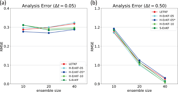
 is set to 1.2 as the optimal value. Analysis RMSE of LETKF in (c) is almost constant for localization radii from 6 to 19.
 is set to 5.0 in (a) and (c), and to infinity in (b) as the optimal values.


