Article
A Comparison between SAR Wind Speeds and Western North Pacific Tropical Cyclone Best Track Estimates
2024 Volume 102 Issue 5 Pages 575-593

Details
2024 Volume 102 Issue 5 Pages 575-593
Spaceborne synthetic aperture radar (SAR) for measuring high winds is expected to reduce uncertainties in tropical cyclone (TC) intensity and structure estimation, yet the consistency of SAR observed winds equivalent to a 1-min sustained wind speed with the conventionally estimated 10-min maximum wind speed (Vmax10) remains to be assessed. This study compares SAR wind observations with western North Pacific best track estimates from the Japan Meteorological Agency (JMA) and the Joint Typhoon Warning Center (JTWC). Because SAR wind observations have a bias dependent on SAR incidence angle, a first order corrective term is proposed and used to correct SAR-derived maximum wind (SAR Vmax) tentatively. After this correction, conversion of SAR Vmax into SAR Vmax10 with Dvorak conversion tables revealed a mean difference between SAR Vmax10 and JMA Vmax10 (ΔVmax10) of −0.1 m s−1 and a mean absolute difference of 4.8 m s−1. ΔVmax10 is found to be correlated with current intensities and with subsequent intensity changes from the SAR observation time. Also, comparison of the JMA best track 50-kt wind radius (R50) with SAR wind speeds suggests that R50 is systematically underestimated. Aside from the SAR wind limitations, possible reasons for the observed discrepancies between SAR wind observations and best track estimates include biases in the Dvorak analysis and conventional surface wind products. Further accumulation of SAR wind observations with appropriate bias correction in the future is expected to contribute to a comprehensive evaluation and improvement of conventional Vmax estimation methods, which could also be useful to verify TC intensity forecasts.
Real-time observations and forecasts of violent winds associated with tropical cyclones (TCs; see the Appendix for acronyms used in this paper) are essential for effective measures to be taken for disaster prevention. Aircraft reconnaissance in the North Atlantic has played an important role in monitoring high winds and TC structures and improving wind forecasts (e.g., Zawislak et al. 2022). Until recently, however, there have been no satellite instruments able to observe high winds with high spatial resolution under TC conditions (e.g., Knaff et al. 2021). In general, horizontal resolutions of conventional satellite wind products are too coarse, ∼ 10–50 km (e.g., Reul et al. 2017; Mayers and Ruf 2020), to observe TC fine structures. Also, because conventional scatterometers (e.g., the Advanced Scatterometer, ASCAT) saturate at high wind speeds above 18 m s−1 (Chou et al. 2013), the highest wind speeds are not observed. As a result, it has been difficult to verify the accuracy of best track estimates [maximum wind speed (Vmax), radius of maximum wind (RMW), etc.], and the resulting uncertainty is a serious issue for TC monitoring and forecasting in areas where there is no aircraft reconnaissance.
The advent of synthetic aperture radar (SAR) has led to a breakthrough in observing high winds with high spatial resolution in the inner core of TCs (e.g., Mouche et al. 2017, 2019). Conventional scatterometers equipped with a co-polarization microwave active sensor observe the roughness of the ocean surface by emitting, for example, vertically (resp. horizontally) polarized waves and receiving vertically (resp. horizontally) polarized waves after backscattering by ocean surface waves. However, the co-polarized signal begins to saturate or at least to decrease significantly its sensitivity to wind speed at high winds above 15 m s−1 (Donnelly et al. 1999). Most SAR systems can now emit in one polarization (vertical or horizontal) and receive in both polarizations (vertical and horizontal). The cross-polarized signal is more sensitive to volume scattering by breaking waves than the co-polarized signal (Zhang et al. 2017). Because the occurrence of breaking waves increases with wind speed, the volume scattering, i.e., the cross-polarized signal, observed as a normalized radar cross section (NRCS), also increases with wind speed (Phillips 1988; Hwang et al. 2010). Although open questions remain regarding the relative importance of surface and volume scattering, these two scatterings are the basic principles behind high wind speed estimates made by SAR. SAR wind speeds are retrieved by using geophysical model functions (GMFs) that relate the strength of the cross-polarization NRCS to 1-min sustained ocean winds observed by the Stepped Frequency Microwave Radiometer (SFMR, Uhlhorn and Black 2003; Uhlhorn et al. 2007). Mouche et al. (2019) and Combot et al. (2020) showed by using independent observations that SAR wind speeds with a horizontal resolution of 3 km are in good agreement with 1-min sustained ocean winds from the SFMR (Uhlhorn and Black 2003; Uhlhorn et al. 2007) with root mean squared error (RMSE) < 5 m s−1.
Radarsat-2 (RS2), Radarsat-C1/C2/C3 (Radarsat Constellation Mission, RCM), Sentinel-1A (S1A), and Sentinel-1B (S1B) satellites equipped with C-band SARs with a wide swath mode can observe TCs twice a day in a sun-synchronous sub-recurrent orbit with a local time of ∼ 06:00 on the descending node and ∼ 18:00 on the ascending node [e.g., Radarsat-2, European Space Agency (ESA) 2012]. While these C-band SARs have the same capabilities, the Sentinel (S1A and S1B), RS2, and RCM instruments are slightly different. In addition, Isoguchi et al. (2021) are currently working to develop a new SAR wind product that uses the Phased Array L-band Synthetic Aperture Radar-2 (PALSAR-2) aboard the Advanced Land Observing Satellite-2 (ALOS-2), whose local solar time is ∼ 12:00 on the descending node and ∼ 00:00 on the ascending node [Japan Aerospace Exploration Agency (JAXA) 2024]. Because SAR observations can have a 12-hourly frequency (or, 6-hourly in the future if ALOS-2/PALSAR-2 joins the TC observation community), SAR wind speeds have many potential uses and applications (e.g., Ricciardulli et al. 2023), including for intensity estimation (Howell et al. 2022), wind radii monitoring (e.g., Center for Satellite Applications and Research 2024), and data assimilation by operational numerical model systems for TC prediction (Ikuta and Shimada 2024). Even lower frequency observations can be useful for constructing an ocean truth dataset for estimation of a TC wind field through application of a statistical regression method to relate them to other data (e.g., Tsukada and Horinouchi 2023; Avenas et al. 2023). To realize such goals in the future, comparisons between conventional best track estimates and SAR wind speeds are necessary. Such comparisons can lead to more effective use of SAR wind speeds and improvements to TC intensity and wind radii estimates.
Combot et al. (2020) compared SAR Vmax with the Joint Typhoon Warning Center (JTWC) and National Hurricane Center (NHC) best track estimates of 1-min maximum wind (Vmax, Joint Typhoon Warning Center 2024; National Hurricane Center 2024) and showed that, although SAR Vmax is generally consistent with best track 1-min Vmax, the root mean squared difference (RMSD) is large in areas where no SFMR observations are available (e.g., in the western North Pacific). It is still unclear, however, how consistent 1-min SAR wind speeds are with best track 10-min Vmax (Vmax10) values estimated by the Japan Meteorological Agency (JMA, Japan Meteorological Agency 2024). JMA estimates Vmax10 primarily based on the Dvorak technique and its own conversion table (i.e., Koba table, Koba et al. 1991). Moreover, previous JMA Vmax10 had been derived mainly from the central pressure using Takahashi’s equation (Takahashi 1952) until the 1980s (Aizawa et al. 2024). The Koba table, used today, was created based on those JMA Vmax10 values. Takahashi’s equation was empirically made using maximum 20-min average wind speeds observed in islands and coastal areas for TCs (Takahashi 1940). Because of these historical reasons, it is well known that JMA Vmax10 values do not correspond linearly with 1-min Vmax values of JTWC by multiplying a factor of 0.88 or 0.93 (e.g., Mei and Xie 2016; Harper et al. 2010) as is done by several Regional Specialized Meteorological Centres (RSMCs). Therefore, it is important to investigate how to convert 1-min SAR Vmax values into Vmax10 values that match the conventional JMA values.
The purpose of this study is to investigate the consistency and differences between SAR wind speeds and conventional best track estimates for TCs in the western North Pacific, where no operational TC reconnaissance flights in the inner core are conducted except near Hong Kong (Hon and Chan 2022). Variables in the investigation include Vmax10, the radius of the 30-kt wind speed (R30), and the radius of the 50-kt wind speed (R50) from JMA best track data. Vmax and RMW from the JTWC best track data are also examined for comparison. Through these examinations, we highlight the need to continue improving the quality of SAR wind products and to comprehensively evaluate conventional estimation techniques for future work. Section 2 describes the datasets used and the methodology in this study. Section 3 presents the results of the examination. Section 4 discusses challenges and potential uses and applications of SAR wind observations. Section 5 provides conclusions of this study.
We used C-band SAR wind products from the CyclObs database (Vinour et al. 2023), provided by an IFREMER (French Research Institute for Exploitation of the Sea) team, with a horizontal resolution of 3 km. Table 1 provides basic information on C-band SAR acquisition modes whose products were used in this study. Because 3-km SAR wind speeds are in good agreement with 1-min sustained ocean winds from the SFMR (Mouche et al. 2019; Combot et al. 2020), the 3-km SAR wind speeds are considered to be equivalent to the 1-min sustained wind speed (e.g., Ricciardulli et al. 2023). In addition, the effect of rain attenuation on wind speed must be considered. In areas of strong rainfall, backscattered radar power can be decreased, resulting in decreases in retrieved wind speeds (by 5–10 m s−1, Mouche et al. 2019). Also, it is known that C-band SAR suffers from the effect of hydrometeors in the melting layer on wind speed (Mouche et al. 2019; Alpers et al. 2021), which can lead to overestimated wind speeds primarily observed along the outer rainbands. Furthermore, SAR wind speeds have an incidence-angle-dependent bias (e.g., Ikuta and Shimada 2024). We examine this incidence-angle-dependent bias in Section 3.

For this study, we collected 191 SAR wind observation files from 2012 to 2021 for TCs in the western North Pacific. However, after exclusion of cases with large data gaps within 100 km of the TC center and on the right side of the storm track, and landfalling cases, Vmax could be computed for 117 cases (61 %). Although this study relies on the results of Combot et al. (2020), who confirmed a good agreement between SFMR and SAR wind speeds, it should be noted that the maximum retrieved value of CyclObs SAR wind speeds is 80.0 m s−1. Given that SFMR observed a surface wind speed of more than 90 m s−1 during Hurricane Patricia (2015) (Kimberlain et al. 2016) and JTWC Vmax can reach 85 m s−1 (i.e., the highest value in the Dvorak current intensity table), it is possible that the CyclObs SAR wind speeds are underestimated in the case of such an extremely intense storm.
Because the obtained SAR wind speeds are swath data with a horizontal resolution of 3 km, they are transformed into polar coordinate data by using the center position obtained by the method described in Section 2.2 and Cressman interpolation. The polar coordinates are 2 km in the radial direction and 0.7° in azimuth (i.e., 512 grid points in azimuth). Although these resolutions are arbitrary, they are determined to properly obtain wind structure parameters even with large TC sizes. Then, a simple quality control (QC) procedure is performed, in which outliers exceeding three times the standard deviation of winds (i.e., 3-sigma QC) at each radius in the polar coordinate system are removed. However, it is not possible to remove all outliers using this method.
Other data used in this study include JMA and JTWC best track data, JMA Dvorak analysis data, and sea-surface wind (ASWind) data (Nonaka et al. 2019) derived from infrared (10.4 µm) atmospheric motion vectors (AMVs, Shimoji 2017) at heights below 700 hPa from Himawari-8 target observations (Bessho et al. 2016). The spatial resolution of ASWind data is 10 km. ASWinds are calibrated against ASCAT winds by multiplying the low-level infrared AMVs by a reduction factor (0.76). We use ASWind data that have passed a QC process (Nonaka et al. 2019) from the start of Himawari 8 operations (July 2015) to 2021. The best track estimates (Vmax, R30, R50, center positions, and RMW) used are linearly interpolated to the SAR observation time. Hereafter, the 6-hourly synoptic time closest to the SAR observation time is set to t = 0 h.
2.2 Center finding processCenter finding of a TC is conducted by using an interpolated best track center as a first guess position. In this finding process, the center is defined as the point where the azimuthal-mean SAR wind speed is maximized, a similar definition to what TC observational studies have done (e.g., Marks et al. 1992; Lee and Marks 2000; Rogers et al. 2013). Considering the effect of the environmental wind and the effect of a false SAR wind maximum seen near the center (Li et al. 2013), we do not regard the point with the minimum SAR wind in the eye region as the TC center. More specifically, the center finding process is shown in Fig. 1 and as follows:
 ) centered on the center candidate to the center’s wind speed (SARwind) and excluding candidates with a ratio less than 1.5 or the 40th percentile of all ratios, whichever is more restrictive. In this study,
  is computed if wind data are available for more than half of the polar grids at a given radius.
 |
where r and λ are the radial and tangential directions, respectively; the overbar denotes the azimuthalmean; and the prime denotes the deviation from the azimuthal-mean. The symmetry is averaged within a radius of 100 km. Next, normalize  obtained in step 2 by the highest value among all
  values. Then, calculate the possible center index (PCI) of the symmetry multiplied by the
  for each center position candidate. Find the center position that has the highest PCI value.
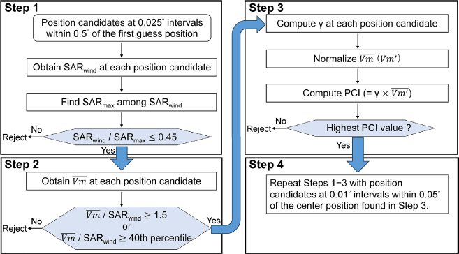
Schematic flow chart of the center finding process. See text for more details.
Although a reasonable center position can be objectively determined by the above procedure, it was not possible in two cases because of observational noise. Therefore, in those two cases, the center point was determined subjectively.
Here, we validate and compare SAR wind speeds. First, we briefly validate SAR with ASWinds. Second, we compare the seven nearly coincident SAR wind speed estimate cases to assess intra-SAR differences. Finally, we present the results of our comparison between SAR wind speeds and best track estimates.
3.1 Comparison with ASWindsASWinds are used for the estimation of R30 by JMA (Nonaka et al. 2019). ASWinds available within 1 km from SAR wind grid points and within 10 min of SAR observations are compared with SAR wind speeds in a two-dimensional histogram (Fig. 2). SAR wind speeds below 20 m s−1 are consistent with ASWinds with a standard deviation of less than 3 m s−1. However, SAR wind speeds greater than 20 m s−1 are much higher than ASWinds. This result is not surprising because of three reasons: (1) ASCAT winds tend to have negative biases caused by saturation at high wind speeds (e.g., Chou et al. 2013); (2) ASWinds are calibrated against ASCAT winds; and (3) the spatial resolution of ASWinds (10 km) is lower than that of SAR wind speeds (3 km). A more sophisticated technique to derive AMVs with a finer spatial resolution in a TC environment, such as one developed by Horinouchi et al. (2023), would be needed to partially resolve the negative bias issue.

Two-dimensional histogram of SAR wind speeds (m s−1) versus ASWinds (m s−1). The mean difference is 0.76, and the standard deviation (SD) is 2.66 m s−1. Only high-quality ASWinds with quality indicator (QI) (Holmlund 1998) values greater than 0.6 are used here. N is the total number of collocations, and Mean (X–Y) is the mean difference between SAR wind speeds and ASWinds.
Next, we intercompare SAR wind speeds observed nearly simultaneously (within 10 min) by two C-band SARs (RS2 and S1A or S1B). There are seven matchups that can be used for this purpose. Here, two SAR wind speeds are compared between the closest swath grid points. Figure 3 shows two-dimensional histograms of the match-ups. Overall, the mean absolute difference (MAD) is less than 2.5 m s−1, and at wind speeds below 20 m s−1, the wind samples are concentrated along the 1-to-1 line. For wind speeds greater than 20 m s−1, however, there are systematic differences between RS2 SAR wind speeds and Sentinel-1 (S1) SAR wind speeds:

Two-dimensional histograms of two C-band SAR wind speeds (m s−1). Radarsat-2 (R2) SAR wind speeds are plotted on the x-axis, and Sentinel-1A (S1A) or Sentinel-1B (S1B) SAR wind speeds are plotted on the y-axis. MAD is the mean absolute difference, and SD is the standard deviation. The mean incidence angles of RS2 SAR wind speeds and Sentinel-1 SAR wind speeds, in parentheses, are computed from match-ups with RS2 SAR wind speeds greater than 20.0 m s−1. Observation times are indicated in the axis labels.
In light of the angle-of-incidence-dependent bias, which will also be discussed in Section 3.3, these results seem reasonable if we consider that (i) there is a positive bias in the 20°–30° range and a negative bias in the 40–50° range and (ii) the magnitude of the bias differs between RS2 and S1. This certainly results from the accuracy of the GMFs with respect to the incidence angle and the instrument, and the quality of the signal within the swath in the range direction (incidence angle and elevation antenna gain pattern). To rectify this shortcoming, revisiting the GMFs using a larger sample of SAR collocations with reference wind measurements such as SFMR is certainly required. In addition, recent studies have revealed opportunities for improving the calibration of the SAR signal (Schmidt et al. 2023) and the noise correction (Korosov et al. 2022).
3.3 Maximum wind a. Relationship between best track Vmax and SAR VmaxWhen comparing best track Vmax with SAR wind speeds, it should be noted that the best track Vmax has a coarse time resolution (i.e., 6-hourly) and does not represent localized wind speed maxima (e.g., Franklin 2013). In contrast, SAR wind speeds are instantaneous and can reflect transient wind speed enhancements, but they also have outliers due to noise. In this study, we define SAR maximum wind speed (SAR Vmax) as the 99th percentile of SAR wind speeds at grid points within 200 km from the center in the polar coordinate system. The 99th percentile is determined as in Combot et al. (2020), although the grid point range is different. In a preliminary analysis, we found that outliers due to noise are almost always located above the 99th percentile. Because transient wind speed maxima should not be regarded as Vmax, the 99th percentile is a reasonable cutoff even if no outlier wind speeds are included in an observation. In this study, SAR Vmax is regarded as valid if SAR wind observations are available for more than half of the polar grids within 100 km from the center. Eight cases, however, are excluded where SAR wind observations are missing at the RMW on the right side of the storm track.
We first show how the difference between best track Vmax and SAR Vmax changes when different thresholds are used (Table 2). SAR Vmax values from the 99th percentile or above are much greater than JMA Vmax10 values. Because SAR wind speeds with a horizontal resolution of 3 km are considered to be greater than 10-min sustained wind speeds (e.g., Ricciardulli et al. 2023), it is expected for SAR Vmax to have a positive bias relative to JMA Vmax10. In contrast, SAR Vmax values from the 99th percentile or below are much smaller than JTWC best track Vmax. The fact that the maximum available SAR wind speed is 80.0 m s−1 may affect the JTWC bias, whereas the maximum JTWC best track Vmax is 87 m s−1 (170 kt, 1 kt = 0.5144 m s−1).

Figure 4 shows scatter plots of SAR Vmax versus JMA best track Vmax10 and versus JTWC Vmax. JMA Vmax10 values are much smaller than SAR Vmax values (MAD = 7.4 m s−1, Table 2), especially in the case of strong TCs. Even if we convert SAR Vmax values into Vmax10 values by a factor of 0.93, which is recommended by the World Meteorological Organization (WMO, Harper et al. 2010), the converted Vmax10 values are much higher than JMA Vmax10 values (MAD = 6.4 m s−1). If we depict the conversion relationship between Vmax10 and Vmax derived from the Dvorak conversion tables of Dvorak (1984) for Vmax and Koba et al. (1991) for Vmax10, we find that the data points are concentrated on the conversion line (Fig. 4a), in particular, in the case of strong TCs. Hence if we convert SAR Vmax values to 10-min values (hereafter, SAR Vmax10) using this conversion relationship, the differences between JMA Vmax10 and SAR Vmax10 (hereafter ΔVmax10, ΔVmax10 ≡ JMA Vmax10 – SAR Vmax10) become small; the mean ΔVmax10 is 0.4 m s−1, and its MAD is 5.5 m s−1. For JTWC Vmax, there is a rough 1-to-1 relationship between JTWC Vmax and SAR Vmax (Fig. 4b); the mean difference between JTWC Vmax and SAR Vmax (hereafter ΔVmax, ΔVmax ≡ JTWC Vmax – SAR Vmax) is −3.4 m s−1, and its MAD is 7.9 m s−1 (Table 2). Considering the difference in the range of Vmax values between JWTC and JMA, the level of the MADs for JTWC and JMA can be interpreted as nearly identical. JMA Vmax varies from 35 kt to 125 kt, while JTWC Vmax varies from 35 kt to 170 kt. Thus, the MAD of JTWC Vmax should be 1.5 times [i.e., (170-35)/(125-35)] larger than that of JMA Vmax10, which is almost the same as the actual 1.4 times (i.e., 7.9/5.5).

Scatter plots of SAR Vmax (m s−1) versus best track Vmax (m s−1) for (a) JMA and (b) JTWC. The black line indicates the 1-1 line. In (a), the orange line indicates the conversion line between the 10-min and 1-min sustained Vmax values by a factor of 0.93 (Harper et al. 2010). Also, the red circles are intensity points that relate the 1-min sustained Vmax Dvorak (1984) to the 10-min sustained Vmax (Koba et al. 1991) through Dvorak conversion tables, and the red line connecting them is the conversion line between the 10-min and 1-min sustained Vmax values.
Next, we further investigate the characteristics of ΔVmax10 for JMA and ΔVmax for JTWC. One possible cause of the variabilities of ΔVmax10 and ΔVmax is a bias that is dependent on SAR incidence angle, as described in Section 3.2. A scatter plot of the incidence angle at the TC center versus SAR Vmax (Fig. 5a) suggests that SAR Vmax values are dependent on the incidence angle. Thus, it seems that SAR Vmax derived from the current product is not suitable for quantitative use without any correction. However, in the absence of any true reference data (e.g., SFMR winds), it is not possible to estimate how much SAR Vmax is biased relative to a given incidence angle. Figures 5b and 5c show scatter plots of the incidence angle versus ΔVmax10 for JMA and versus ΔVmax for JTWC, respectively. If we assume that the incidence-angle-dependent bias of SAR Vmax10 and SAR Vmax is deduced from the deviation from the best track Vmax10 and Vmax, then SAR Vmax10 and SAR Vmax values associated with low incidence angles may have a positive bias and SAR Vmax10 and SAR Vmax values associated with high incidence angles may have a negative bias. This deduction is consistent with the results of the intercomparison between SAR wind products in Section 3.2.

Scatter plots of (a) incidence angle (°) versus SAR Vmax (m s−1) from (blue) RS2 and (S1, orange) S1A and S1B, (b) incidence angle (°) versus ΔVmax10 (JMA best track Vmax10 – SAR Vmax10, m s−1), and (c) incidence angle (°) versus ΔVmax (JTWC best track Vmax – SAR Vmax, m s−1). In (b), the linear lines indicate the linear relationships between ΔVmax10 and the incidence angles for (blue) RS2 SAR and (orange) S1 SAR expressed by Eq. (2). In (c), the linear lines indicate the linear relationships between ΔVmax and the incidence angles for (blue) RS2 SAR and (orange) S1 SAR expressed by Eq. (3).
Using the relationships between ΔVmax10 and ΔVmax and the SAR incidence angles for RS2 and Sentinel-1A and -1B (S1) shown in Figs. 5b and 5c, we can tentatively correct SAR Vmax10 and SAR Vmax, respectively, using the following linear relationships:
 |
 |
where the prime indicates the corrected value, and θ indicates the incidence angle in degrees. Although this bias correction method may be quantitatively rough, it eliminates the incidence-angle-dependent bias for the CyclObs SAR wind speeds. Figure 6a shows a scatter plot of SAR Vmax10′ versus JMA Vmax10. The correction makes ΔVmax10′ small; the mean absolute ΔVmax10′ is 4.8 m s−1. As for JTWC, the mean absolute ΔVmax′ is 6.7 m s−1 (Fig. 6b). Note that some SAR Vmax10′ and SAR Vmax′ with relatively poor coverage of SAR wind observations at the RMW might be underestimated, although cases with large data gaps at the RMW on the right side of the storm track are excluded. Hereafter the corrected SAR observations (i.e., ΔVmax10′, SAR Vmax10′, Δvmax′, and SAR Vmax′) are used. For reference, we confirm that the conclusions of this study are not changed even if uncorrected data are used.

Scatter plots of (a) SAR Vmax10′ (m s−1) versus JMA best track Vmax10 (m s−1) and (b) SAR Vmax′ (m s−1) versus JTWC best track Vmax (m s−1). The black line indicates the 1-1 line. MAD is the mean absolute difference. Colors indicate the coverage (%) of SAR wind observations at the RMW.
Another possible cause of the variabilities of ΔVmax10′ and ΔVmax′ is associated with best track Vmax. Figure 7 shows that ΔVmax10′ and ΔVmax′ are correlated with best track Vmax10 and Vmax, respectively, at the time of the SAR observations (t = 0 h); best track Vmax values of weak TCs tend to be lower than SAR Vmax and those of intense TCs tend to be higher than SAR Vmax. Table 3 shows that their correlation coefficients (r) are 0.77 for JMA and 0.73 for JTWC, respectively. It is unclear, however, whether these correlations are due to a bias of SAR Vmax or to a bias of best track Vmax.

Scatter plots of (a) JMA Vmax10 (m s−1) versus bias-corrected ΔVmax10′ (JMA best track Vmax10 – SAR Vmax10′, m s−1) and (b) JTWC Vmax (m s−1) versus bias-corrected ΔVmax′ (JTWC best track Vmax – SAR Vmax′, m s−1). Colors in (a) indicate JMA Vmax10 changes in the next 24 h from t = 0 h (i.e., the 6-hourly synoptic time closest to the SAR observation time). Colors in (b) indicate JTWC Vmax changes in the next 36 h from the time of SAR observations. The “x” mark with a gray circle plotted in some of the circles indicates TCs that made landfall within 24 h in (a) and 36 h in (b). Note that TCs that disappeared or became extratropical cyclones before the end of the period of intensity changes are not included in these plots because of the lack of best track Vmax data.

Table 3 also shows correlations between ΔVmax10′ and Vmax10 changes for JMA and between ΔVmax′ and Vmax changes for JTWC. Although it is natural for weak TCs to intensify and for intense TCs to weaken, it is interesting that there is a clear relationship within the range from 30 m s−1 to 50 m s−1 for JMA (Fig. 7a); weakening (i.e., negative Vmax changes) and steady-state (i.e., no Vmax change) TCs tend to have a positive ΔVmax10′ and intensifying (i.e., positive Vmax changes) TCs tend to have a negative ΔVmax10′. Note that weakening TCs with a negative ΔVmax10′ include TCs landfalling within 24 h after the SAR observations (Fig. 7a). Also, among the eight TCs that experienced extratropical transition (ET) within 24 h after the SAR observations, seven were weakening TCs with negative ΔVmax10′ (not included in Fig. 7a because of the lack of best track Vmax10 estimates since ET). For JTWC, a similar correlation is seen but it is weaker than that of JMA (Fig. 7b, Table 3). The stronger correlation of JMA Vmax10 changes with ΔVmax10′ may suggest that JMA best track Vmax10 has a time lag relative to SAR Vmax10.
Best track Vmax values are primarily estimated by the Dvorak technique (Dvorak 1984) with some modifications based on all available observations, including conventional satellite-derived winds such as ASCAT and winds observed on islands. Knaff et al. (2010) evaluated Dvorak intensity estimates with reference to aircraft observation-based best track Vmax values and found that systematic biases in Dvorak intensity were a function of best track Vmax, best track Vmax change trend, translation speed, latitude, and TC size. We also find that R30 is correlated (r = 0.37) with ΔVmax10′, likely because R30 is correlated with intensity (r = 0.37). There is no correlation of ΔVmax10 with translation speed or latitude (r = −0.09, −0.01, respectively). The characteristics of JMA Vmax10 are consistent with the results of Knaff et al. (2010), except those for latitude and translation speed, and thus may be attributed to the use of the Dvorak technique.
c. Characteristics of ΔVmax10′ stratified by intensity changesHere, we further examine characteristics of ΔVmax10′ stratified by intensifying, steady-state, weakening, and extratropical transitioning TCs in relation to the Dvorak analysis. Intensifying, steady-state, and weakening cases are defined as cases with a positive JMA Vmax10 change, no 24-h JMA Vmax10 change, and a negative JMA Vmax10 change from t = 0 h to t = 24 h, respectively. Among 117 cases in the SAR dataset used, there are 102 cases with a Vmax10 change from t = 0 h to t = 24 h in JMA best track data; 34 intensifying cases, 21 steady-state cases, and 47 weakening cases (Fig. 7a). The remaining 15 cases include eight ET cases, five TCs that became a tropical depression or dissipated, and two storms whose Vmax10 values are undefined at t = 0 h due to the lack of best track Vmax10 estimates near the time of ET.
Among 34 intensifying cases, more than half (21 cases, 62 %) have negative ΔVmax10′ less than −1 m s−1, whereas only 15 % (five cases) have positive ΔVmax10′ more than 1 m s−1 (Fig. 7a). The mean SAR Vmax10′ of these 21 cases is 35.2 m s−1, whereas the mean JMA Vmax10 is 29.3 m s−1. Of the 21 cases, more than half (57 %) have small RMWs of less than 25 km, and 76 % have RMWs less than the overall mean RMW of 41.4 km (Fig. 8a). Also, the vast majority (90 %) are TCs before reaching the Dvorak eye pattern, such as organized cumulonimbus (Cb) clusters, central dense overcast (CDO), or a curved band-type pattern (Fig. 8b). Velden et al. (2006) pointed out that Dvorak intensities of TCs with such cloud patterns tend to be underestimated, and Knaff et al. (2010) found that rapidly intensifying TCs tend to be underestimated by Dvorak analysis. Although SAR Vmax10′ may still show a bias, the result here is consistent with those of previous studies. Figure 8c shows Typhoon Jongdari (2018) as an example. SAR Vmax10′, though it has quantitative uncertainty, is much greater than JMA Vmax10 during the intensification stage of Jongdari (2018). Also, Jongdari (2018) was characterized by a small RMW (14–18 km) and a compact structure (Figs. 8d, e).

Frequency histograms of (a) SAR-derived RMWs (km) and (b) Dvorak cloud patterns of the 20 intensifying TCs with negative ΔVmax10′. (c) Temporal evolution of the JMA best track Vmax10 (black line, m s−1) and the SAR Vmax10′ (red circles, m s−1) for Typhoon Jongdari (2018). (d, e) SAR wind distributions for Typhoon Jongdari (2018) at (d) 2055 UTC 24 July and (e) 2045 UTC 25 July. The black circle in (d) and the outer black circle in (e) is JMA R30; in (e), the inner red circle is the JMA R50. Cb and CDO in (b) are cumulonimbus and central dense overcast, respectively.
Among 21 steady-state cases, 15 (71 %) cases have JMA Vmax10 greater than SAR Vmax10′ (Fig. 7a). Of these 15 cases, 14 have cloud patterns associated with TC eyes and Vmax10 values above 40 m s−1 in all 15 cases (not shown). In short, mature TCs tend to exhibit these features.
Among 47 weakening cases, the majority (33 cases, 70 %) have positive ΔVmax10′ greater than 1 m s−1, whereas only 21 % (10 cases) have negative ΔVmax10′ less than −1 m s−1 (Fig. 7a). The mean SAR Vmax10′ of these 33 cases is 40.7 m s−1, whereas the mean JMA Vmax10 is 46.2 m s−1. Most of the 33 cases are TCs during and just after the mature stage, and 67 % of the 33 cases are associated with a TC eye (not shown). Typhoon Halong (2019) is a typical example of a weakening TC (Figs. 9a, b).

(a) Temporal evolution of JMA best track Vmax10 (black line, m s−1) and SAR Vmax10′ (red circles, m s−1) of Typhoon Halong (2019), and (b) the SAR wind distribution for the typhoon at 1957 UTC 5 November. The inner red circle indicates JMA R50, and the outer black circle indicates JMA R30. (c) Box-and-whisker plots of the ΔVmax10′ (m s−1) samples of 53 weakening cases stratified by the difference between CI number and T number (CI number minus T number) from the Dvorak analysis. The “×” marks indicate the mean, and the numbers of positive and negative ΔVmax10 samples are shown in parentheses from left to right.
For the majority of weakening cases, the positive ΔVmax10′ might be associated with the Dvorak time lag rule, in which the current intensity (CI number) remains higher than that estimated from the cloud pattern (T number) during the weakening stage (Lushine 1977). In fact, 61 % of the 33 cases with positive ΔVmax10 greater than 1 m s−1 have a CI number higher than their T number (Fig. 9c); the mean CI number is 5.7, whereas the mean T number is 5.3. According to the table provided by Koba et al. (1991), a difference in the CI number of 0.5 is equivalent to ∼ 3.6 m s−1. JMA has a 12-h time lag rule, following Lushine (1977). However, it has been pointed out that the 12-h lag is too long (Brown and Franklin 2004). Knaff et al. (2010) mentioned the possibility that the final T-number constraints of the Dvorak analysis give a positive intensity bias to weakening TCs. Although it is possible that the positive ΔVmax10 is simply caused by a negative bias of SAR Vmax10 converted from SAR Vmax using Dvorak tables for high winds, the finding here is consistent with previous studies.
Although the number of cases is small, all six TCs that completed ET without having made landfall within 24 h after SAR observations have SAR Vmax10 greater than best track Vmax10 (Fig. 10). This result suggests that the best track Vmax values of extratropical transitioning TCs may be underestimated. This underestimation may be because the Dvorak technique does not capture Vmax at the time of the ET. We also examine the relationship between the direction of vertical wind shear, the direction of translation, and the position of SAR Vmax (Fig. 11) for these six TCs. Generally, the TC wind maximum is located on the front right side with respect to the translation direction (Shapiro 1983; Kepert and Wang 2001). However, some extratropical transitioning TCs are characterized by a wind speed maximum located on the left side with respect to the translation direction (Figs. 11c, e, f), which is also the left side with respect to the vertical shear direction. This feature is consistent with the findings of Ueno and Kunii (2009), who showed that some TCs have a wind maximum on the left with respect to the TC translation direction only when the vertical shear direction is close to the TC translation direction. Furthermore, the extratropical transitioning TCs tend to have a wavenumber-2 asymmetric wind structure (Figs. 11d–f). The wavenumber-2 wind structure is one of the typical wind distribution patterns of TCs that make landfall on the main islands of Japan (Fujibe and Kitabatake 2007; Kitabatake and Fujibe 2009; Loridan et al. 2014).

JMA best track Vmax10 and SAR Vmax10′ of extratropical transitioning TCs.

SAR wind distributions of the six TCs that completed ET without having made landfall within 24 h after SAR observations. The direction of vertical wind shear (blue arrows) and the translation direction (black arrows) are shown together with their magnitudes (blue and black numerals). The vertical wind shear is defined as deep-layer (850–200 hPa) shear, which is the mean shear within 500 km from the TC center using the Japanese 55-year Reanalysis (JRA-55) data (Kobayashi et al. 2015). The translation speed is calculated by a 12-h centered difference in the JMA best-track position. The red circle indicates JMA R50, and the black circle indicates JMA R30.
We compare the RMWs between SAR and JTWC. Note that RMW values in the JTWC best track are not reanalyzed following the season (Joint Typhoon Warning Center 2024) and are the consequence of the need to provide an RMW for TC vitals and input to numerical weather prediction. In this study, the RMW is defined as the radius of maximum azimuthal-mean SAR wind, the same as Tsukada and Horinouchi (2023), in consideration of the incidence-angle-dependent bias and the rain attenuation bias in SAR wind speeds. This definition is slightly different from that of JTWC, according to which the RMW is the radius of local Vmax. For intense TCs, however, the difference between these two definitions is not expected to result in significantly different RMWs because both RMWs should be located near the eyewall. Figure 12a shows that the MAD between JTWC and SAR RMWs is 22.1 km with a correlation coefficient of 0.34. This result is consistent with Fig. 12b of Combot et al. (2020).

(a) Scatter plot of JTWC RMWs (km) versus SAR RMWs (km) below 140 km. (b) Scatter plot of JTWC Vmax (m s−1) versus SAR RMWs (km) and (colors) two-dimensional histogram of JTWC Vmax (m s−1) versus JTWC RMWs (km) during the period of 2011–2021. (c) As in (b), but for scatter plot of bias-corrected SAR Vmax (m s−1) versus SAR RMWs (km). In (a), the black circles are the same as those in area I in (b), and the red circles are the same as those in area II in (c). In (b, c), the black and red boxes correspond to areas I and II, respectively.
Figures 12b and 12c show scatter plots of SAR RMWs versus JTWC Vmax values and versus SAR Vmax values, respectively, and the frequency distribution of JTWC RMWs versus JTWC Vmax during the period of 2011–2021. Most of the observed cases in Fig. 12b are concentrated on the frequency distribution of JTWC best track estimates. However, two low frequency areas of the best track estimates have some observed cases. One is area I defined as the area of Vmax values with 15–30 m s−1 and RMWs with 0–30 km. Area I has 13 observed cases in Fig. 12b. These 13 cases are characterized by large differences in Vmax and RMWs between SAR observations and JTWC estimates. Twelve cases among the 13 cases have SAR Vmax′ much greater than JTWC Vmax; the mean SAR Vmax′ of the 12 cases is 33.1 m s−1, whereas the mean JTWC Vmax is 23.5 m s−1. As a result, there are only five cases in area I of Fig. 12c. All SAR RMWs of the 13 cases are much smaller than JTWC RMWs (Fig. 12a).
Another is area II defined as the area of Vmax values with 30–60 m s−1 and RMWs with 60–140 km. Area II has 20 observed cases in Fig. 12c. Of these 20 cases, 95 % have SAR RMWs much larger than JTWC RMWs (Fig. 12a), and 85 % are weakening TCs or TCs just after eyewall replacement cycles (not shown). JTWC best track estimates, however, rarely contain such large RMW cases with Vmax values with 30–60 m s−1. With the accumulation of SAR wind observations, the climatological relationship between Vmax and RMWs in the western North Pacific found in JTWC best track estimates may be completely updated in the future.
b. R30 and R50The swath range of SAR observations does not cover the entire R30 and R50 regions. Therefore, in this study, to investigate the consistency between JMA best track R30 and R50, and the SAR wind distribution, SAR wind speeds on the R30 and R50 circles are divided into wind speed bins. In JMA, R30 is defined as the radius within which a 10-min sustained wind speed greater than 30 kt (∼ 15 m s−1) exists or “potentially” exists, and R50 is defined similarly. Thus, SAR wind speeds on the R30 and R50 circles are expected to be lower than 15 m s−1 and 25 m s−1, respectively. Here, we use temporally interpolated R30 and R50 values. Also, we use SAR wind speeds transformed onto the polar coordinates so that the number of wind samples at each radius is the same regardless of the TC size.
Figure 13 shows SAR wind speeds observed on the R30 and R50 circles using 2.5 m s−1 and 5.0 m s−1 bins, respectively. The best track R30 is generally consistent with the SAR wind speeds; winds on the R30 circle are mostly (88 %) less than 15 m s−1. The cause of the underestimation in 12 % of the R30 samples would include the bias in SAR wind speeds and the effect of strong environmental wind speeds, such as monsoon flow, as well as the actual underestimation of R30. In contrast, on the R50 circle, 28 % of the samples have wind speeds of 25 m s−1 or higher. The best track R50 tends to be underestimated even if the difference between 1-min and 10-min sustained wind speeds is considered. We suspect that the underestimation of the best track R50 is caused by the use of ASWinds and scatterometer winds that have a low bias for winds greater than 20 m s−1 (e.g., Fig. 3).

Frequency histograms of SAR wind speeds on the JMA (a) R30 and (b) R50 circles.
Although SAR Vmax is equivalent to 1-min wind speed, it is consistent with JMA Vmax10 if we convert SAR Vmax into SAR Vmax10 with two Dvorak conversion tables used at JMA and JTWC. This finding is helpful to use the brand-new SAR wind observations in a way consistent with conventional JMA Vmax10. We should, however, be aware that this conversion method is a by-product for convenience when the Dvorak technique is the main tool for estimating TC intensity. According to Harper et al. (2010), the wind speed conversion factor from 1-min to 10-min values is recommended to be 0.93, which is independent of wind speed. This factor is derived from the relationship between mean wind and a gust factor. Therefore, the wind speed conversion should essentially be done that way. It is possible that SAR-based wind observations can be a main source for estimating TC intensity in the future instead of the Dvorak technique if the frequency of SAR observations greatly increases. Then, a time may come when a decision has to be made as to whether SAR Vmax should be converted into Vmax10 that is consistent with conventional JMA Vmax10 or whether SAR Vmax should be converted into Vmax10 by a factor of 0.93.
The comparison between JMA Vmax10 and SAR Vmax10′ in Section 3.3 suggests that weakening and steady-state TCs that have reached a certain level of intensity may tend to be overestimated in the Dvorak analysis. Also, the negative correlation between ΔVmax10′ and future intensity changes suggests that the JMA Vmax10 lags behind SAR Vmax10′ during the intensifying stage and at the start of weakening stage; that is, actual Vmax10 may increase earlier and start to decrease earlier than JMA Vmax10. After more SAR wind observations have been accumulated and the incidence-angle-dependent bias has been improved, whether these issues really exist in the Dvorak analysis and JMA Vmax10 should be comprehensively investigated.
Currently, it is not easy to estimate wind structure parameters such as the RMW and R50 in the western North Pacific, where aircraft observations are not available. With the advent of SAR wind observations as a truth dataset, it will be operationally possible to estimate wind structure parameters by a statistical approach using infrared satellite cloud patterns (e.g., Kossin et al. 2007; Knaff et al. 2015; Tsukada and Horinouchi 2023) or a set of easily available parameters including an outer wind radius, the Coriolis parameter, and Vmax (Chavas and Knaff 2022; Avenas et al. 2023). The development of such a method will help to further improve the best track estimates. We will perform this work in the future.
This study compared SAR wind speeds provided by CyclObs with best track 10-min Vmax and wind radii provided by JMA to examine the consistency between brand-new high wind products and conventional TC best track estimates. We also examined best track 1-min Vmax and RMWs provided by JTWC for comparison. The SAR-derived maximum wind (SAR Vmax) was defined as the 99th percentile value of SAR wind speeds at grids within 200 km from the TC center in order to exclude outliers and transient wind speed maxima. Furthermore, SAR Vmax, which is considered to be the 1-min sustained wind speed, was converted into 10-min Vmax (SAR Vmax10) by using Dvorak conversion tables for JTWC’s 1-min Vmax and JMA’s 10-min Vmax. Because SAR Vmax shows a bias that is dependent on SAR incidence angle, in this study, we tentatively corrected SAR Vmax (SAR Vmax′) and SAR Vmax10 (SAR Vmax10′) using a first order corrective term. After the correction, we found that SAR Vmax10′ is consistent with JMA Vmax10; the mean difference between them (ΔVmax10′) is −0.1 m s−1, and the mean absolute difference is 4.8 m s−1. The mean difference between SAR Vmax and JTWC Vmax (ΔVmax′) is −0.1 m s−1, and the mean absolute difference is 6.7 m s−1. We also found that ΔVmax10′ was a function of current intensity and intensity changes up to 24 h to 36 h in the future. Cases with negative ΔVmax10′ mostly include intensifying TCs or extratropical transitioning TCs. Most of the intensifying TCs are at the stage before the TC eye appears in infrared satellite imagery; this result may be related to the well-known negative bias of the Dvorak analysis. Also, it can be seen that it is not easy to estimate Vmax10 for extratropical transitioning TCs by conventional methods. In contrast, cases with positive ΔVmax10 mostly include steady-state or weakening TCs. One possible cause of the positive bias is the 12-h time lag rule of Dvorak intensity for steady-state and weakening TCs, according to which the current intensity remains higher than the intensity derived from cloud patterns. There are large differences in the RMWs between SAR observations and JTWC estimates. Some of the cases with large RMW differences are characterized by cases with SAR Vmax much greater than JTWC Vmax, cases with intense, but weakening TCs, and cases just after eyewall replacement cycles. These results reveal that JTWC’s RMW estimates are largely a function of intensity, that is a climatology, and are, at times, much different from the observed (also see Combot et al. 2020 and Avenas et al. 2024). This is not surprising due to the need to provide this information for the guidance suite, but users of the existing RMW should be aware of this shortcoming in the records. The comparison between JMA’s R30 and R50 and SAR wind speeds showed that best track R30 is generally consistent with SAR wind speeds, whereas best track R50 is underestimated relative to SAR wind speeds. This underestimation may be because, for winds above 18 m s−1, scatterometer (e.g., ASCAT) winds and AMV-derived winds (ASWinds) used to estimate R50 have a negative bias.
The time has come when a thorough review and revisitation of conventional methods such as the Dvorak technique are both necessary and possible with the emergence of the new SAR observation instrument. SAR wind observations still have some limitations. The derivation of a GMF to relate the ocean surface wind speed to the radar signal under extreme conditions, properly accounting for the incident angle effect, is an ongoing area of research. Future work, however, will allow the comprehensive evaluation of conventional methods through the accumulation of SAR wind observations for many TCs. These efforts will also contribute to the verification and improvement of TC intensity forecasts.
SAR wind products are provided by the CyclObs website (https://cyclobs.ifremer.fr). The best track data from JMA are available on their website (https://www.jma.go.jp/jma/jma-eng/jma-center/rsmc-hp-pub-eg/trackarchives.html). The best track data from JTWC are available on their website (https://www.metoc.navy.mil/jtwc/jtwc.html?western-pacific). ASWinds are obtained from the Himawari JDDS website (https://www.jma.go.jp/jma/jma-eng/satellite/jdds.html) although only National Meteorological and Hydrological Services can have access to the data. The JMA Dvorak analysis data are not publicly available due to restrictions.
U. Shimada and M. Hayashi are deeply grateful to their colleagues in JMA Headquarters who provided the Dvorak analysis data and ASWind data. The constructive suggestions from two reviewers are appreciated. The opinions in this paper are those of the authors and should not be regarded as official JMA views. This work was supported by MEXT KAKENHI Grant 21H01164 and 23K13172. A. Mouche acknowledges the support from ESA MAXSS and ESA MPC-S1 projects.