Abstract
A high-resolution sea surface temperature (SST) analysis called COBE-SST3 covers daily to centennial SST variations. The SSTs were constructed by performing analyses for low-frequency components, interannual variations, and daily changes with statistical methods using in-situ and satellite observations. The biases for each observation type were objectively estimated, and the result was a reconfirmation that the types are not properly categorized in the international database. By introducing a correction to the global mean nighttime marine air temperature observations which is used for the bias detection, moderate changes in global mean SSTs around World War II were obtained in COBE-SST3. SST and land surface air temperature (LSAT) fields were simultaneously analyzed on a monthly time scale for consistency between SST and LSAT. The LSAT observations acted as low-quality SST observations, and could produce SST variations to an eye-opening degree. This is the same as in the SST observations. The simultaneous analysis suggested that SST and LSAT observations were complementary and of satisfactory quality. Two types of daily SST analyses on a 0.25° grid were produced: one is a blend of multiple satellite and in-situ observations, and the other is a reconstruction with in-situ observations only. The two analyses were highly correlated with a counterpart provided by the National Oceanic and Atmospheric Administration of the USA. Uncertainties in low-frequency components, interannual variations, daily changes were separately estimated. These were used to construct daily perturbed SSTs, which are random, normally distributed, and spatiotemporally continuous.
1. Introduction
Sea surface temperatures (SSTs) and land surface air temperatures (LSATs) are the longest known variables based on instrumental measurements over the Earth. Many efforts have been made not only to maintain the measurements but also to unearth the buried data. These observations have been used to understand long-term past climate changes (Paltridge and Woodruff 1981; Jones et al. 1986; Barnett 1984).
Global warming signals in global mean temperatures or local SST changes of high interest are sometimes smaller than observational biases in the past SST record. Folland and Parker (1995) summarized the sources of SST observation biases. For example, uninsulated bucket observations suffer from cold biases due to exposure of the bucket to cold air for a long time on the ship deck, and conversely, engine room intake (ERI) SSTs include warm biases. Because many metadata on observation type are missing or not always correctly specified in the International Comprehensive Ocean-Atmosphere Data Set (ICOADS; Woodruff et al. 1987; Freeman et al. 2017), a serious problem remains: how to quantify the biases of individual reports. Based on the literature and indoor experiments, Folland and Parker (1995) proposed time-varying bias corrections. Unknown types since the mid-20th century are thought to be a mixture of insulated and uninsulated buckets and ERI. Kennedy et al. (2011) estimated the fractions of each based on the literature. The metadata of WMO Publication No. 47 are available and can complement ICOADS (Kent et al. 2007). However, the metadata are very limited before the 1960s. Several approaches to remove the biases have been proposed by Smith and Reynolds (2002), Kent et al. (2010), Hirahara et al. (2014), and Chan and Huybers (2019), but the uncertainties in low-frequency SSTs remain large before 1980, where recent high-precision observations such as drifting buoys and Argo floats are not available. The Hadley Center nighttime air temperature version 2 (HadNMAT2; Kent et al. 2013) has widely been used to estimate the SST biases in the Extended Reconstruction SST version 4 (ERSST4; Huang et al. 2015) and the Hadley Center SST version 4 (HadSST4; Kennedy et al. 2022), which compared SSTs and Nighttime Marine Air Temperatures (NMATs) for spatiotemporal consistency between the two variables. Despite years of effort, SSTs around World War II suffer from large uncertainties due to the data gaps and poor metadata (Rayner et al. 2006).
The observations on land are made at the same location over a long period. This makes it easier to evaluate biases and detect the erroneous records than the maritime observations made at the different locations. In contrast, the land surface is not thermodynamically stable due to its small specific heat capacity. In addition, the topography is complex. Because of long-term LSAT studies, the literature on the observations is extensive. For example, data gaps due to station relocations and environmental changes in the measurements have been homogeneously adjusted in neighboring areas (Osborn and Jones 2014), and various sources of LSAT uncertainties including urbanization have been investigated (Menne et al. 2018). These activities have led to the archiving of international databases: Global Historical Climatology Network version 4 (GHCN4; Menne et al. 2018) and the International Surface Temperature Initiative (ISTI) Global Land Surface Temperature Databank (Thorne et al. 2011; Noone et al. 2021).
In general, historical analyses are defined generally on monthly 1–2° grids without the use of satellite observations. Recently, the Hadley Center have provided a reconstructed daily 0.25° analysis known as HadISST2 that was used for the Coupled Model Intercomparison Phase 6 (CMIP6). The NOAA/USA Daily OISST version 2 (Reynolds et al. 2007) was merged to form the high resolution HadISST (Haarsma et al. 2016). For such high-resolution SSTs, satellite observations are needed in order to resolve mesoscale ocean eddy activities. With multiple satellite SSTs, operational centers produce hourly-daily global 0.01–0.25° SST analyses (Yang et al. 2021). In many satellite analyses, both the satellite and in-situ observations are blended in them. These high-resolution analyses increase the variances and the gradients, compared with low-resolution SST analyses.
The uncertainty information on SST could be useful in various climate studies. The SST analysis includes unavoidable errors due to the data sparseness or observational errors, and therefore, a single analysis may sometimes overestimate or underestimate climatic signals in local or basin-scale SST variations. Perturbed SSTs proportional to the uncertainties varying in space and time are frequently used to obtain probabilistic responses of atmospheric models to observed SST. The climate simulation result called database for policy decision making for future climate change (d4PDF) was produced (Mizuta et al. 2017), and it has been widely used for climate and impact assessment studies (Ishii and Mori 2020). A historical atmospheric reanalysis, Over-centennial Atmospheric Data Assimilation (OCADA), used the same perturbations that expand the model spreads of an ensemble Kalman filter (Ishii et al. 2024). In d4PDF and OCADA, the perturbations were constructed from COBE-SST2 (Hirahara et al. 2014, hereafter HIF14).
The subsequent sections provide a brief introduction of COBE-SST3 in Section 2, descriptions of observations and methodologies used in this study in Sections 3 and 4, and demonstrations of the new SST and LSAT analyses. Finally, concluding remarks are given in Section 6.
2. Overview of new COBE-SST
The first version of COBE-SST was a statistical daily SST analyses based on instrumental SST observations mapped onto a 1° × 1° grid by optimum interpolation (OI), referred to as COBE-SST1 (Ishii et al. 2005). The analysis was finally averaged monthly. In the subsequent analysis, COBE-SST2, the analysis method was replaced by a reconstruction method using empirical orthogonal functions (EOFs) that decompose the interannual variations. In addition, the grid-wise low-frequency components were estimated separately. COBE-SST2 improved the representation of secular SST changes compared to COBE-SST1. The daily SST changes from the previous day were also estimated from in-situ observations only. COBE-SST2 was defined as the sum of the low-frequency components, interannual variations, and daily changes. The basic idea of the new analysis, called COBE-SST3, is the same as COBE-SST2. The reconstruction of historical interannual SST variability since 1850 was performed by using EOFs representing spatiotemporal satellite SST variations in COBE-SST3 as well as done in COBE-SST2. It is noteworthy that no satellite observations were directly used to construct the two version of the SST analyses. However, there are several differences. The resolution of COBE-SST3 was increased from 1° to 0.25°. While no satellite product was provided by HIF14, this study produced a sister product called COBE-SST3H, in which the daily SST variations from 1982 to 2020 on the 0.25° × 0.25° grid were analyzed by using an OI scheme blending in-situ and satellite SST observations. Using another set of EOFs representing variability of the COBE-SST3H daily changes, the daily changes of COBE-SST3 were reconstructed using in-situ observations only, while those were analyzed with OI in COBE-SST2. Another difference of COBE-SST3 from the previous analyses is an attempt to achieve consistency with land surface air temperature (LSAT) variations on a monthly time scale. After this attempt, an LSAT analysis was produced as COBE-LSAT3.
The analysis errors are also included in COBE-SST3. Moreover, COBE-SST3 includes errors in the low-frequency components that were ignored in COBE-SST1 and COBE-SST2. HIF14 demonstrated that the analysis errors are representative of the uncertainties in the SST analyses. Using the analysis errors, the perturbed SSTs were produced on a daily basis following the monthly perturbed SSTs with COBE-SST2 (Ishii and Mori 2020; Ishii et al. 2024). In the SST and LSAT analyses, updated observational datasets of SST and LSAT were used as introduced in the subsequent sections. Figure 1 presents the analysis procedures used to construct all of the products, and the details of the objective analysis are presented in Appendix.
3. Observations and adjustments
The historical observations used in the analyses suffer from several types of biases and errors. The following subsections present methods of bias correction for SST, LSAT, and SIC.
3.1 Observations
The ICOADS Release 3.0 (ICOADS3; Freeman et al. 2017) is a primary dataset of in-situ SST observations used in the SST analysis, available from the mid 17th century to 2014. From 2015 onward, the observations were taken from an operational dataset of the Japan Meteorological Agency (JMA). Compared with the former version of ICOADS, many SST observations have been added to ICOADS3, improving data coverage particularly in the 1850s, the 1910s, and the 2000s. LSAT observations were taken from GHCN version 4 (GHCN4; Menne et al. 2018) which stores 25000 stations around the world. A number of LSAT stations have record lengths of more than 100 years. The monthly averaged observations of GHCN4 (version QCF) were used in all relevant analyses of this study (Fig. 1), regardless of the analysis interval. GHCN4 covers a period from the 18th century onward. The data counts and coverage of SST and LSAT observations in ICOADS3 and GHCN4 have grown over time, archiving newly digitized data, as the version number increases. The coverage increases in time from 20 % in the 1950s to 80 % in recent decades (Fig. 2a). Notably, the SST coverage changes, influenced by political circumstances during the World Wars and by newly archived data around the 1880s (Woodruff et al. 2011; Freeman et al. 2017), similar to that of surface pressure observations (Ishii et al. 2024). The 5-degree grid box was chosen with the assumption that one or more observations in a box represent the SST in the same box. This assumption is supported by the spatial decorrelation scale of 600 km for SST (HIF14), and a similar size of the scale can be expected for LSAT.

The majority of SST measurements were made with bucket before the 1940s, replaced by ERI around World War II (Fig. 2b). It is highly likely that the mixture of bucket and ERI is categorized as unknown type (Kennedy et al. 2011; HIF14; Huang et al. 2015; Chan and Huybers 2019). In contrast to COBE-SST2, the current analysis used near-surface observations of the ocean subsurface measurements, such as Argo, bottle sampling, CTD (Conductivity, Temperature, and Depth), XBT (eXpendable Bathy Thermograph), and MBT (Mechanical Bathy Thermograph). The details of subsurface temperature measurements are documented by Boyer et al. (2013) and Good et al. (2013). These observations have improved the data coverage since the 1950s, especially the Argo float data with the greatest coverage since the mid 2000s, which are archived in ICOADS3. The peak of the unknown type in the 2000s is due to the lack of the metadata in the real-time data exchange through the Global Telecommunication System maintained by the World Meteorological Organization (WMO). The ICOADS project provided the near real-time extension in which the metadata of about 70 % WMO Voluntary Observing Ships were recovered (Freeman et al. 2017; Liu et al. 2022). This extension was not used in the present study, but it has to be considered in the future analysis. This study used satellite observations from multiple satellites equipped with the Advanced Very High Resolution Radiometer (AVHRR) Pathfinder, the Advanced Microwave Scanning Radiometer (AMSR) aboard the NASA Aqua satellite, and the WindSat multi-frequency polarimetric radiometer aboard the U.S. Navy’s Coriolis satellite.
The gridded nighttime marine air temperature observations from HadNMAT2 (Kent et al. 2013) were used to estimate the SST biases as described in Section 3.2. The Japanese atmospheric reanalysis, JRA-55 (Kobayashi et al. 2015), was used to estimate the LSAT biases (Section 3.4) and to construct COBE-LSAT3 (Section 4). COBE-SST3, COBE-SST3H, and COBE-LSAT3 were compared with several counterparts in Section 5. A major SST analysis using the satellite data is NOAA/USA Daily OISST version 2.1 (Reynolds et al. 2007; Huang et al. 2021; DOISST2.1, hereafter). This analysis is available on a 0.25° grid from 1982 onward. Two major historical monthly analyses are the Hadley Center SST version 4 (HadSST4; Kennedy et al. 2022) and Extended Reconstruction SST version 5 (ERSST5; Huang et al. 2017). The resolution of these is 5° and 2°, respectively, and the former contains data-missing grid points that change spatially in time. COBE-SST3 are interpolated to the coarser grids by simply averaging the 0.25° grid point values over the coarser grid, when it was compared with these analyses. In addition to this, the comparison was made for collocated grid data only. LSAT analyses compared with COBE-LSAT3 are the Climatic Research Unit temperature version 4 of the University of East Anglia, UK (CRUTEMP5; Osborn and Jones 2014) and the Goddard Institute for Space Studies Surface Temperature product version 4 (GISTEMP4; Lenssen et al. 2019). The former is defined on a 5° grid from 1850 to 2023 and the latter on a 1° grid from 1880 to 2023. The agreement between the two global mean temperature time series is quite high. Similar to HadSST4, data missing grids are included in these analyses, and the comparison between the analyses was made as described above. Homogenization of the observational qualities prior to analysis or data mapping is a critical issue in the above individual datasets, and is addressed in their individual ways.
Two historical reanalyses: 20CR (Slivinski et al. 2019) and OCADA, were used to support the detection of NMAT biases in Section 3.2. These reanalyses were produced by assimilating only surface pressure observations in individual atmospheric models, and they are available for more than 150 years starting in the mid 19th century.
3.2. In-situ SSTs observations
In this study, the SST bias model proposed by HIF14 was discarded, and a new approach was taken to identify the biases of low quality SST observations more objectively than before. Namely, the biases of several observational types (Table 1) were estimated using a variational minimization approach same as the objective analysis method adopted by HIF14. Among the types, buoy and Argo observations were regarded to be accurate, and the biases of bucket, ERI, CTD. bottle, XBT, MBT, unknown, and other types were estimated. In HIF14, the unknown type was assumed to be a mixture of ERI and insulated and uninsulated buckets, and the proportion of each type in all unknowns was estimated in a specific way. This approach had three unknown parameters, but in the end a single bias for the unknown-type observations was given for each year. Because of this, the new approach treated the unknown type as it is. Similarly, CTD and bottle sampling types were grouped together, and XBT and MBT as well. In total, biases were calculated for 6 types.
First, the Folland and Parker (1995) corrections were applied to all bucket and unknown-type observations prior to 1939 (Chan and Huybers 2019; Kennedy et al. 2022). The Kobe Collection data archived in the 1960s (deck 118 in ICOADS3) were corrected by adding 0.5 K due to the truncation of the tenth digit at the time of archiving (Kanda 1962; Chan et al. 2019). Second, box averages of each type on a monthly 5° × 5° grid were calculated and used to estimate the SST biases. The biases to be estimated change from year to year, and a constant value is taken per year for each type. For the bias estimation, all available SST differences between the buoy and Argo float observations and those of the six types were separately averaged over the globe with area weights. In addition to these differences, the differences between the 6 types were used in the bias analysis. The observations of high precision are limited to the period after the 1980s (Fig. 2b). Therefore, the global mean air-sea temperature differences (Smith and Reynolds 2002; Huang et al. 2015) were also introduced into the bias analysis, assuming that the difference are constant on a climatological time scale. HadNMAT2 was used for this purpose, as in ERSST4 and HadSST4.
The global mean time series of HadSST4 and HadNMAT2 commonly show a peak in the early 1940s (e.g., Parker et al. 1995). Similar peaks are also seen in COBE-SST2 and ERSST4. This is obvious because the SST bias corrections were obtained with reference to HadNMAT2, and may be unavoidable because large uncertainties in the maritime variations at timing of World War II affect the SST analyses (Kennedy et al. 2011; HIF14; Huang et al. 2015). In contrast, there is no such peak and no such steep change in the LSAT time series of CRUTEM5. At the point of the thermal stability, more moderate temperature variations are expected at the ocean surface than at the land surface. However, the differences between CRUTEM5 and HadNMAT2 on decadal time scales appear to be large in the period in question as well as in the 1900s and the 1910s, while those in recent decades vary within ±0.05 K (Fig. 3). A bandpass filter constituted by 31-year and 5-year running averaging was applied to obtain the above time series.

In general, LSATs are influenced by SSTs and vice versa, and these variations on the decadal scales are expected to be spatially homogenized to some extent. In fact, the LSAT and NMAT time series of the observations and the two reanalyses vary in phase with each other mostly over the period, although the LSAT and NMAT are averaged over the different regions. Such features are also seen in the CMIP6 historical experiments (Eyring et al. 2016) with 31 coupled atmosphere-ocean models (Fig. S1 of in the supplemental material). Interestingly, these LSAT and NMAT variations appear to be synchronized across the models. The CMIP6 model experiments suggest that the decadal LSAT and NMAT variations are excited by the external forcing, especially volcano aerosols which are classified as natural forcing.
Although the exact reason is not clear, two troughs of the LSAT-NMAT differences appear in the 1910s and the 1940s. In addition, the signs of the LSAT and NMAT anomalies in the 1910s are opposite to each other. In this study, a correction represented by the black curve in the figure was applied to HadNMAT2 for the period from 1890 to 1950. The reason for the starting year of 1890 is that the global averages of SST, NMAT, and LSAT coincide around 1890 and the SST biases in the 1880s appear to be close to those in the 1890s. In contrast, the global mean NMATs are higher than LSATs in the 1880s as well as in the 1910s. The corresponding time series from OCADA and 20CR follow the LSAT observations well, and show that the amplitudes of maritime air temperatures are generally smaller than those on land. Note that OCADA used COBE-SST2 to which the NMAT bias corrections of this study were not applied. The above discussion could be supported by the uncertainties in the bandpass LSATs (yellow shading in the figure), which are much smaller than the LSAT-NMAT differences. These uncertainties were computed, considering only the observation sampling. Supplementary Fig. S2 demonstrates how close the reanalysis LSATs and NMATs averaged over the observation-available grid are close to those averaged over the full model grid.
A prolonged El Niño event in the early 1940s reported (Brönnimann 2006) may have little affect on the warm signal of the global mean SST and NMAT, since such signals tend to be attenuated by the bandpass filter.
The SST bias corrections for the six types were analyzed by the variational minimization, using the area-weighted global mean differences of SST and NMAT minus SST introduced above (Appendix A.5). Error variances of background and the differences were set to be 1:1. In addition, the data coverage of the available differences was taken into account in the latter. The number of the difference samples was increased by adding the differences between the six types which were assumed to be independent of the differences between the six types and the high-precision observations including NMAT. This reduced the estimation errors in the resulting biases. Data samples for five consecutive years were used to calculate the corrections for the central year of the period. The zero background was used in the analysis. After applying the analyzed biases to the 6-type observations, the initial differences between all pairs of the SST types and NMAT are minimized.
The corrections for the six types in 1890–2018 were obtained (Fig. 4) and were used in the current analysis. For SST observations outside this period, the corrections of 1890 and 2018 were used respectively. As shown in the figure, the corrections vary in time depending on observation types, and range from −0.4 K to +0.2 K. Rather large corrections appear between 1930 and 1975 due to the insufficient metadata. The corrections during this period undergo several steep changes. Many of them correspond to changes in the data coverage (Fig. 2b). The unknown type occupies a major part of the observations around 1940, and the correction exceeds −0.2 K, decreasing steeply after 1944. These features are in agreement with previous studies (Kennedy et al. 2011, HIF14; Huang et al. 2015). Although the SST observations of bucket, ERI, and unknown type suffer from warm biases in the 1960s, these have gradually decreased with time. This makes the global mean low-frequency components of the SST analysis more positive compared to the case of biased observations. No serious SST biases appear in recent years (see also Table 1). The observation types recorded in ICOADS3 are not necessarily accurate, and therefore the previous researches tried to compensate them by using additional literature such as the World Meteorological Organization publication 47 (Kent et al. 2007; Kennedy et al. 2011, HIF14). In this study, the corrections were calculated separately for the types as are recorded in ICOADS3. The unknown type is thought to include bucket and ERI mainly. This may be true as far as the corrections of bucket, ERI, and unknown type from the 1940s to the 1960s area concerned. The ERI corrections largely reduce the magnitude in the 1950s corresponding to the data coverage. Interestingly, the bucket corrections take large negative values around 1970, although most of the bucket observations are thought to be negatively biased. This implies that many ERI observations are assigned to the bucket type. The unknown type corrections are comparable to the bucket corrections before 1920, suggesting that the most of unknown type measurements were mainly made with buckets. CTD measurements started in 1966 (Gouretski and Reseghetti 2010), and therefore bottle sampling before the 1960s occupies a most part of the CTD-Bottle group. Many bottle sampling observations were observed colder than the others, and the corrections were estimated to be at most 0.2 K in the end.

Prior to the objective analysis, the SST biases were subtracted using the corrections shown in Fig. 4. Exceptionally, the ERI observations before 1965 were corrected by using larger negative corrections between ERI and unknown types.
3.3 Satellite SSTs observations
Observations from four sun-synchronous polar-orbiting satellites: Pathfinder AVHRR, AMSR-E, AMSR2, and WindSat, were used in this study. The latest Pathfinder AVHRR version 5.3 level 3 data, originally defined in a 4-km resolution (Saha et al. 2018) and obtained from NOAA/USA, were averaged on a daily 0.25° × 0.25° grid. The other satellite data on the daily 0.25° × 0.25° grid were provided by the Remote Sensing Systems (Wentz et al. 2013, 2014a, b). The Pathfinder observations are available since August 1981 onward and are the longest among the satellites. After June 2002, the satellite SST analysis can use multiple satellite observations, and then the data coverage jumps up from about 50 % to 80 % at that time. Data in sea ice areas are missing commonly among the satellites.
The satellite SST observations are separated for day and night on a daily basis, because the satellites use different sensors or frequency bands between day and night. Therefore, the daytime and nighttime adjustments to the bias-corrected in-situ observations were calculated prior to the analysis. First, the 50-day scale adjustments of the Pathfinder observations were estimated using a daily OI scheme with a spatial scale of 1500 km (Reynolds et al. 2007). The OI scheme used in-situ minus satellite observations in a 50-day data window. These adjustments vary slowly over time on a large scale. This is necessary to properly define the adjustments in data sparse regions such as the southern oceans in years prior to 2000. Second, the three-day scale adjustments for the other satellites were calculated similarly to the above, but compared with the bias-corrected Pathfinder and in-situ SSTs. In this adjustment, large differences in SST between the satellites are often observed along the edges of swath. To reduce such differences, the spatial scale was set to be 300 km. The adjustments were analyzed on a daily 1° × 1° grid, and the observational errors for “daily” in Table 1 were used by the above two OI schemes.
As a result, positive adjustments are required on the global average for the Pathfinder satellite SSTs, and the magnitude is larger for nighttime SSTs than for daytime SSTs (Fig. 6). The 1985–2015 global averages are 0.49 K in nighttime and 0.32 K in daytime, which are somewhat larger than the in-situ SST biases listed in Table 1. In contrast, the global mean adjustments of the other satellites are in the range of −0.1 K to +0.1 K mostly. The local adjustments of all satellites are within ±1 K in most regions. In the case of Pathfinder, the maxima are approximately 1.5 K, while large adjustments on the 3-day scale spottily appear, exceeding 3 K in some areas.
3.4 LSAT observations
Monthly mean land surface observations from GHCN4 were used in the current analysis. It was confirmed that the metadata for location and date were well organized in the database. To homogenize the quality of the LSAT observations, a simplified scheme was adopted for the temperature adjustment, in which the time series of the observations at the all stations were adjusted to the JRA-55 surface air temperatures. In particular, long-term time series of LSAT generally includes a significant warming trend that must not be removed by this adjustment. In this scheme, a single correction value per station is calculated since no stations with large relocations or large data gaps were detected. The corrections correspond to the adjustment of the altitude from the observation point to the JRA-55 land surface.
For the JRA-55 period beginning in 1958, LSATs at stations were adjusted to the JRA-55. If the LSAT observations were available in more than 360 months of the period from January 1958 to June 2023, or in more than 120 months only for stations with no observations before 1958, the adjustments were determined as the average of the differences in LSATs between JRA-55 and the observations. Before 1958, LSAT reference fields as proxies for JRA-55 were estimated by reconstruction (Appendix A.3) using EOFs representing detrended interannual LSAT variations of JRA-55 on a monthly 1° × 1° grid during 1961–2005. This reconstruction used LSAT observations whose adjustments had already been determined. The global mean value of all available samples was unchanged before and after the reconstruction. If samples were available in more than 360 months, including the JRA-55 period, the adjustment was calculated. The procedure was repeated once more, where the adjustments at the remaining stations were defined using samples available in more than 120 months. Almost all stations had LSAT data samples in more than 120 months, and the adjustments for these were successfully computed.
There is an advantage to this approach; the adjustments can be computed easily and objectively at many stations, even if the LSATs have a significant trend. Moreover, feasible adjustments could be obtained even when the data length is too short to define the climatology at the station. However, the use of a single adjustment may be imperfect if time-varying instrumental or human errors are critical at the station, although it has been mentioned above that the metadata were well organized. The reconstruction was performed on the 1° × 1° grid rather than on coarser grids. This is because interpolation errors in LSAT become extremely large along steep terrain when a coarse grid is used.
3.5 SIC observations and SIC-SST relationship
The previous SST analysis used a combination of satellite observations of SIC and a centennial analysis over the Arctic regions based primarily on ship reports and aerial reconnaissance (Walsh and Chapman 2001). The satellite SIC analysis was performed on a 0.25° × 0.25° grid from November 1978 to the present (HIF14) using the bootstrap method (Comiso et al. 1997). The current satellite SIC analysis follows COBE-SST2, and the latest historical SIC analysis in the Arctic and the surrounding regions from 1850 to October 1978 (Walsh et al. 2017) was used. The SIC-SST relationship of HIF14 was used in the current analysis, which gives SSTs over sea ice areas from the analyzed SIC values by quadratic functions spatially different on a climatological monthly basis. It is unique in that the relationship takes into account spatially varying freezing points as a function of the climatological salinity. The Walsh et al.’s SIC is partially undefined in Sea of Okhotsk, and is completely missing in the Southern Hemisphere. In these regions, SIC averages from 1979 to 1988 and from 1979 to 1986, respectively, were embedded in the former and the latter regions, respectively. The averaging period for the Southern Hemisphere was chosen to provide a smooth transition of the SIC values in 1978.
4. Objective analyses
Using the SST, LSAT, and SIC observations described in the previous section, the new analysis shown in Fig. 1 was performed. The final product of COBE-SST3 is a sum of low-frequency components, inter-annual variations, and daily changes. In the current analysis, 31-year running averages were regarded as the low-frequency components, and the interannual variations were defined as deviations from the low-frequency components on a monthly basis. The daily SST changes were analyzed as deviations from interannual variations. In the current analysis, the 31-day running averages are considered as the interannual variations. The analysis schemes were the same as in HIF14. A unique feature of the current analysis is that the consistency between and LSAT and SST was considered in the analyses for low-frequency component and interannual variation. The fitting of NMAT to LSAT on decadal time scales in the in-situ SST bias correction mentioned above (Section 3.2) is another attempt at the consistency.
First, the climatology and standard deviation for the SST analyses were taken from MGDSST, which is a real-time daily SST analysis on a 0.25° × 0.25° grid at the JMA. Before the climatology was computed, MDGSST was slightly modified around the sea ice regions with reference to COBE-SST2 for a better agreement with the SST observations. After the completion of the high-resolution SST analysis, COBE-SST3H, using the satellite observations were completed, the climatology and the standard deviations were replaced by those of COBE-SST3H. The period of the climatology was 31 years from 1985 to 2015. The same quality control schemes as used by HIF14 were applied to the current analyses.
Sparsely sampled SST proxies given by the SIC-SST relationship were used in the all SST analyses (Fig. 1). This ensures the continuity of the SST analyses around the sea ice margins. Namely, to represent detailed SST distributions in the sea ice regions, the final SST values were determined by (1 − I) Tan + ITproxy, where I, Tan, and Tproxy are SIC, analyzed SST, and SST proxy, respectively.
4.1 Low-frequency components
Previously, the low-frequency components were defined by the leading EOF mode calculated from the 5° × 5° box-averaged SST observations (HIF14). In the current analysis, the low-frequency SSTs and LSATs were defined as 31-year running means of the same month on the 1° × 1° grid. This means that the low-frequency components include seasonality. As done before, the low-frequency components were not provided directly from the box averages, which include many undefined values, but from the fully filled fields by reconstruction (Appendix A.3). Importantly, this reconstruction of the SST and LSAT fields was conducted simultaneously, taking into account the covariance between them. The global mean values were preserved before and after the reconstruction. In other words, the global mean SSTs and LSATs of the final products are close to the global means of the box averages. The EOFs representing the interannual variability were taken from those of HIF14, and the JRA-55 is for the LSAT EOFs. The EOFs used for the reconstruction explain 95 % of the total variance. The reason for the use of the 1° × 1° grid higher than that in HIF14 is that the interpolation errors in LSAT become extremely large along steep terrain for the case of the 5° × 5° grid. The SST values in the sea ice areas were replaced by those given by the SIC-SST relationship after the reconstruction with the above-mentioned scheme. The trend components were validly defined from 1860 to 2005. Before 1860, the low-frequency components take the same values as those in 1860, because of a severe lack of data before 1845. After 2005, the low-frequency components were tentatively given by weighted averages of the reconstructed SSTs and LSATs.
Errors in the low-frequency components were estimated by a nonparametric approach (Ishii et al. 2017), using the above-mentioned box averages. The low-frequency components for 2005 were calculated by reconstructing from box averages from 1990 to 2020 selected to resemble the spatiotemporal distributions before 1989. The error of the year was defined as the root mean square difference (RMSD) between the original and the calculated low-frequency components. One-sigma errors in the low-frequency SSTs and LSATs from 1850 to 1989 are shown in Fig. 7, which vary with the seasons. The grid-wise errors in the low-frequency LSAT decrease by about 0.25 K from 1850 to the end of the 1980s, while the decrease for that of SST is −0.1 K. The errors in the global means are within 0.01 K for SST and within 0.03K for LSAT in the period except for the early years. Merits of the simultaneous SST-LSAT reconstruction are demonstrated in Section 5. The errors are included in the final analysis errors of COBE-SST3, which were missing in COBE-SST2.

The high resolution SST analysis was performed from 1982 to 2020 on a daily 0.25° × 0.25° grid. In the analysis, the increments of SST on the day from the previous day were calculated by OI blending the satellite and in-situ data (Appendix A.2). This approach is the same as that of the COBE-SST1 daily analysis. However, several analysis parameters have been changed, referring to Reynolds et al. (2007) who produced the first version of DOISST2.1. The spatial correlation scale varies in proportion to the standard deviations of the spatial daily changes, ranging from 50 km to 150 km. Temporal correlation scales of 15 days and 3 days were given to the in-situ and satellite observations, respectively. Those along Kuroshio and the Gulf Stream have local minima close to 50 km. The observational errors used here are background errors of daily SST changes multiplied by relative errors of individual types listed in the “Daily” column of Table 1. The background errors for the analysis of the daily increments are given by the standard deviations of daily and interannual SST variations multiplied by  (Ishii et al. 2005), where Ct denote temporal decorrelation for the daily analysis. The value of Ct was set to 0.72, which corresponds to a temporal decorrelation scale of 3 days. The relative errors in the table were determined with reference to the previous study (Ishii et al. 2005; Reynolds et al. 2007; Hirahara et al. 2014). The satellite, buoy, and Argo observations were treated as more reliable inputs to the analysis than the others. The daily analysis used the in-situ observations and the satellite observations available during the day, assuming the nighttime and daytime satellite and in-situ observations were independent of each other. The multiple satellite observations were merged on the 0.25° grid prior to the analysis.
After the analysis was completed, the climatology, the standard deviations, and the EOFs of the interanual SSTs and daily changes used by the subsequent analyses were replaced by those calculated from COBE-SST3H. Thus, COBE-SST3H determines the overall quality of the SST variations on the daily to interannual time scales.
4.3 Reconstructing interannual variations
Long-term SST and LSAT variations as the above-defined low-frequency components plus the interannual variations were estimated by reconstruction on a 1° × 1° grid (Appendix A.3). The SST and LSAT interannual variations were simultaneously analyzed, considering covariance between them using the SST and LSAT observations together. Here, the reconstruction analysis scheme was extended for multiple variables as described in Appendix A.3. The ocean and land surface grids used in the analysis are not complementary. That is, some grid points near islands or along the coast overlap between the two grids.
The analysis aims at producing interannual variations equivalent to the 31-day running averages used to construct the interannual variations of COBE-SST3, as well as to produce the monthly COBE-LSAT3. Accordingly, the analysis was performed on the daily basis with a 31-day data window. Although the LSAT observations are monthly mean, the observations for the consecutive 3 months were used. The relative observational error of LSAT was set to 1.5 (Table 1).
Prior to the analysis, EOFs representing monthly interannual SST variations from 1961 to 2005 were calculated using combined COBE-SST2 from 1961 to 1981 and COBE-SST3H from 1982 to 2005. Monthly COBE-SST2 used here was provisionally updated with the newly-defined observational bias corrections and the new climatology, and the monthly interannual variations of COBE-SST3H defined on the 0.25° × 0.25° grid was interpolated to the 1° × 1° grid. As for the interannual LSAT analysis, the monthly JRA-55 surface air temperatures were used for the EOF computation. The low-frequency components in the two fields were subtracted prior to the EOF computation. The correlation matrix used for reconstruction were calculated from normalized time series of the EOF scores of SST and LSAT from 1961 to 2005. The nondiagonal components in the correlation matrix were 0.5 at most. Using the 45-year time series of the combined COBE-SST2 and COBE-SST3H, some EOFs can represent decadal to multidecadal SST variability.
The reconstruction scheme of HIF14 was extended to perform the simultaneous analysis of SST and LSAT. In this scheme, the SST fields are objectively analyzed using both SST and LSAT observations, and the LSAT fields are also analyzed, as well. How the SST (LSAT) analysis is heterogeneously reproduced from LSAT (SST) observations only was tested as reported in Section 5.2, compared with the homogeneous analysis where the analysis and the observations are identical. The reconstruction used 364 EOFs and 324 EOFs modes of SST and LSAT, respectively, explaining 98 % of the total variance. Some of the higher EOF modes represent SST variations in closed seas or local areas. One of the purposes of the reconstruction is to obtain SST fields with sufficient variability at global grid points. Therefore, more than 300 EOFs were used. The analysis errors in the inter-annual variations were calculated based on the theory of objective analysis (Appendix A.3).
4.4 Reconstructing historical daily variations
The final step in the completion of COBE-SST3 is the reconstruction of the historical daily SST fields that were added to the 31-day running mean SSTs presented in the previous section. The daily changes, i.e., the deviations from the 31-day running means, were reconstructed using only in-situ observations on the 0.25° × 0.25° grid (Appendix A.3). Prior to this analysis, another set of EOFs were calculated from time series of the daily differences between COBE-SST3H and the 31-day averages described in Section 4.3, the latter of which were interpolated to the 0.25° × 0.25° grid. Note that the daily changes of COBE-SST3H were not used for the daily EOF computation because a part of the interannual variations of COBE-SST3H is missing in the 31-day running means defined on the low resolution. As a result, several leading EOFs represented SST variations on month to seasonal time scales. In fact, numerous EOF modes were needed to represent the high resolution variance of the daily changes: 987 modes were used in the current analysis, explaining 85 % of the total variance.
Reconstruction can produce substantial variances of SST variations from sparsely distributed observations. However, this is a double-edged sword; sometimes unrealistic daily SST changes are reconstructed from somewhat erroneous observations. In order to minimize such SST changes, a 31-day observation window was chosen this time. Accordingly, the temporal correlation scale of 7.5 days was used.
Similar to the case of interannual variations, the analysis errors were calculated. Finally, the uncertainties in the analyzed SSTs were estimated at every grid point and time step as the sum of the errors in the low-frequency components (Fig. 7) and the analysis errors of the interannual variations and the daily changes. These three error components were assumed to be independent of each other. HIF14 demonstrated that the theoretically calculated errors were in agreement with uncertainties nonparameterically estimated errors.
4.5 Perturbations
A set of perturbed COBE-SST3 was constructed, based on the analysis errors calculated above. The methodology developed by Ishii and Mori (2020) and Ishii et al. (2024) was used with a slight modification (Appendix A.4). The perturbations have several useful properties: randomly configured but spatiotemporally continuous changes in each member, ensemble spreads equivalent to the analysis errors, any ensemble size of perturbations, and SIC perturbations consistently accompanied to the SST perturbations.
The SST perturbations are a sum of low-frequency, interannual, and daily perturbations whose spreads are equivalent to the uncertainties in the SST analysis. The perturbed SIC was also calculated using the SIC-SST relationship from the precalculated SST perturbation. In this study, the ensemble size was set to 300.
5. Results
This section presents the results of the SST and LSAT analyses (Fig. 1). An analysis sample shows the daily SSTs in the seas around Japan on March 15, 2005 (Fig. 8). There are unique and complicated oceanic structures below the sea surface around Japan; the Kuroshio warm and Oyashio cold currents, which are key factors in climate and ecosystem variations meet around 35°N east of Japan (Yasuda 2003), and the Japan Sea contains subtropical and subarctic waters, and the Yellow and East China Seas are affected by a bathymetric effect across the continental shelf (Xie et al. 2002). The March SSTs are reflected by ocean structures below the sea surface. The new analyses, COBE-SST3H and COBE-SST3, show fairly large spatial variability influenced by Kuroshio, Oyashio, and subtropical and subpolar fronts, compared with the low resolution COBE-SST2. At that time, the southward shift of Oyashio appeared with cold SST anomalies around (140°E, 37°N). In addition, the Kuroshio meandering event had been occurred since July 2004, and was on its way to the final stage at this time. These features are similar to those observed in DOISST2.1.

The time series of global mean SST and LSAT anomalies are basically determined by their low-frequency components after removing possible amounts of bias in the observations (Section 3.2). This is understandable from the fact that the low-frequency components are equivalent to the secular changes in the final SST and LSAT analyses (Fig. 9). Furthermore, COBE-SST3 and COBE-LSAT3 are overall in good agreement with the analyses of the other centers.

Differences between COBE-SST3, HadSST4, and ERSST5 are small in the base period from 1991 to 2020, while those outside of the base period exceed the 95 % confidence intervals of the present analysis. The uncertainty in the global mean COBE-SST3 is 0.1 K in the 1850s, decreasing to 0.03 K in the 2010s. The temporal change in data coverage mainly determines the magnitude of the uncertainties, and the estimated uncertainties were approximately equivalent to those computed by HIF14. The result in the figure suggests that the global mean SST analyses suffer from the uncertainties in the in-situ SST biases identified by the individual centers especially before World War II. In contrast, there is a good agreement in the global mean LSAT anomalies among the analyses, although CRUTEM5 is higher than the other two analyses before 1950, locating the margin of the confidence interval.
The global SST anomalies of COBE-SST3 increase from 1910 to 1940 and turn to decrease toward the 1970s. These changes are moderate like those of LSAT. In contrast, both HadSST4 and ERSST5 show rather steep changes in the 1940s as also seen in COBE-SST2. In fact, the subtraction of the decadal-scale NMAT-LSAT differences from HadNMAT2, used for the SST bias calculation (Section 3.2), contributed to the reduction of the peak anomalies of COBE-SST3 in the 1940s. Moreover, the amplitude of the COBE-SST3 variability on interdecadal scales is generally smaller compared to COBE-LSAT3 in contrast to HadSST and ERSST around 1940 (Fig. 9c). The SST cooling around 1910 appears significant, although the SST and LSAT vary with the comparable amplitudes on the decadal time scales. This signal seems unrelated to external variations induced by anthropogenic aerosols or solar activity or volcanic eruption, as the observed SST anomalies are near the bottom of the CMIP model ensembles (Olonscheck et al. 2020). Future studies may be needed to understand what caused this signal.
5.2 SST-LSAT consistent interannual variations
The interannual variations of SST and LSAT were analyzed simultaneously by using the reconstruction technique with the covariance between SST and LSAT (Section 4.3). By introducing this approach, the analysis errors were reduced by about 5 % and about 20 % for SST and LSAT, respectively. This is theoretically obvious because the simultaneous analysis reduces the errors by using more observations than in the separate analyses. The large reduction in the LSAT errors is due to the number of SST observations being larger than that of LSAT.
To understand the advantage of the simultaneous analysis, two additional experiments were performed for years from 1985 to 2015, as summarized in Table 2: the simultaneous analysis with SST observations only (experiment B) and the analysis with LSAT observations only (experiment C). Experiment A in the table is the standard analysis in which the SST and LSAT observations were combined. The SST (LSAT) analysis with LSAT (SST) observation only is referred to as the heterogeneous analysis, hereafter. In contrast, the SST (LSAT) analysis were made using SST (LSAT) observations in case of the homogeneous analysis. The results of the standard analyses are mostly equivalent to the corresponding homogeneous analyses.

Figure 10 shows RMSDs and correlation coefficients (CCs) of the monthly mean SST and LSAT between the homogeneous and the heterogeneous analyses. The differences were normalized by the interannual standard deviations used in the simultaneous analysis. The RMSDs less than 1 and high CCs indicate that the heterogeneous analysis can produce SST and LSAT anomalies close to the homogeneous analysis. More interestingly, observations near islands and along the coasts are expected to act as homogeneous observations in the heterogeneous analysis. Therefore, the simultaneous analysis is expected to improve the SST and LSAT analyses over the globe, especially in low latitudes and coastal areas. In contrast, many low correlation coefficients are seen in mountainous regions of Asia and Africa. This result suggests an intrinsically low correlation of JRA-55 LSATs with observed SSTs.

Figure 11 shows detrended time series of SST analyses over the Nino3 region [150–90°W, 5°S–5°N] and LSAT analysis over the South America. Irrespective of the homogeneous or heterogeneous analyses, the simultaneous analyses reproduce interannual variations of the area-averaged SSTs and LSATs, which are highly correlated with each other, as Fig. 10 supports. In data sparse periods before the 1870s for SST and before the 1890s for LSAT, the interannual variations greatly reduced. The reason why the heterogeneous analysis can produce the SST and LSAT variations of the homogeneous analysis is not so simple. The simultaneous analysis scheme produces the heterogeneous deviations from the background through the prescribed covariance between SST and LSAT, maximizing the amplitudes of the deviations as much as those of EOFs used in the analysis. The heterogeneous observations are used in the analysis as observations of low quality, i.e., with large observational errors, and many observations are located far from the grid points of the analysis. In fact, the figure shows good agreement between the homogeneous and heterogeneous analyses throughout the period. This suggests that the SST and LSAT observations used in the analysis are consistent with each other over the period, and that EOFs used for the reconstruction work well even in the independent period, i.e., the outer part of 1961–2005. Additional LSAT time series for the African continent are shown in Supplementary Fig. S3.

Compared to COBE-SST2, the new SST analyses show spatiotemporally higher daily variability on the 0.25° × 0.25° grid in both COBE-SST3H and COBE-SST3. The daily SST anomalies agree with DOISST2.1 (Fig. 12) in the global oceans, with RMSDs less than 1 K and anomaly correlation coefficients (ACCs) greater than 0.8. However, the agreement is worse than the low resolution monthly COBE-SST2 (Fig. 10 of HIY14). RMSDs exceed 0.5 K along Kuroshio, the Gulf Stream, and sea ice margins, and in areas of high eddy activity. Differences in SIC and the SST proxy estimated from SIC between COBE-SST and DOISST2.1 caused some part of the large RMSDs, while the corresponding ACCs are high or not serious. Table 3 shows statistics comparing the daily SSTs directly with the buoy and Argo observations. The biases, ACCs, and RMSDs of COBE-SST3H are very similar to those of DOISST2.1. The analysis scheme of COBE-SST3, which did not use the satellite observations, lost some amounts of signal in buoys and Argo observations as a result of balancing the background and observational errors. There are no notable differences in the statistics between the Northern and Southern Hemispheres, except that the biases and RMSDs for the Southern Hemisphere are slightly smaller than those for the Northern Hemisphere, probably because the buoy and Argo observations are relatively dominant there, compared in the Northern Hemisphere. Note that this confirms that how well the analyses matched the buoys and Argo observations used in the analyses. COBE-SST3H using the satellite observations incorporates the signals from the in-situ observations more than COBE-SST3. Or, the satellite biases were sufficiently removed. The daily changes are well correlated between COBE-SST3H and DOISST2.1, but rather poorly correlated at lower and higher latitudes (Fig. 12e). In the case of COBE-SST3 (panel f), ACCs are very low, while the RMSDs and ACCs are close to COBE-SST3H with respect to the daily anomalies (panels c and d). The satellite observations determine the quality of the daily SST changes.

Figure 13 shows snapshots of the SST gradient calculated from three analyses in the western North Pacific. The winter SST gradients are influenced by the complicated oceanic structures as already shown in Fig. 8. In areas east of Japan, large zonally elongated gradients appear along subarctic fronts and several branches of the Kuroshio extension. The maps display a similarity of SST gradients between COBE-SST3H and DOISST2.1, although there are some local differences between them. COBE-SST3 also captures similar structures with slightly weaker amplitudes of the gradients.
5.4 Perturbations
The daily SST perturbations are a part of the COBE-SST3 product. The perturbations represent uncertainties in the SST analysis, and are expected to be useful in many climate applications. In practice, uncertainties in variables relevant to the SST analysis, such as area averages and local trends, are easily calculated nonparametrically from the ensemble of the SST perturbations. Figure 14 shows histograms of the linear trends in the global and hemispheric averages and daily Nino3 SST anomalies. The histograms are close to normal distributions as the Kolmogorov-Smirnov test passed at the level of the 1 % significance level. Exceptionally, the daily Nino3 SST perturbations sometimes do not conform to normality.

The trends of COBE-SST3 are compared with those of HadSST4 and ERSST5 in Fig. 14a, and show rather systematic differences: larger than COBE-SST2, comparable to ERSST5, smaller than HadSST4. The trends are widely spread from −4σ to +6σ, while the estimated uncertainties of COBE-SST3 are too small to cover this range. Or, the uncertainties in the bias corrections between the centers may be large, and are not included in the COBE-SST3 analysis errors. A clear reason for the global averages is shown in Fig. 9a. Namely, most of the differences come from the differences between the pre-1940 SST analyses. The HadSST4 anomalies are significantly cooler than the others during the period. This implies that the SST bias correction before World War II should be standardized. The perturbations of the daily Nino3 SST anomaly vary from −1 K to +1 K (Fig. 14b). The ensemble spreads seasonally change between 0.25 K and 0.35 K, corresponding to magnitudes of the analysis errors.
6. Concluding remarks
The manuscript reports the new SST analyses, COBE-SST3 and COBE-SST3H. The former was constructed consistently with the long-term LSAT variations, and the monthly LSAT analysis was produced as COBE-LSAT3. The resolution of COBE-SST3 was increased from 1° of the previous analysis to 0.25°, and the daily SSTs were reconstructed as the sum of low-frequency components, interannual variations, and daily changes from 1850 to 2020. The analysis errors and the perturbations were accompanied by COBE-SST3. Although no satellite observations were used in COBE-SST3, the analysis contains more variances than in COBE-SST2, because the satellite observation variances were indirectly introduced into the COBE-SST3 by reconstruction of the daily changes with EOFs defined from COBE-SST3H.
The SST bias corrections were computed separately for six instrument types as recorded in ICOADS3. The mixture of the types, particularly insulated and uninsulated buckets and ERI, is expected in the records of not only the unknown type but also the bucket types. The corrections of ERI, bucket, and unknown type were estimated to be negative, and the magnitudes gradually decrease in time from the 1960s. Consequently, the warm SST trends were strengthened.
Compared to LSAT, the SST variations are expected to be moderate due to the thermodynamic stability of the oceans. The unusual gaps between NMAT and LSAT on 5–30 year time scales before the 1950s were subtracted from HadNMAT2, which was used for the SST bias correction in this study. In this way, the global mean SST changes around the 1940s become moderate in COBE-SST3. Even after the bias correction, the cold global mean SSTs around the 1910s look suspicious compared with the CMIP6-model SST responses to the greenhouse gases and aerosols. Similar anomalies were also confirmed in the previous analysis and those of the other centers. While the method used this time reduced the global mean biases of each year, local biases are expected to remain large. The same methodology can be used to detect the local biases. However this is not easy because the sources of SST biases are diverse, depending on countries, seasons, locations, and many unexpected errors. Moreover, many observations are needed to distinguish the biases from the observed signals and random noise. It is ideal that the biases of individual countries or instrument types can be removed on the basis of the clear evidences like the Kobe Collection (Section 3.2). In the mean time, because the data coverage of NMAT during the 1940s was improved in ICOADS3 (Freeman et al. 2017), the uncertainties in SST are expected to decrease through the incorporation of these data into newer NMAT datasets such as CLASSnmat (Cornes et al. 2020) or UAHNMAT (Junod and Christy 2020) or similar. The above issues should be addressed in future studies.
In the simultaneous analyses of LSAT and SST for interannual anomalies, the both SST and LSAT observations helped to reduce uncertainties in the resulting analyses. The simultaneous analysis is expected to produce consistent SST-LSAT secular changes and fields in local domains around Japan and along the east coast of North America (Fig. 15). The additional analysis experiments showed that LSAT and SST observations were complementary in the simultaneous reconstruction analysis. In fact, in the reconstruction, the heterogeneous observations are used as less reliable inputs, and the variability to be analyzed is maximized. Furthermore, the quality of the used observations was found to high, since the heterogeneous analysis agree with the homogeneous analysis as far as the comparison of the anomalies over the Nino3 region and the South American Continent is concerned. The Nino3 SST anomalies can be estimated with high accuracy only from the LSAT observations. The above result suggests that the both SST and LSAT analyses during early decades will be more reliable if either SST or LSAT observations are more available than ever. The current worldwide data rescue efforts will certainly contribute to this.

The satellite observations introduce significant variances of ocean eddy activity into the SST analyses, and the spatiotemporal characteristics of COBE-SST3H are very different from COBE-SST3 without the satellite observations. The use of multiple satellite observations improves the SST analysis simply because of the high spatial data coverage. In the meantime, the homogenization of the data quality is crucial for the accuracy of the analysis. The local gaps between the satellites are substantially large and this lead to uncertainties in the daily SST changes. Figure 16 shows the ratio of daily to monthly standard deviations in September. Roughly speaking, the areas of high ratios at low latitudes correspond to high convective activity, which varies seasonally and moving meridionally. These features are also seen in DOISST2.1. The diurnal variability is large in the tropical and subtropical oceans, especially around the Philippine and in the tropical Atlantic and Indian Oceans. In these regions, the uncertainties between the daily SST analyses appear to be large, shown as locally low ACC in Fig. 12. There also appear ratios greater than one near Antarctica probably due to ocean eddy activity (Meredith and Hogg 2006) and observational noise caused by data sparseness of satellite observations (Reynolds and Chelton 2010). The agreement of the daily changes between COBE-SST3H and DOISST2.1, as deviations from the 31-day running means, are somewhat poor, but the weekly averages are slightly better (not shown). The same situation is expected among the other counterparts listed in Yang et al. (2021). The robustness of daily SST variability should be achieved in spatiotemporally high resolution SST analyses.

Data Availability Statement
The all products shown in Fig. 1 are available as follows: https://climate.mri-jma.go.jp/pub/archives/Ishii-et-al_COBE-SST3/. The analysis data are provided in the NetCDF format. All observation data except those operationaly archived by the JMA can be obtained from
The dasets used for the validation and comparison were taken from
Supplements
Figure S-1: Time series of global LSAT (K; orange) and maritime air temperature (MAT; K; light-blue) of the CMIP6 historical experiments on 5-31-year time scales. Different 31 coupled atmosphere-ocean models are shown: BCC-CSM2-MR, BCC-ESM1, CAMS-CSM1-0, CESM2-FV2, CESM2-WACCM-FV2, CESM2, CNRM-CM6-1-HR, CNRM-ESM2-1, CanESM5, E3SM-1-0, E3SM-1-1, EC-Earth3-Veg, FGOALS-f3-L, FGOALS-g3, GFDL-CM4, GFDL-ESM4, GISS-E2-1-G-CC, HadGEM3-GC31-LL, INM-CM4-8, INM-CM5-0, IPSL-CM6A-LR, MCM-UA-1-0, MIROC-ES2L, MIROC6, MPI-ESM1-2-HR, MRI-ESM2-0, NESM3, NorCPM1, NorESM2-LM, SAM0-UNICON, UKESM1-0-LLl. Please refer to Annex II: Models section of the IPCC 6th Assessment Report for each model identifier.
Figure S-2: Time series of global decadal LSAT (K; warm colors) and maritime air temperature (K; cold colors) of OCADA and 20CR historical reanalyses averaged over the full model grid (sold) and over the observation-available grid (dotted).
Figure S-3: Same as Fig. 11b except averages over the African continent.
Acknowledgments
The authors thank all data providers of the UK MetOffice, NOAA/USA, NASA/USA, and UCAR/USA, listed in the Data Availability section. AMSR and WindSat data are produced by Remote Sensing Systems and were sponsored by the NASA AMSR-E Science Team and the NASA Earth Science MEAa-SUREs Program, which are available at www.remss.com. They also acknowledge the thoughtful and constructive comments of two anonymous reviewers.
Appendix: Objective analysis
The appendix presents the theoretical background of the methods used in the current SST analysis.
A.1 Variational minimization
On several occasions in this study, the following types of the cost function J (Eq. 1) are introduced, and is minimized to obtain the multiple solutions, vector x, using all available observations, vector y. The solutions are estimated by considering the error magnitudes of the background and the observations, which are denoted by the covariance matrices E and R, respectively. The former contains the spatial correlation structures, and the latter is diagonal. Matrix H is called the observation matrix that generally transform physics variables x into observations y. In the SST analysis, H denotes a bilinear interpolation operator. The solutions are computed by summing the observations multiplied by optimal weights K (Eqs. 2, 3). Matrix K contains the weights necessary for at all grid points. If x has a small dimension, the cost function can be minimized directly. However, the dimension size is usually O (105) or more, and sometimes the solutions are iteratively evaluated by the preconditioned conjugate gradient method (Derber and Rosati 1989; Ishii et al. 2003). The latter is referred to in the text as variational minimization. In this approach, all solutions are computed at once, taking into account all available observations.
Suffix t indicates matrix transpose.
The analysis error, matrix P, is theoretically defined by Eq. (4) (Ghil and Malanotte-Rizzoli 1991; Ide et al. 1997). Its direct computation is unrealistic in most cases because the dimension size is too large.
A.2 OI
Although the OI (Gandin 1963) is old-fashioned, this and its variants are still used in several SST analyses (Kaplan et al. 1998; Rayner et al. 2003; Reynolds et al. 2007; Hirahara et al. 2014), including the current analysis, COBE-SST3H. In OI, climatological anomalies or daily changes xi at a grid point i are computed as the sum of weighted observations ym (m = 1, …, N) spatiotemporally close to the grid point and the analysis date (Eq. 5). The optimal weights km (< 1) are computed in the least squares sense with the N-dimensional simultaneous linear equations (Eq. 6), in which the spatiotemporal covariance of the background errors Emn and the observational errors Rm are considered. xm is the background SST interpolated to the observational position of ym. The method requires a low computational memory because the optimization is performed in a low dimension determined by the number of observations available around the grid point. Equation (8) provides the analysis errors which are stored in the COBE-SST3H archive.
The background covariance errors are given by a combination of exponential-type spatiotemporal decorrelation structures (Eq. 8). Variables δx and δt are the spatial and temporal distances between the model grid and the observation location, respectively. The spatial decorrelation scales for SST, Dx, vary in space, depending on the dominant SST variations. The temporal decorrelation scale Dt is set to be invariant in space.
A.3 Reconstruction
In the reconstruction analysis, the SST field is decomposed by EOFs representing detrended interannual SST variations or daily SST changes. In this case, E for the interannual variation and the daily change can be expressed as FΛFt, where Λ and F are eigenvalue and eigenvalue matrices, respectively. Λ is diagonal. In practice, all EOFs are not used, and E is truncated by a limited number of EOFs. This number is usually much smaller than the number of grid points. With this EOF-truncated background error covariance, the minimization of the cost function (Eq. 1) can be implemented with a low computational cost. In essence, the spatial variability of analyzed SST is homogenized, and the observational noise is reduced by the prescribed EOF patterns, especially in data-sparse years (Smith and Reynolds 2003).
The analysis error of Eq. (4) is rewritten as Eq. (9), and they can be directly calculated with a fairly low computational cost. Only the diagonal components of P are computed and stored in COBE-SST3. As reported by HIF14, the analysis errors of reconstruction suggested that the reconstructed SSTs reduced their uncertainties particularly around the periods of the two World Wars and in the 19th century, compared with the OI analysis.
In the current study, the reconstruction analysis is used to obtain the spatial patterns of low-frequency component, internal variation, and daily change. In the analysis of the low-frequency fields, the observation vector y contains box-averages from which the global mean was subtracted. In the simultaneous SST-LSAT analysis, E is extended to
where Γ and G are the truncated eigenvalue and eigenvector matrices, respectively, computed from the LSAT time series. Matrix C contains the covariance of the EOF-projected (or score) time series between SST and LSAT. The other matrices and vectors in Eq. (1) are extended accordingly.
A.4 Perturbation
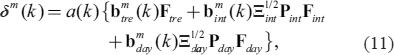
The set of SST perturbations represents the uncertainty of COBE-SST3, which is the sum of the errors in the low-frequency components (Fig. 7) and the analysis errors in the interannual variations and daily changes (Eq. 9). Here, we assumed that the sources of the uncertainty are independent among the three components. Uncertainties are large in areas with sparse data or of large background errors. Assuming that the EOFs used in the analysis can represent the truth with sufficient accuracy, the perturbations can be decomposed by the EOFs. The SST perturbation vector δm (k) for ensemble member m = (1, 2, …, M) at the k-th time step is given by
where bm is the normalized EOF score vector, and the Ξ and P are the eigenvalue and eigenvector matrices of (Λ−1 + Ft Ht R−1 HF)−1 in Eq. (9). Ξ is diagonal. Suffixes “tre,” “int,” and “day” stand for low-frequency component, interannual variation, daily change, respectively. Equation (11) provides a set of perturbations proportional to the analysis errors. For each perturbation component, the spreads of the perturbations and the corresponding analysis errors are comparable with each other. However, the spreads of δm(k) become smaller than the analysis errors, because the three components are independently given. Therefore, scalar a(k) was introduced to make the spread equivalent to the analysis error, which took values around 1.3. In Eq. 11, the error in the low-frequency components is given in a different style from the others, because the theoretical analysis errors for the low-frequency components were not available. Since the most part of the variance of the low-frequency components is explained by a couple of leading EOF modes, Ftre, the spread of  was adjusted to the error at each time step. Six EOF modes explaining 95 % of the low-frequency variability were used in this study.
The time series of m-th score vector bm is given by a first order autoregressive model:
where  is the weight, and ϵm contains white noise.
  is estimated from the score time series of detrended SST anomalies in the least squares sense. The value is less than and close to 1, which ensures that the bm(k) time series are not divergent. The independence between the perturbations relies on the randomness of ϵm, and therefore any ensemble size is possible.
The perturbed SSTs are finally provided by adding δm(k) to COBE-SST3. The perturbations of sea ice concentration (SIC) are computed consistently with the SST perturbations. The same SIC-SST relationship (Section 3.5) is used here.
A.5 SST bias computation
To obtain the SST observation biases as a function of the observation instruments, the variational minimization method (Section 3.2; Eq. 1) is used to compute the biases on an annual basis. The computed biases are spatially invariant. The bias corrections (x) for six methods are analyzed using the global mean differences in SSTs between unbiased and biased instruments and differences between biased SST observations and HadNMAT2 as observations (y). The error variances of the bias corrections, E, are set to (0.15K)2, where E is diagonal. The error variances for y, i.e., F, are given by αE, where α is the inverse of the fractional spatial coverage based on the 5° × 5° grid. In Section 3.2, two types of the differences are used: one is the difference between biased and unbiased observations, and the other is the difference between biased observations. The observation matrix H is simply 1 for the former case, while it becomes an operator that gives a difference in the corrections between the methods. y is constituted by the samples of these differences in consecutive five years centered at the year of the bias.
References
- Barnett, T. P., 1984: Long-term trends in surface temperature over the oceans. Mon. Wea. Rev., 112, 303–312.
- Boyer, T. P., J. I. Antonov, O. K. Baranova, C. Coleman, H. E. Garcia, A. Grodsky, D. R. Johnson, R. A. Locarnini, A. V. Mishonov, T. D. O’Brien, C. R. Paver, J. R. Reagan, D. Seidov, I. V. Smolyar, and M. M. Zweng, 2013: World ocean database 2013. NOAA Atlas NESDIS, No. 72, Levitus, S., and A. V. Mishonov (eds.), NOAA, 209 pp.
- Brönnimann, S., 2006: The global climate anomaly 1940–1942. Weather, 60, 336–342.
- Chan, D., and P. Huybers, 2019: Systematic differences in bucket sea surface temperature measurements among nations identified using a linear mixed-effect method. J. Climate, 32, 2569–2589.
- Chan, D., E. C. Kent, D. I. Berry, and P. Huybers, 2019: Correcting datasets leads to more homogeneous early-twentieth-century sea surface warming. Nature, 571, 393–397.
- Comiso, J. C., D. J. Cavalieri, C. L. Parkinson, and P. Gloersen, 1997: Passive microwave algorithms for sea ice concentration: A comparison of two technique. Remote Sens. Environ., 60, 357–384.
- Cornes, R. C., E. C. Kent, D. I. Berry, and J. J. Kennedy, 2020: CLASSnmat: A global night marine air temperature data set, 1880–2019. Geosci. Data J., 7, 170–184.
- Derber, J., and A. Rosati, 1989: A global oceanic data assimilation system. J. Phys. Oceanogr., 19, 1333–1347.
- Eyring, V., S. Bony, G. A. Meehl, C. A. Senior, B. Stevens, R. J. Stouffer, and K. E. Taylor, 2016: Overview of the Coupled Model Intercomparison Project Phase 6 (CMIP6) experimental design and organization. Geosci. Model Dev., 9, 1937–1958.
- Folland, C. K., and D. E. Parker, 1995: Correction of instrumental biases in historical sea surface temperature data. Quart. J. Roy. Meteor. Soc., 121, 319–367.
- Freeman, E., S. D. Woodruff, S. J. Worley, S. J. Lubker, E. C. Kent, W. E. Angel, D. I. Berry, P. Brohan, R. Eastman, L. Gates, W. Gloeden, Z. Ji, J. Lawrimore, N. A. Rayner, G. Rosenhagen, and S. R. Smith, 2017: ICOADS release 3.0: A major update to the historical marine climate record. Int. J. Climatol., 37, 2211–2232.
- Gandin, L. S., 1963: Objective Analysis of Meteorological Fields. Gidrometeorizdar, 238 pp (Translated from Russian by Israeli Program for Scientific Translations in 1965.) [Available at https://api.semanticscholar.org/CorpusID:127840621.]
- Ghil, M., and P. Malanotte-Rizzoli, 1991: Data assimilation in meteorology and oceanography. Advances in Geophysics. vol.33. Dmowska, R. (ed.), Academic Press, 141–266.
- Good, S. A., M. J. Martin, and N. A. Rayner, 2013: EN4: Quality controlled ocean temperature and salinity profiles and monthly objective analyses with uncertainty estimates. J. Geophys. Res.: Oceans, 118, 6704–6716.
- Gouretski, V., and F. Reseghetti, 2010: On depth and temperature biases in bathythermograph data: Development of a new correction scheme based on analysis of a global ocean database. Deep-Sea Res., 57, 812–833.
- Haarsma, R. J., M. J. Roberts, P. L. Vidale, C. A. Senior, A. Bellucci, Q. Bao, P. Chang, S. Corti, N. S. Fučkar, V. Guemas, J. von Hardenberg, W. Hazeleger, C. Kodama, T. Koenigk, L. R. Leung, J. Lu, J.-J. Luo, J. Mao, M. S. Mizielinski, R. Mizuta, P. Nobre, M. Satoh, E. Scoccimarro, T. Semmler, J. Small, and J.-S. von Storch, 2016: High resolution model intercomparison project (HighResMIP v1. 0) for CMIP6. Geosci. Model Dev., 9, 4185–4208.
- Hirahara, S., M. Ishii, and Y. Fukuda, 2014: Centennial-scale sea surface temperature analysis and its uncertainty. J. Climate, 27, 57–75.
- Huang, B., V. F. Banzon, E. Freeman, J. Lawrimore, W. Liu, T. C. Peterson, T. M. Smith, P. W. Thorne, S. D. Woodruff, and H.-M. Zhang, 2015: Extended reconstructed sea surface temperature version 4 (ERSST. v4). Part I: Upgrades and intercomparisons. J. Climate, 28, 911–930.
- Huang, B., P. W. Thorne, V. F. Banzon, T. Boyer, G. Chepurin, J. H. Lawrimore, M. J. Menne, T. M. Smith, R. S. Vose, and H.-M. Zhang, 2017: Extended reconstructed sea surface temperature, version 5 (ERSSTv5): Upgrades, validations, and intercomparisons. J. Climate, 30, 8179–8205.
- Huang, B., C. Liu, V. Banzon, E. Freeman, G. Graham, B. Hankins, T. Smith, and H.-M. Zhang, 2021: Improvements of the daily optimum interpolation sea surface temperature (DOISST) version 2.1. J. Climate, 34, 2923–2939.
- Ide, K., P. Courtier, M. Ghil, and A. C. Lorenc, 1997: Unified notation for data assimilation: Operational, sequential and variational (gtspecial issueltdata assimilation in meteology and oceanography: Theory and practice). J. Meteor. Soc. Japan, 75, 181–189.
- Ishii, M., and N. Mori, 2020: d4PDF: Large-ensemble and high-resolution climate simulations for global warming risk assessment. Prog. Earth Planet. Sci., 7, 58, doi:10.1186/s40645-020-00367-7.
- Ishii, M., M. Kimoto, and M. Kachi, 2003: Historical ocean subsurface temperature analysis with error estimates. Mon. Wea. Rev., 131, 51–73.
- Ishii, M., A. Shouji, S. Sugimoto, and T. Matsumoto, 2005: Objective analyses of sea-surface temperature and marine meteorological variables for the 20th century using ICOADS and the Kobe collection. Int. J. Climatol., 25, 865–879.
- Ishii, M., Y. Fukuda, S. Hirahara, S. Yasui, T. Suzuki, and K. Sato, 2017: Accuracy of global upper ocean heat content estimation expected from present observational data sets. SOLA, 13, 163–167.
- Ishii, M., H. Kamahori, H. Kubota, M. Zaiki, R. Mizuta, H. Kawase, M. Nosaka, H. Yoshimura, N. Oshima, E. Shindo, H. Koyama, M. Mori, S. Hirahara, Y. Imada, K. Yoshida, T. Nozawa, T. Takemi, T. Maki, and A. Nishimura, 2024: Global historical reanalysis with a 60-km AGCM and surface pressure observations: OCADA. J. Meteor. Soc. Japan, 102, 209–240.
- Jones, P. D., T. M. L. Wigley, and P. B. Wright, 1986: Global temperature variations between 1861 and 1984. Nature, 322, 430–434.
- Junod, R. A., and J. R. Christy, 2020: A new compilation of globally gridded night-time marine air temperatures: The UAHNMATv1 dataset. Int. J. Climatol., 40, 2609–2623.
- Kanda, T., 1962: On microfilm and puched card copies of marine meteorological observation records. Wea. Service Bull., 29, 109–116 (in Japanese).
- Kaplan, A., M. A. Cane, Y. Kushnir, A. C. Clement, M. B. Blumenthal, and B. Rajagopalan, 1998: Analyses of global sea surface temperature 1856–1991. J. Geophys. Res., 103, 18567–18589.
- Kennedy, J. J., N. A. Rayner, R. O. Smith, D. E. Parker, and M. Saunby, 2011: Reassessing biases and other uncertainties in sea-surface temperature observations measured in situ since 1850: 1. Measurement and sampling uncertainties. J. Geophys. Res., 116, D14103, doi:10.1029/2010JD015220.
- Kennedy, J. J., N. A. Rayner, C. P. Atkinson, and R. E. Killick, 2022: HadSST. 4.0.1.0 product user guide. Met Office, 35 pp. [Available at: https://www.metoffice.gov.uk/hadobs/hadsst4/HadSST.4.0.1.0_Product_User_Guide.pdf.]
- Kent, E. C., S. D. Woodruff, and D. I. Berry, 2007: Metadata from WMO publication no. 47 and an assessment of voluntary observing ship observation heights in ICOADS. J. Atmos. Oceanic Technol., 24, 214–234.
- Kent, E. C., J. J. Kennedy, D. I. Berry, and R. O. Smith, 2010: Effects of instrumentation changes on sea surface temperature measured in situ. WIREs Climate Change, 1, 718–728.
- Kent, E. C., N. A. Rayner, D. I. Berry, M. Saunby, B. I. Moat, J. J. Kennedy, and D. E. Parker, 2013: Global analysis of night marine air temperature and its uncertainty since 1880: The HadNMAT2 data set. J. Geophys. Res.: Atmos., 118, 1281–1298.
- Kobayashi, S., Y. Ota, Y. Harada, A. Ebita, M. Moriya, H. Onoda, K. Onogi, H. Kamahori, C. Kobayashi, H. Endo, K. Miyaoka, and K. Takahashi, 2015: The JRA-55 reanalysis: General specifications and basic characteristics. J. Meteor. Soc. Japan, 93, 5–48.
- Lenssen, N. J., G. A. Schmidt, J. E. Hansen, M. J. Menne, A. Persin, R. Ruedy, and D. Zyss, 2019: Improvements in the GISTEMP uncertainty model. J. Geophys. Res.: Atmos., 124, 6307–6326.
- Liu, C., E. Freeman, E. C. Kent, D. I. Berry, S. J. Worley, S. R. Smith, B. Huang, H.-m. Zhang, T. Cram, Z. Ji, M. Ouellet, I. Gaboury, F. Oliva, A. Andersson, W. E. Angel, A. R. Sallis, and A. Adeyeye, 2022: Blending TAC and BUFR marine in situ data for ICOADS near-real-time release 3.0.2. J. Atmos. Oceanic Technol., 39, 1943–1959.
- Menne, M. J., C. N. Williams, B. E. Gleason, J. J. Rennie, and J. H. Lawrimore, 2018: The global historical climatology network monthly temperature dataset, version 4. J. Climate, 31, 9835–9854.
- Meredith, M. P., and A. M. Hogg, 2006: Circumpolar response of Southern Ocean eddy activity to a change in the Southern Annular Mode. Geophys. Res. Lett., 33, L16608, doi:10.1029/2006GL026499.
- Mizuta, R., A. Murata, M. Ishii, H. Shiogama, K. Hibino, N. Mori, O. Arakawa, Y. Imada, K. Yoshida, T. Aoyagi, H. Kawase, M. Mori, Y. Okada, T. Shimura, T. Nagatomo, M. Ikeda, H. Endo, M. Nosaka, M. Arai, C. Takahashi, K. Tanaka, T. Takemi, Y. Tachikawa, K. Temur, Y. Kamae, M. Watanabe, H. Sasaki, A. Kitoh, I. Takayabu, E. Nakakita, and M. Kimoto, 2017: Over 5,000 years of ensemble future climate simulations by 60-km global and 20-km regional atmospheric models. Bull. Amer. Meteor. Soc., 98, 1383–1398.
- Noone, S., C. Atkinson, D. I. Berry, R. J. H. Dunn, E. Freeman, I. Perez Gonzalez, J. J. Kennedy, E. C. Kent, A. Kettle, S. McNeill, M. Menne, A. Stephens, P. W. Thorne, W. Tucker, C. Voces, and K. M. Willett, 2021: Progress towards a holistic land and marine surface meteorological database and a call for additional contributions. Geosci. Data J., 8, 103–120.
- Olonscheck, D., M. Rugenstein, and J. Marotzke, 2020: Broad consistency between observed and simulated trends in sea surface temperature patterns. Geophys. Res. Lett., 47, e2019GL086773, doi:10.1029/2019GL086773.
- Osborn, T. J., and P. D. Jones, 2014: The CRUTEM4 land-surface air temperature data set: Construction, previous versions and dissemination via Google Earth. Earth Syst. Sci. Data, 6, 61–68.
- Paltridge, G., and S. Woodruff, 1981: Changes in global surface temperature from 1880 to 1977 derived from historical records of sea surface temperature. Mon. Wea. Rev., 109, 2427–2434.
- Parker, D. E., C. K. Folland, and M. Jackson, 1995: Marine surface temperature: Observed variations and data requirements. Climatic Change, 31, 559–600.
- Rayner, N. A., D. E. Parker, E. B. Horton, C. K. Folland, L. V. Alexander, D. P. Rowell, E. C. Kent, and A. Kaplan, 2003: Global analyses of sea surface temperature, sea ice, and night marine air temperature since the late nineteenth century. J. Geophys. Res., 108, 4407, doi: 10.1029/2002JD002670.
- Rayner, N. A., P. Brohan, D. E. Parker, C. K. Folland, J. J. Kennedy, M. Vanicek, T. J. Ansell, and S. F. B. Tett, 2006: Improved analyses of changes and uncertainties in sea surface temperature measured in situ since the mid-nineteenth century: The HadSST2 dataset. J Climate, 19, 446–469.
- Reynolds, R.W., and D. B. Chelton, 2010: Comparisons of daily sea surface temperature analyses for 2007–08. J. Climate, 23, 3545–3562.
- Reynolds, R. W., T. M. Smith, C. Liu, D. B. Chelton, K. S. Casey, and M. G. Schlax, 2007: Daily high-resolution-blended analyses for sea surface temperature. J. Climate, 20, 5473–5496.
- Saha, K., X. Zhao, H.-m. Zhang, K. S. Casey, D. Zhang, S. Baker-Yeboah, K. A. Kilpatrick, R. H. Evans, T. Ryan, and J. M. Relph, 2018: AVHRR Pathfinder version 5.3 level 3 collated (L3C) global 4km sea surface temperature for 1981-Present. NOAA National Centers for Environmental Information, Asheville, NC, USA. [Available at https://www.ncei.noaa.gov/access/metadata/landing-page/bin/iso?id=gov.noaa.nodc:AVHRR_Pathfinder-NCEI-L3C-v5.3.] (Accessed on 1 June 2023).
- Slivinski, L. C., G. P. Compo, J. S. Whitaker, P. D. Sardeshmukh, B. S. Giese, C. McColl, R. Allan, X. Yin, R. Vose, H. Titchner, J. Kennedy, L. J. Spencer, L. Ashcroft, S. Brönnimann, M. Brunet, D. Camuffo, R. Cornes, T. A. Cram, R. Crouthamel, F. Domínguez-Castro, J. E. Freeman, J. Gergis, E. Hawkins, P. D. Jones, S. Jourdain, A. Kaplan, H. Kubota, F. L. Blancq, T.-C. Lee, A. Lorrey, J. Luterbacher, M. Maugeri, C. J. Mock, G. W. K. Moore, R. Przybylak, C. Pudmenzky, C. Reason, V. C. Slonosky, C. A. Smith, B. Tinz, B. Trewin, M. A. Valente, X. L. Wang, C. Wilkinson, K. Wood, and P. Wyszyński, 2019: Towards a more reliable historical reanalysis: Improvements for version 3 of the twentieth century reanalysis system. Quart. J. Roy. Meteor. Soc., 145, 2876–2908.
- Smith, T. M., and R. W. Reynolds, 2002: Bias corrections for historical sea surface temperatures based on marine air temperatures. J. Climate, 15, 73–87.
- Smith, T. M., and R. W. Reynolds, 2003: Extended reconstruction of global sea surface temperatures based on COADS data (1854–1997). J. Climate, 16, 1495–1510.
- Thorne, P. W., K. M. Willett, R. J. Allan, S. Bojinski, J. R. Christy, N. Fox, S. Gilbert, I. Jolliffe, J. J. Kennedy, E. Kent, A. K. Tank, J. Lawrimore, D. E. Parker, N. Rayner, A. Simmons, L. Song, P. A. Stott, and B. Trewin, 2011: Guiding the creation of a comprehensive surface temperature resource for twenty-first-century climate science. Bull. Amer. Meteor. Soc., 92, ES40–ES47.
- Walsh, J. E., and W. L. Chapman, 2001: 20th-Century sea-ice variations from observational data. Ann. Glaciol., 33, 444–448.
- Walsh, J. E., F. Fetterer, J. Scott Stewart, and W. L. Chapman, 2017: A database for depicting Arctic sea ice variations back to 1850. Geogr. Rev., 107, 89–107.
- Wentz, F. J., L. Ricciardulli, C. Gentemann, T. Meissner, K. A. Hilburn, and J. Scott, 2013: Remote sensing systems coriolis WindSat [Daily] environmental suite on 0.25 deg grid, version 7.0.1. [Available at https://www.remss.com/missions/windsat.] (Accessed on 1 June 2023).
- Wentz, F. J., T. Meissner, C. Gentemann, and M. Brewer, 2014a: Remote sensing systems AQUA AMSR-E [Daily] environmental suite on 0.25 deg grid, version 7. [Available at https://www.remss.com/missions/amsr.] (Accessed on 1 June 2023).
- Wentz, F. J., T. Meissner, C. Gentemann, K. A. Hilburn, and J. Scott, 2014b: Remote sensing systems GCOM-W1 AMSR2 [Daily] environmental suite on 0.25 deg grid, version 8.2. [Available at https://www.remss.com/missions/amsr.] (Accessed on 1 June 2023).
- Woodruff, S. D., R. J. Slutz, R. L. Jenne, and P. M. Steurer, 1987: A comprehensive ocean-atmosphere data set. Bull. Amer. Meteor. Soc., 68, 1239–1250.
- Woodruff, S. D., S. J. Worley, S. J. Lubker, Z. Ji, J. Eric Freeman, D. I. Berry, P. Brohan, E. C. Kent, R. W. Reynolds, S. R. Smith, and C. Wilkinson, 2011: ICOADS Release 2.5: Extensions and enhancements to the surface marine meteorological archive. Int. J. Climatol., 31, 951–967.
- Xie, S.-P., J. Hafner, Y. Tanimoto, W. T. Liu, H. Tokinaga, and H. Xu, 2002: Bathymetric effect on the winter sea surface temperature and climate of the Yellow and East China Seas. Geophys. Res. Lett., 29, 81-1–81-4.
- Yang, C., F. E. Leonelli, S. Marullo, V. Artale, H. Beggs, B. B. Nardelli, T. M. Chin, V. De Toma, S. Good, B. Huang, C. J. Merchant, T. Sakurai, R. Santoleri, J. Vazquez-Cuervo, H.-M. Zhang, and A. Pisano, 2021: Sea surface temperature intercomparison in the framework of the Copernicus Climate Change Service (C3S). J. Climate, 34, 5257–5283.
- Yasuda, I., 2003: Hydrographic structure and variability in the Kuroshio-Oyashio transition area. J. Oceanogr., 59, 389–402.