Abstract
Improving the existing limited network of observation sites and quantifying carbonyl sulfide (COS) temporal variability allows a more accurate understanding of the COS budget. A system with low-power consumption would enable COS concentration measurements at various observation sites. Therefore, we designed a continuous measurement system employing a commercially available portable laser-based analyser to measure atmospheric COS concentrations. To obtain precise atmospheric COS concentrations, (1) the temperature of the optical cell was stabilised at 0.13 ± 0.014 °C h−1 using double insulation with a refrigerator and insulation material, (2) ambient air was used as a reference gas for 30 s every minute (1 cycle min−1) after reducing its COS level to below 100 ppt using activated charcoal, and (3) the difference in water vapour concentration between ambient air and the reference was maintained within ± 400 ppm. The ambient COS concentrations were determined using three calibration gases with known COS concentrations prepared by the National Oceanic and Atmospheric Administration (NOAA). The analytical precision of the system was 12.1 ppt (1σ) over a 15-min, allowing for sufficient characterisation of diurnal variations of the atmospheric COS concentration. The observation in Tsukuba, Japan, showed that the observed COS concentrations in April 2023 were 410–599 ppt. Backward trajectory analysis revealed that air masses with high COS concentrations exceeding 550 ppt traversed over the Keihin Industrial Zone. This suggests that a continuous measurement system may discover potential COS sources, helping establish a COS observing network for more accurate oceanic and anthropogenic flux measurements.
1. Introduction
Carbonyl sulfide (COS or OCS) is the most abundant sulfur-containing gas in the ambient atmosphere, with an average concentration of approximately 500 parts per trillion (ppt) in the troposphere (Chin and Davis 1995; Montzka et al. 2007). Because of its long lifetime (more than two years), COS is converted to stratospheric sulfate aerosols (SSA) in the stratosphere (Crutzen 1976), affecting the Earth’s radiation balance and contributing to ozone depletion. Furthermore, COS has been suggested as a potential tracer of gross primary production (GPP) because of its similar uptake mechanism into plants through the stomata as part of photosynthesis processes of carbon dioxide (CO2), whereas COS is not re-emitted to the atmosphere as CO2 in respiration processes (Campbell et al. 2008).
Identifying sources and sinks and characterizing the spatial-temporal distribution of COS concentrations will help to elucidate its contribution to SSA and its role as a tracer for global GPP. COS in the atmosphere primarily originates from oceanic and anthropogenic sources. Emissions from the ocean include direct and indirect COS sources (Kettle et al. 2002; Berry et al. 2013). Indirect oceanic COS emissions are caused by the oxidation of emitted carbon disulfide (CS2) and dimethyl sulfide (DMS) (Berry et al. 2013; Li et al. 2024). Anthropogenic COS sources include direct and indirect emissions from the oxidation of emitted CS2. The dominant anthropogenic source is rayon production (Campbell et al. 2015), while other large sources include aluminium production, coal combustion, oil refineries, and fuel combustion (Chin and Davis 1995; Zumkehr et al. 2018). The main contributors to the COS sinks in the troposphere are terrestrial vegetation and soil uptakes (Montzka et al. 2007). Minor contributions to COS sinks include photolysis and reactions with hydroxyl radical and oxygen atoms [O(3P)] are also considered (Kettle et al. 2002; Chin and Davis 1995; Li et al. 2024).
The global spatial-temporal distribution of the COS concentration is monitored by a global monitoring network managed by the National Oceanic and Atmospheric Administration (NOAA) based on flask samples shipped to the laboratory for analysis using gas chromatography–mass spectrometry (GC–MS) (Montzka et al. 2007). This method can be applied in remote locations but has limited time resolution. Since 2010, in situ COS concentration measurements using laser spectroscopy have been reported. A quantum cascade laser spectrometer (Aerodyne Research Inc., Billerica, USA) and a COS analyser using off-axis integrated cavity output spectroscopy (ABB-Los Gatos Research, Zurich, Switzerland) provided high-frequency (> 1 Hz) COS and CO2 concentration measurements (Stimler et al. 2010a, b; Commane et al. 2013; Berkelhammer et al. 2014; Kooijmans et al. 2016; Belviso et al. 2016, 2020; Rastogi et al. 2018; Zanchetta et al. 2023). These COS concentration analysers enabled high-resolution COS concentration measurements, revealing diurnal variations in COS concentrations and fluxes in forested areas and soils. Furthermore, satellite observations and models have improved our understanding of the spatial and temporal distributions of COS sources and sinks (Kuai et al. 2015; Glatthor et al. 2017; Ma et al. 2023; von Hobe et al. 2023). However, oceanic and anthropogenic COS fluxes remain uncertain, and there remains significant gaps between bottom-up estimates of sources and sinks (Berry et al. 2013; Whelan et al. 2018; Berchat et al. 2024). To obtain precise spatial-temporal variations in COS fluxes, establishing a network of observation sites, such as the Integrated Carbon Observatory System (ICOS, Hazan et al. 2016), is required (Berchat et al. 2024). Because COS emissions from anthropogenic and marine sources can show diurnal variations (Berkelhammer et al. 2016; Berchat et al. 2024), continuous COS concentration measurements are necessary to better understand these emissions. However, the high cost, weight (over 35 kg), and power consumption (over 400 W) of these laser COS instruments limit their setup at additional observation sites.
In this study, we designed a continuous measurement system for observing the atmospheric COS concentration using a commercially available portable laser-based analyser. The power consumption and cost of our continuous measurement system were notably lower than those employing previously reported COS analysers (Stimler et al. 2010a, b; Commane et al. 2013; Kooijmans et al. 2016; Rastogi et al. 2018; Belviso et al. 2020; Zanchetta et al. 2023). Section 2 describes the designed system. Section 3 presents the results of performance test results of the system. Section 4 provides a detailed description of the field measurements conducted using the system.
2. Experimental setup
2.1 System configuration
The continuous measurement system designed in this study for atmospheric COS concentration measurement is schematically illustrated in Fig. 1. The system consists of a portable laser-based analyser (MIRA Pico analyser; Aeris Technologies, CA, USA) and a gas handling system. The analyser outputs the COS and CO2 signals by referencing their spectra to the peak positions of the water spectrum in the approximately 4 µm region, and the COS and CO2 spectra were fitted separately. Therefore, sample air must contain a certain level of the water vapour concentration (> 1,000 ppm), making it challenging to measure in low-humidity environments such as polar and high-altitude regions. The output COS signal is in the dry mole fraction with a 1-point linear correction determined by the manufacturer. The analyser has two inlets that switch sample and reference gases by a three-port solenoid valve to reduce the signal drift owing to changes in temperature and water vapour concentration in the optical cell. In this study, the optical cell package was detached from the original analyser case and placed in a small refrigerator to stabilise the cell temperature (see below).

The gas handling system continuously introduced sample and reference gases into the portable laser-based analyser. Air was pumped by a Teflon-coated diaphragm pump (D-79112, KNF, Freiburg, Germany) to a Tee union through a 7-µm stainless steel filter (SS-4TF-7, Swagelok, State of Ohio, USA) (Filter_1). The Tee union split air into the sample and reference lines (Fig. 1). The sample line passed a 10-port multiposition valve, an electric cooler unit (ECU) (ECU_1) set at 2 °C, and the outer tubing of the Nafion dryer (MD-110-96S; Perma Pure LLC, NJ, USA), into port 0 of the portable laser-based analyser. The reference line passed through an ECU_2 set at 2 °C, activated charcoal in 215 mL tube with acrylic body and polyvinyl chloride end caps (IACH-50-200-215-CC; United Filtration System, Michigan, USA), and the Nafion dryer, and then was introduced into port 1 of the analyser. The ECU and Teflon-coated pump were do not affect the measurement of COS concentrations in the air (see Supplement 1). The ECU and Nafion dryer were used to control the water vapour concentration. The ECU prevents air with a high water vapour concentration from being introduced into the optical cell, which could cause condensation on the mirror surface. The ECU and Nafion dryer also increase the humidity of the dry air. The ECU, equipped with a Peltier cooler, facilitated air cooling and disposal of condensed water into the drain. The positive pressure in the ECU forced the accumulated water and air to be expelled through the bottom port of the ECU. The bottom port is normally 1/8 inch in diameter, but a tube with an outer diameter of 1/16 inch was connected to the port to reduce air consumption. Consequently, water droplets were retained in the ECU owing to the infrequent draining of water from the ECU, allowing the dry air passing through the ECU to be humidified by the retained water. Humidification from the ECU also enabled the measurement of the COS signal in dry air. The Nafion dryer facilitates the transfer of water molecules from a gas with a high water vapour concentration to a gas with a low water vapour concentration via a Nafion membrane. To reduce water vapour in the sample gas, dry air is typically used in countercurrent flow; however, the parallel flow was used in this study to maintain similar water vapour concentrations in the sample gas (H2Osam) and reference gas (H2Oref). To measure precise COS concentrations, reducing the difference in the water vapour concentration between the sample and reference gases using a Nafion dryer is important (see Section 3.2). The activated charcoal removed most of the COS in the reference gas (see details in Section 3.3). Dehumidified air was expelled through vent lines at over 50 mL min−1 to introduce either sample or reference gas into the portable laser-based analyser at atmospheric pressure.
In the portable laser-based analyser, the air sampled through the inlets was filtered with a 0.01 micron fluorocarbon borosilicate glass microfiber element (Filter_2). Then, the air entered the optical cell through a flow regulation valve. The air passing through the optical cell was exhausted through a mini-pump. The flow regulation valve controlled the pressure in the optical cell to 14,000 Pa (140 mbar) by feedback of voltage according to the pressure in the cell. The flow rate was regulated through the mini-pump voltage and was set at approximately 210 mL min−1 for this study, with a possible range from approximately 160 mL min−1 to 260 mL min−1. An increased flow rate reduced gas exchange time, but the shortens the lifespan of the mini-pump. The minimum total flow rate required for the sample or reference line was ≥ 300 mL min−1 because some air was exhausted from the vent line and ECU. During atmospheric observations, air flowed into the sample and reference lines at 750 mL min−1, but more than 400 mL min−1 was released through the vent.
The temperature inside the cell was stabilised using a Peltier cooler and a refrigerator. This is because the temperature stability of the cell is important for improving the analytical precision of COS concentration measurements (see Section 3.1). The cell package containing two circuit boards, a laser, and an optical cell with a detector was surrounded by thermal insulation material, which is an aerogel sheet on blue Styrofoam, and the temperature was controlled by a Peltier cooler set at 29 °C placed under the optical cell. The Peltier cooler dissipated the heat from the optical cell into the inside of the refrigerator (FCI-280G, AS ONE Corporation, Osaka, Japan), which was set at 15 °C (Fig. 1). The refrigerator transferred the heat from the Peltier cooler to the outside.
The output data from the system was saved on an SD card in the computer integrated into the portable laser analyser. The data were copied to our microcomputer (Raspberry Pi, Raspberry Pi Ltd, Cambridge, UK) and transmitted over the Internet to our server. Portable laser-based analysers and continuous measurement systems often encounter weekly errors, requiring a reboot that is not feasible remotely. Although several types of errors can occur, the most common is that the cessation of flow path switching. It may also cause the loss of the water peak or the measurement to stop working. The cause of these errors is unknown; however, we believe that they may be due to excessive demands on the computer’s processing power. To address this, a relay was used to simulate the power button being pressed for daily automatic restarts via a microcomputer command. This minimised data loss from system failures. Considering that the temperature and laser output were not stable immediately after rebooting, the data from 30 min to 1 h after rebooting was discarded.
The continuous measurement system designed in this study uses 150 W, weighs 10 kg, and can be installed in a 50 × 80 × 60 cm space. Therefore, this system is lightweight, affordable, and energy efficient compared with those reported by past studies (Stimler et al. 2010a, b; Commane et al. 2013; Kooijmans et al. 2016; Belviso et al. 2016, 2020; Rastogi et al. 2018; Zanchetta et al. 2023). Consequently, it is suitable for on-site observations of atmospheric COS concentration.
2.2 Measurement procedures of COS concentration
Figure 2 shows an example of the output COS signal from the portable laser-based analyser of the continuous measurement system obtained during actual atmospheric observations at approximately 1 Hz. As described above, to cancel the signal drifts of the analyser, the two inlets were switched between the sample and reference gases every 30 s. Based on the data indicating that it took approximately 8 s to replace the air in the cell, the COS signals during the first 10 s after switching were excluded. Then, a corrected COS value (hereafter referred to as “COSsam-ref_corrected2”) was calculated using the following Equations.

The COSsam and COSref represent the COS signals of the sample and reference gases, respectively, measured by a portable laser-based analyser. The COSsam-ref value was calculated by the difference of the COSsam from the average of the preceding and following COSref values. Furthermore, the COSsam-ref_corrected values were corrected to account for the difference between the H2Oref and H2Osam, and COSsam-ref_corrected2 values were corrected for the H2Osam (see Sections 3.2 and 3.3c). The corrected COSsam-ref_corrected2 values were converted to COS concentrations using three calibration gases as reference points. The calibration gases (cylinders A–C) are described in Section 2.3. To provide daily calibration lines, air from cylinder A was introduced through the sample line via the 10-port multiposition valve for 10 min, followed by 2 min of ambient air, 10 min of air from cylinder B, 2 min of ambient air, and 10 min of air from cylinder C. The intermediate ambient air through the multiposition valve for 2 min humidified the sample line before introducing of air from cylinders B and C. Alternatively, the dry air flow reduces the H2Osam, increasing the difference between the H2Osam and H2Oref. A large difference between the H2Osam and H2Oref affects the measurement of the COS concentration (see Section 3.2). The COSsam-ref_corrected2 values from the last 5 min of the 10 min analysis were averaged to represent the value for each calibration gas. Figure 3 shows an example of the relationships between the COSsam-ref_corrected2 values and COS concentrations in the calibration gases from 12–21 April 2023. The calibration line in Fig. 3a represents the Deming least-square fit, and the coefficient of determination (R2-value) was 0.98. Figure 3b shows the residuals of the COSsam-ref_corrected2 value from the line, and the average of residuals was −2.9, 5.3, and −2.4 ppt of air from cylinders A, B, and C, respectively. The residuals of the COSsam-ref_corrected2 value were within the range of 5-min analytical precision (see Section 3.4). Therefore, the calibration line was straight in the COS concentration range of calibration gas (360–565 ppt). For atmospheric observations, COS concentrations were determined by time interpolation using daily calibration lines.

A total of seven high-pressure air cylinders were used in this study (Table 1). The air in all cylinders was dehumidified. The calibration gases were ambient air filled with high pressure in Aculife IV treated aluminium cylinders at NOAA/Earth System Research Laboratories (ESRL). The calibration gas cylinders used in this study were named cylinders A, B, and C. The COS concentrations of calibration gases were determined on the NOAA-2004 COS scale at NOAA/ESRL based on the GC–MS measurements developed by Montzka et al. (2004) (Table 1). Although calibration gas provided by NOAA is widely used in the COS community, it is revealed that COS concentrations in these high-pressure cylinders of actual air can change significantly over time (COSANOVA HP: https://www.cosanova.org/calibration-gas.html). Because the use of a single calibration gas cannot detect changes in COS concentration, this study employed three calibration gases to continuously verify the linearity of the calibration line. If the coefficient of determination (R2-value) for the calibration line generated for the three gases exceeded 0.95, the calibration line was used on the assumption that the concentration of the NOAA gas remained stable. Dry ambient air was filled into two electropolished aluminium cylinders and one manganese steel cylinder to perform continuous flow experiments such as repeatability tests. These compressed air cylinders were called cylinders D, E, and F, respectively (Table 1). To verify the COS removal efficiency by activated charcoal, a manganese steel cylinder filled with synthetic air (COS-free air) was used as cylinder G (Table 1).

3. Performance of the continuous measurement system
This section describes the temperature stabilisation, differences between the H2Osam and H2Oref, and reference gas production using activated charcoal. These were tested to achieve highly precise and long-term continuous COS concentration measurements. We also evaluated the analytical precision of the system.
3.1 Temperature stabilisation
In similar portable laser-based analysers, which were used to measure formaldehyde concentrations, temperature instability significantly impacted the analytical precision determined by the Allan deviation (Mouat et al. 2024). To examine the relationship between the COSsam and temperature, air from cylinder B was introduced via port 0 of the original portable laser-based analyser for approximately 3.5 h via the multiposition valve of the sample line of the continuous measurement system for approximately 22 h. The COSsam were measured at 1 Hz (without switching) to eliminate the effects of reference gas stability and switching of ports.
Figure 4 shows typical temporal variations in the optical cell temperature and the output COSsam from the original portable laser-based analyser (Figs. 4a–c) and the continuous measurement system (Figs. 4d–f). For the former measurement, the temperature of the optical cell was 33.25 ± 0.34 °C (± 1σ), and it changed at 0.53 ± 0.56 °C h−1 (Fig. 4a). The COSsam from the analyser was 443 ± 1700 ppt for the period and correlated with the cell temperature (Fig. 4b). To examine the drift of the COSsam, the data points were hypothetically regarded as sample and reference at 30 s intervals. The COSsam-ref values were then calculated to determine the COS concentrations using the calibration line, which resulted in the COS concentration of 1.4 ± 43 ppt (Fig. 4c). In contrast, when the optical cell temperature was stabilised in the newly established system, the average temperature of the optical cell and COSsam from the COS analyser were more stable at 25.41 ± 0.08 °C and 4551 ± 576 ppt, respectively (Figs. 4d, e). The temperature of the optical cell changed at 0.13 ± 0.014 °C h−1. The COS concentrations measured by the continuous measurement system was −0.4 ± 25 ppt (Fig. 4f).

To diagnose the optimum sample-reference switching time with the least drift effect, we present the Allan variance plots for the portable laser-based analyser and the continuous measurement system. The Allan deviation plots effectively assess laser stability and show how much the noise level can be reduced by integration and when scale drift effects begin to occur (Allan 1987). The Allan variance (σ2) plots of the portable laser-based analyser and the continuous measurement system are shown in Fig. 5. In the Allan variance plot, the lowest value of Allan variance represents the most stable integration time, while white noise, nonlinear drift, and linear drift are represented by the slopes shown in Fig 5. The original portable laser-based analyser was dominated by white noise up to an integration time of 5 s and started to drift approximately non-linearly manner after approximately 30 s. The Allan variance was the smallest at 5 s, with a value of 680 ppt2 (26 ppt for 1σ) for the analyser. The continuous measurement system exhibited white noise for up to 20 s and started to drift approximately non-linearly after approximately 40 s. The Allan variance was the smallest at 40 s, with a value of 274 ppt2 (17 ppt for 1σ) for the system. For integration times of less than 5 s, the continuous measurement system had a higher Allan variance than the portable laser-based analyser, and for integration times of more than 10 s, the continuous measurement system had a lower Allan variance than the portable laser-based analyser. The increase in white noise in the continuous measurement system was considered due to vibrations from the refrigerator, fan, or the effects of cable extensions for integration times of less than 5 s. In comparison, the decrease in drift effects in the continuous measurement system was attributed to the stabilisation of the temperature of the optical cell for integration times of more than 10 s.

Based on the Allan variance plot results, to measure COS concentration precisely, the COS signal was integrated for 5–10 s, and 30–40 s, for the original portable laser-based analyser and the continuous measurement system, respectively. However, switching every 5–10 s did not stabilise the COS signal, whereas switching every 30 s allowed sufficient time for the COS signal to stabilise (Fig. 2). Consequently, the continuous measurement system is less susceptible to drift than a portable laser-based analyser. The data collected 10 s after switching were disregarded to ensure data stability, after which the reference was measured for 20 s, giving a 1-min cycle for the COS concentration measurement of the system.
3.2 Differences between the H2Oref and H2Osam
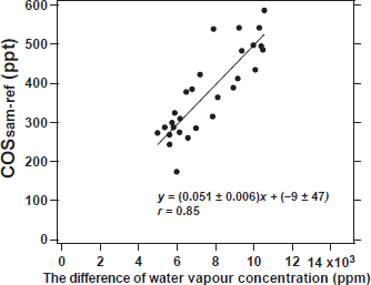
Evaluating the effect of water vapour concentration on gas concentration analysis is important because water vapour concentration dilutes the sample gas and generally affects the determination of gas concentrations in absorption spectroscopy (Kooijmans et al. 2016). We evaluated the effect of the difference between the H2Oref and H2Osam on the COS concentration measurement by the portable laser-based analyser without ECU and Nafion dryer. Air from cylinder B was used as the sample gas and connected to the original portable laser-based analyser. Synthetic air from cylinder G, humidified by passing it through a Nalgene bottle filled with water, was used as the reference gas and connected to the original portable laser-based analyser. The 250 mL Nalgene bottle containing 50 mL of water had two holes drilled on the top through which an air inlet and outlet tube were threaded and secured such that they would not contact the water in the bottle. The experiment was conducted as follows. In the first half, the sample gas was dry air from cylinder B. In the second half, air from cylinder B was humidified with sample gas by passing it through another Nalgene bottle containing water. The differences between the H2Oref and H2Osam on the COS concentration measurement using the portable laser-based analyser are shown in Fig. 6. Despite the temperature in the cell being maintained within 0.15 °C, the COSsam-ref values increased as the difference between the H2Oref and H2Osam increased. Figure 7 shows the relationship difference between the H2Oref and H2Osam and the COSsam-ref values. The correlation between the COSsam-ref values and difference the H2Oref and H2Osam infers a linear relationship with a slope of 0.05 ppt ppm−1 using the least squares method (r = 0.85, p-value < 0.05) (Fig. 7). Therefore, the difference between the H2Oref and H2Osam should be minimised to obtain accurate the COSsam-ref values.

As described in Section 3.1, the introduction of a reference gas at proper intervals is important to minimise the effect of the drift in measuring atmospheric COS concentration. However, synthetic air filled in a 47 L high-pressure cylinder would deplete within 16 d at a flow rate of 300 mL min−1. Frequent replacement of the cylinder is undesirable as it restricts the long-term operation of the measurement system. To avoid high consumption of synthetic air, we examine the use of ambient air combined with activated charcoal for the reference gas in the sections below. The following experiments were conducted to confirm that activated charcoal could be used to generate a reference gas.
a. COS removal efficiency
To estimate the COS removal efficiency in air by activated charcoal, ambient air and synthetic air from cylinder G were used as reference gases to compare COS concentrations of air from cylinders A–C. Air from cylinders A–C was introduced for 10 min each through the multiposition valve of the sample line. As a reference gas, the ambient air was pumped into the reference line or cylinder G was connected to a disconnected Tee in the gas handling system. The activated charcoal used in the experiment was used for one year. The COS signal value for the last 5 min was used for each calibration gas.
The results of adding air from cylinders A, B, and C to ambient air and air from cylinder G were defined using subscripts as follows: COSsam-ref, ambient air (= COSsam – COSref, ambient air) and COSsam-ref, cylinder G (= COSsam – COSref, cylinder G), respectively. Compared to the COSsam-ref, ambient air and COSsam-ref, cylinder G, the COSsam-ref, cylinder G values were 77 ± 18, 75 ± 30, 83 ± 21 ppt (1-min average and standard deviation) higher than the COSsam-ref, ambient air of air from cylinders A, B, and C, respectively. This suggests that the passage of air with COS concentrations typically observed in the atmosphere through activated charcoal removes only approximately 80 % of the COS. Note that this removal efficiency may vary depending on COS concentration. We note later that the degree of degradation of the activated charcoal may have influenced the COS removal efficiency (see Section 3.3d). However, since the COS concentration in air passed through activated charcoal is stable, it may be possible to use air with commonly observed COS concentrations passed through activated charcoal as a reference gas.
b. Effect of fluctuations in atmospheric COS concentration on reference gas generation
To investigate the dependence of COS removal efficiency on the COS concentration in the gas for the reference line, cylinders A–C were connected to the reference line from the disconnected Tee. Air from cylinders D and E were analysed via the sample line with a Nalgene bottle containing water introduced into the analyser for 20 min, followed by the second set of measurements. The 40 min (40 plots) data was grouped into 10-min sub-data to calculate the average and standard deviation of COS concentrations.
The average COS concentrations were calculated to be 638 ± 2, 634 ± 9, and 637 ± 1 ppt of air from cylinder D and 439 ± 9, 423 ± 20, and 429 ± 17 ppt of air from cylinder E, respectively, using reference gases produced from cylinders A, B, and C. A correlation test was performed on the relationship between the COS concentration of the air in cylinders D and F and the respective concentration of the reference gas, but the results showed no significant difference. Therefore, we conclude that the COS concentration in the reference gas downstream of the activated charcoal is almost constant regardless of upstream variations of the COS concentration in the ambient air (< 200 ppt).
When the reference gas is produced from ambient air, the variation of the COS concentration in the actual air may affect the calibration lines. To evaluate the variation of the calibration gas in the measurement of COS concentration, air from cylinders A–C was introduced at 15:00 and 21:00 and the following day at 3:00, 9:00, and 15:00 (JST).
Figure 8 shows the COSsam-ref_corrected2 values of air from cylinders A, B, and C and COS concentrations in the ambient air. The average and standard deviations (1σ) of the COSsam-ref_corrected2 values of air from cylinders A, B, and C were 345 ± 6, 439 ± 9, and 533 ± 9 ppt, respectively (Fig. 8a). The COS concentration in ambient air is shown in Fig, 8b. The COS concentrations were determined using the calibration lines constructed by analysing calibrating gases at different times, as described above. The red line represents the COS concentration as determined by the time interpolation of the calibration line. The standard deviation of the difference between the COS concentrations, calculated from the five calibration lines, was ± 7 ppt. Therefore, the choice of any calibration line within a day influenced the COS concentration measurement by no more than the standard deviation of the COSsam-ref_corrected2 value despite variation in the ambient air COS concentration exceeding 100 ppt (Fig. 8b). This suggests that reference gas generation from ambient air with activated charcoal is a practical solution for atmospheric observation and that measurement of a series of the calibration gas once a daily is sufficient.

To evaluate the long-term stability of the COS concentration measurements, the set of the calibration gases were analysed once daily from April to September without replacing the activated charcoal. The COSsam-ref_corrected values of the calibration gases for the period are shown in Fig. 9a. The average and standard deviation of the COSsam-ref_corrected value from April to September were 316 ± 19, 402 ± 17, and 495 ± 16 ppt for air from cylinders A, B, and C, respectively. These COSsam-ref_corrected values for the calibration gases showed no significant trends. Regression analysis was performed on the COSsam-ref_corrected value of each calibration gas versus time. The R2-values of the constructed calibration lines were always exceeded 0.95, except for two of the 102. As the three calibration gases maintained a linear relationship over the five-month period, the COS concentrations in the calibration gases unlikely changed during this period. The apparent H2Osam versus time are shown in Fig. 9b. The calibration gas was initially dry air but was subsequently humidified by passing through the ECU. Consequently, the H2Osam did not reflect the actual ambient air conditions. The apparent H2Osam when the calibration gas was pumped during the measurement period ranged from 4720 ppm to 13094 ppm from April to September 2023, and the average and standard deviation (1σ) of apparent H2Osam for humidified air from cylinders A, B, and C were 9856 ± 1641, 9469 ± 1439, and 9056 ± 1420 ppm, respectively. The coefficient of determination of the calibration line was not affected, but a change in the stability of the H2Osam before and after mid-June was observed. This variation was probably because water vapour entered the activated charcoal and measurement line during the shutdown period of the equipment, and the ECU could not control the H2Osam. For reference, water vapour concentrations at the Tateno site, 1 km east of the National Institute of Advanced Industrial Science and Technology (AIST) in Tsukuba, ranged from 2,000 ppm to 23,000 ppm from April to September 2023. When the water vapour concentration in the ambient air was low, the ECU humidified the ambient air to the apparent value of > 4720 ppm (Fig. 9). Conversely, when the ambient air had a high water vapour concentration, it was dehumidified down to 14,000 ppm or lower by the ECU.

Figure 10 shows the relationship between the COSsam-ref_corrected value and apparent H2Osam. The slopes of the COSsam-ref_corrected value and apparent H2Osam of air from cylinders A, B, and C, were 0.0041 ± 0.0011, 0.0045 ± 0.0011, and 0.0036 ± 0.0010 ppt ppm−1, respectively (Fig. 10), with an average of 0.0041 ± 0.0011 ppt ppm−1. The corresponding correlation coefficients were 0.35, 0.38, and 0.33 for air from cylinders A, B, and C, respectively. There are two possible reasons for the correlation between the COSsam-ref_corrected values and H2Osam: (1) spectroscopic effects that affect the absorption spectrum (enhanced pressure broadening or direct spectral interfering) and (2) the effect of dilution of the sample gas (Kooijman et al. 2016). As the COSsam-ref_corrected value and H2Osam were positively correlated, (2) the effect of dilution of the sample gas was unlikely. Conversely, the small spectrum of water may have interfered with the COS spectrum.

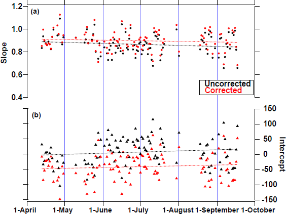
Because the calibration line is used to determine the COS concentration, we also verified that the calibration line was unchanged. The slope and intercept of the daily calibration line over a 5-month period, with and without correction from the H2Osam, are shown in Fig. 11. The apparent H2Osam was corrected by subtracting the H2Osam multiplied by 0.0041, 0.0045, and 0.0036 from the COSsam-ref_corrected values of air from cylinders A, B, and C, respectively. The calibration line for the period was defined as COS concentration = (0.86 ± 0.09) × COSsam-ref_corrected + (12 ± 45) for no correction (R2 = 0.994), whereas that for the corrected case it was COS concentration = (0.89 ± 0.09) × COSsam-ref_corrected + (−36 ± 44) (R2 = 0.995). The changes in the slope of the calibration line regarding time were −0.00025 ± 0.0002 for uncorrected and −0.00013 ± 0.0002 d−1 for corrected by H2Osam. The changes in the intercept of the calibration line regarding time were 0.09 ± 0.10 for uncorrected and 0.06 ± 0.09 d−1 for corrected by apparent H2Osam. The calibration line did not change significantly, regardless of the H2Osam. Therefore, the calibration line did not change over the 5-month period. However, when the H2Osam changed by 1,000 ppm, the COSsam-ref_corrected value was approximately 4.1 ppt higher (Fig. 10). To obtain more accurate values, the COSsam-ref_corrected2 value was used to determine the COS concentration.
No evident trends were observed over the 5-month period, but degradation of the activated charcoal may adversely affect the long-term observation. We evaluated how the “age” of activated charcoal influence the COS concentration measurement using the new and two-year-old materials. The COSsam-ref_corrected2 values of air from cylinders A–C were measured relative to ambient air with used or new activated charcoal. The test was conducted within two days.
The COSsam-ref values for air from cylinders A, B, and C were 251 ± 14, 347 ± 13, and 420 ± 9 ppt for the used activated charcoal, respectively, whereas, for the new activated charcoal, the values were 347 ± 2, 440 ± 4, and 540 ± 1 ppt, respectively. The slope and R2-values of calibration lines were 0.82 and 0.98 for the used activated charcoal and 0.94 and 1.00 for the new activated ones, respectively. The apparent H2Osam of air from cylinders A, B, and C were 7308 ± 272, 7755 ± 44, and 7633 ± 109 ppm for the used activated charcoal, and 8820 ± 373, 9497 ± 423, and 9593 ± 525 ppm for the new activated charcoal, respectively. The COSsam-ref_corrected2 values in the calibration gas were higher and varied less for the new activated charcoal than for the used activated one.
The difference in the COSsam-ref_corrected2 value can be attributed to the following three factors: (1) a decrease in the adsorption efficiency of activated charcoal, (2) an effect of H2Osam, and (3) a change in the sensitivity of the system. The second is unlikely because an increase in H2Osam of approximately 2,000 ppm would not increase the output of the COSsam-ref_corrected2 value by more than 10 ppt (see Section 3.3c). Furthermore, the third is also unlikely because this experiment was conducted within two days. Therefore, the decline in the COSsam-ref_corrected2 value is attributed to the decreased adsorption efficiency of activated charcoal. Because the activated charcoal itself is unlikely to change, the decrease in adsorption efficiency is possibly because of a decrease in the surface area of the activated charcoal that can adsorb gas. If activated charcoal were used for over two years, the slope of the calibration line using air from cylinders A, B, and C would decrease by approximately 20 % due to decrease in adsorption efficiency of the activated charcoal. However, the R2-value was higher than 0.95, and the calibration line remained linear over the COS concentration range of 360–565 ppt for used and new activated charcoal. The mechanism by which the used activated charcoal can also be utilised to generate a calibration line can be considered as follows. Activated charcoal traps volatile organic compounds (VOCs), and the concentration of VOCs in the air are much higher than those in COS (Bahlmann et al. 2011). Consequently, the adsorption efficiency of COS decreases as VOCs occupy the adsorption sites of the activated charcoal, resulting in a decreased slope of the calibration line produced by the COS calibration gas. However, the surface area of activated charcoal is approximately 400,000 m2 for 200 g to 300 g of activated charcoal (Cao et al. 2006), which is a substantial value for the molecule size. Even if a total of 10 L of air is passed through the activated charcoal for 40 min when the daily calibration line was generated, almost no effect on the occupancy rate of the activated charcoal was observed because the VOCs in the air were below the ppm level. Therefore, measuring the COS concentration using a calibration gas is possible, even though the reference gas is generated by passing air through the used activated charcoal. Although quantitative conclusions cannot be established in this context, replacing the filter annually in cases where the 1σ value is notably large is recommended.
3.4 Evaluation of analytical precision
We evaluated the repeatability of our measurement system and determined the COS concentration of the sample gas from a high-pressure cylinder for over a 24-h period. COS concentrations of air from cylinders D or F were measured to estimate the repeatability. In this experiment, air from cylinders D and F passed through a mass flow controller, a Nalgene bottle containing water and the multiposition valve of the sample line. Ambient air with activated charcoal was used as a reference gas.
Figure 12 shows the COS concentrations of air from cylinders D and F. The standard deviations of the 5-min average of COS concentrations were 19.7 ppt and 16.4 ppt, for air from cylinders D, and F, respectively. To characterise diurnal variations in the COS concentration with magnitude of 30–50 ppt (Berkelhammer et al. 2014), a measurement precision of 15 ppt or better is required. The systematic errors owing to the water vapour concentrations were corrected. We assumed that the analytical precision was only affected by random components.
The analytical precision (σtotal) derived from the calibration line selection (σcal = 7 ppt; Section 3.3c) and repeatability (σrep = 19.7 ppt) were combined following propagation using Eq. (4).
The 5-min average σtotal of COS concentration was 20.9 ppt, exceeding 15 ppt. To obtain an analytical precision better than 15 ppt, the 15-min (15 plots) data were aggregated. The standard error (SE) is described as  . The n represents the number of samples. The SE of the 15-min average of COS concentrations was 12.1 ppt, and the SE value was applied to atmospheric observations.
4. Field observations
The COS and water vapour concentrations were continuously observed at AIST, Japan (36.05°N, 140.12°E, 12 m above ground level) from 12 to 21 April 2023. The site is in a suburban area with low-lying land and no mountains or other obstacles to the east and south reaching the Pacific Ocean at approximately 50 km, while the north and west are mountainous inland. The power plant and other industrial areas are located 55 km southwest. During the measurement period, the sunrise and sunset times were 5:00 and 18:00 (JST), respectively.
Figure 13 shows the COS concentrations, the difference between the H2Oref and H2Osam, the temperature in the cell, the apparent H2Osam observed at the AIST site, along with the wind direction, wind speed, temperature, and relative humidity observed at the Tateno site (approximately 1 km east of the AIST site). The observed COS concentrations ranged from 410 ppt to 599 ppt, with an average and a standard deviation (1σ) of 494 ± 33 ppt (Fig. 13a). The difference in water vapour concentration was on average 29 ± 20 ppm (Fig. 13b), being well regulated within ± 400 ppm. The temperature of the optical cell was maintained within 0.07 ± 0.04 °C h−1 (Fig. 13c). The apparent H2Osam during the atmospheric observation period was 8340 ± 472 ppm (Fig. 13c). The average and standard deviation of wind speed was 2.1 ± 1.2 m s−1, and the wind direction was predominantly southerly and but frequently turned to the westerly at the Tateno site (Fig. 13d). The temperature and humidity were 15.6 ± 4.8 °C and 74 ± 22 %, respectively at the Tateno site (Fig. 13e).

The observed COS concentrations were consistent with previous observations in Yokohama, Japan using isotope ratio mass spectrometry (Kamezaki et al. 2019; Hattori et al. 2020) and with the COS concentrations observed at similar latitudes in the USA (400–550 ppt; Montzka et al. 2007). Furthermore, the COS concentrations exhibited diurnal variations during the observation period. Figure 14 shows a box-and-whisker diagram of the hourly COS concentrations. Each plot shows the difference in the COS concentration from the hourly average at midnight on each day. The hourly average and median COS concentrations decreased from night to dawn and then increased from dawn to 16:00 (Fig. 14). This diurnal COS concentration trend is consistent with the diurnal variation observed at forest sites in the USA in August (Berkelhammer et al. 2014), France in March (Belviso et al. 2020) and June (Belviso et al. 2016), over the sea in September–October (Berkelhammer et al. 2016), and the USA in August–September (Rastogi et al. 2018). The decrease in COS at night is mainly caused by the uptake of ecosystems such as soil bacteria, as reported by Kato et al. (2008) and Kamezaki et al. (2016). The increase in COS concentration after sunrise is possibly due to the mixing of the high concentration air in the upper atmosphere with the air near the ground, which occurs due to an expansion of the atmospheric boundary layer and the development of the mixed layer (Campbell et al. 2017). However, identifying the causes and quantitatively evaluating the factors of diurnal variations using the present COS concentration data alone is difficult. To comprehensively understand COS diurnal variation factors in more detail, further data, comparisons with other gas concentrations, isotopic compositions, flux measurements, and numerical simulations are required.

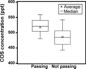
Backward trajectory analysis is a useful for interpreting trace gas variations (e.g., Baartman et al. 2021). The three-day backward trajectories start from the AIST site at 3:00, 9:00, 15:00, and 21:00 JST daily, and the starting height was set at half of the planetary boundary layer using the Hybrid Single-Particle Lagrangian Integrated Trajectory (HYSPLIT) model available online at https://www.arl.noaa.gov/ready/hysplit4.html (Rolph et al. 2017). The meteorological data were obtained from a 1° × 1° grid. The backward trajectories colour-coded based on the COS concentrations are shown in Fig. 15. Air masses arriving at the AIST site during periods of high COS concentrations (> 550 ppt) came from the southwest. Southwest of the AIST site is the Keihin Industrial Zone. Based on observations conducted from February to April 2001, the Pacific Belt, including the Keihin Industrial Zone, was reported to be an area of high COS emissions from carbon black production, aluminium production, pigment production, sulfur recovery, and CS2 emissions from rayon production (Blake et al. 2004). The change in COS emissions from 2001 to the present is unknown and beyond the scope of this study, but the industrial area has not changed in the past 20 years, and COS emissions are likely occurring in the Pacific Belt, including the Keihin Industrial Zone. After released, CS2 is rapidly converted into COS and sulfur dioxide in the atmosphere (Chin and Davis 1995; Li et al. 2024). Considering that COS concentrations over 550 ppt were seldom observed at remote sites worldwide by NOAA/ESRL and that the air masses always come from the southwest, the increased COS concentrations are likely attributed to anthropogenic emissions from areas such as the Keihin Industrial Zone. We also plotted the COS concentration in box plots, distinguishing air masses passing/not passing through the Keihin Industrial Zone (Fig. 16). The average concentration of air masses passing and not passing the Keihin Industrial Zone was 518 ± 32 ppt and 486 ± 29 ppt, respectively. A t-test was performed on the air masses passing/not passing the Keihin Industrial Zone, revealing significantly different in COS concentrations. This indicates that the Keihin Industrial Zone could be a potential source of the COS. Estimating the source flux of COS from a single point observation over a short period is challenging; however, building a network of low-power continuous measurement systems can help to identify the source of COS.

5. Conclusions
We designed the continuous measurement system from the portable laser-based analyser to measure ambient COS concentration. This system consumes less power than previously reported COS analysers. To achieve precise COS concentration measurements, the change of temperature of the optical cell was within 0.13 ± 0.014 °C h−1 using double insulation with refrigerators and insulation material. A reference gas was introduced for 30 s every min (1 cycle min−1) to cancel temporal drifts of the measured COS concentrations. The difference between the H2Oref and H2Osam was within ± 400 ppm using a parallel flow Nafion dryer to reduce the effect of the difference between the H2Oref and H2Osam on the COS concentration. Furthermore, ambient air with COS reduced air using activated charcoal can be used as a reference gas and analysed at regular intervals. The COS concentration was determined using three calibrations gases with a wide COS concentration range (360–565 ppt) purchased from NOAA. A 15-min averaging precision (1σ) for COS concentrations was 12.1 ppt. The continuous measurement system consumes 150 W less power than previously reported COS analysers, and its compactness makes it suitable for field measurements.
We observed the COS concentrations in Tsukuba, Japan, using the designed system for 10 days in April 2023. The observed COS concentrations ranged from 410 ppt to 599 ppt, with an average and a standard deviation (1σ) of 494 ± 33 ppt. The observed values were consistent with previous observations and exhibited diurnal variations. According to the backward trajectory analysis, air masses with high COS concentrations above 550 ppt came from the southwest and passed over the Keihin Industrial Zone in Japan, where anthropogenic COS emissions are high. The continuous measurement system can be used to observe actual atmospheric COS concentration variations and anthropogenic fluxes. The system is designed to detect diurnal variations in COS concentration. However, additionally temperature control, preparation of several secondary calibration gases, and individual adjustment of switching times between sample and reference gases could be useful, depending on the objective of the observation.
Supplements
Supplement 1: COS concentrations differences with or without the Teflon-coated pump and ECU.
Acknowledgments
We would like to thank Shohei Hattori at the Tokyo Institute of Technology, Japan (current address: International Center for Isotope Effects Research Nanjing University, China) for informing us about the MIRA Pico. The Tateno weather station data were provided by the Japan Meteorological Agency (https://www.jma.go.jp/jma/indexe.html). We also acknowledge the use of the HYSPLIT transport and dispersion model of the Air Resources Laboratory (ARL), which is available online at http://www.arl.noaa.gov/ready.html. This study was supported by Grants-in-Aid for Scientific Research 20J01445 (K.K), 22K18028 (K.K.), 20H01975 (S.O.D. and K.K.), 22H03739 (K.K. and S.I.), 22H00564 (K.K. and S.I.), and 22H05006 (S.I.) from the Ministry of Education, Culture, Sports, Science, and Technology (MEXT), Japan and by Joint Usage/Research Grant of the River Basin Research Center (2021–2022), Gifu University. We would like to thank the reviewers for their valuable comments and suggestions.
References
- Allan, D. W., 1987: Time and frequency (time-domain) characterization, estimation, and prediction of precision clocks and oscillators. IEEE Trans. Ultrason. Ferroelectrics, and Frequency Control., 34, 647–654.
- Baartman, S. L., M. C. Krol, T. Röckmann, S. Hattori, K. Kamezaki, N. Yoshida, and M. E. Popa, 2021: A GC-IRMS method for measuring sulfur isotope ratios of carbonyl sulfide from small air samples. Open Res. Eur., 1, 105, doi: 10.12688/openreseurope.13875.2.
- Bahlmann, E., I. Weinberg, R. Seifert, C. Tubbesing, and W. Michaelis, 2011: A high volume sampling system for isotope determination of volatile halocarbons and hydrocarbons. Atmos. Meas. Tech., 4, 2073–2086.
- Berchet, A., I. Pison, C. Huselstein, C. Narbaud, M. Remaud, S. Belviso, C. Abadie, and F. Maignan, 2024: Can we gain knowledge on COS anthropogenic and biogenic emissions from a single atmospheric mixing ratios measurement site? EGUsphere [preprint], doi: 10.5194/egusphere-2024-549.
- Belviso, S., I. M. Reiter, B. Loubet, V. Gros, J. Lathière, D. Montagne, M. Delmotte, M. Ramonet, C. Kalogridis, B. Lebegue, N. Bonnaire, V. Kazan, T. Gauquelin, C. Fernandez, and B. Genty, 2016: A top-down approach of surface carbonyl sulfide exchange by a Mediterranean oak forest ecosystem in southern France. Atmos. Chem. Phys., 16, 14909–14923.
- Belviso, S., B. Lebegue, M. Ramonet, V. Kazan, I. Pison, A. Berchet, M. Delmotte, C. Yver-Kwok, D. Montagne, and P. Ciais, 2020: A top-down approach of sources and non-photosynthetic sinks of carbonyl sulfide from atmospheric measurements over multiple years in the Paris region (France). PLoS One, 15, e0228419, doi: 10.1371/journal.pone.0228419.
- Berkelhammer, M., D. Asaf, C. Still, S. Montzka, D. Noone, M. Gupta, R. Provencal, H. Chen, and D. Yakir, 2014: Constraining surface carbon fluxes using in situ measurements of carbonyl sulfide and carbon dioxide. Global Biogeochem. Cycles, 28, 161–179.
- Berkelhammer, M., H. C. Steen-Larsen, A. Cosgrove, A. J. Peters, R. Johnson, M. Hayden, and S. A. Montzka, 2016: Radiation and atmospheric circulation controls on carbonyl sulfide concentrations in the marine boundary layer. J. Geophys. Res.: Atmos., 121, 13113–13128.
- Berry, J., A. Wolf, J. E. Campbell, I. Baker, N. Blake, D. Blake, A. S. Denning, S. R. Kawa, S. A. Montzka, U. Seibt, K. Stimler, D. Yakir, and Z. Zhu, 2013: A coupled model of the global cycles of carbonyl sulfide and CO2: A possible new window on the carbon cycle. J. Geophys. Res.: Biogeosci., 118, 842–852.
- Blake, N. J., D. G. Streets, J.-H. Woo, I. J. Simpson, J. Green, S. Meinardi, K. Kita, E. Atlas, H. E. Fuelberg, G. Sachse, M. A. Avery, S. A. Vay, R. W. Talbot, J. E. Dibb, A. R. Bandy, D. C. Thornton, F. S. Rowland, and D. R. Blake, 2004: Carbonyl sulfide and carbon disulfide: Large-scale distributions over the western Pacific and emissions from Asia during TRACE-P. J. Geophys. Res., 109, D15S05, doi: 10.1029/2003JD004259.
- Campbell, J. E., G. R. Carmichael, T. Chai, M. Mena-Carrasco, Y. Tang, D. R. Blake, N. J. Blake, S. A. Vay, G. J. Collatz, I. Baker, J. A. Berry, S. A. Montzka, C. Sweeney, J. L. Schnoor, and C. O. Stanier, 2008: Photosynthetic control of atmospheric carbonyl sulfide during the growing season. Science, 322, 1085–1088.
- Campbell, J. E., M. E. Whelan, U. Seibt, S. J. Smith, J. A. Berry, and T. W. Hilton, 2015: Atmospheric carbonyl sulfide sources from anthropogenic activity: Implications for carbon cycle constraints. Geophys. Res. Lett., 42, 3004–3010.
- Campbell, J. E., M. E. Whelan, J. A. Berry, T. W. Hilton, A. Zumkehr, J. Stinecipher, Y. Lu, A. Kornfeld, U. Seibt, T. E. Dawson, S. A. Montzka, I. T. Baker, S. Kulkarni, Y. Wang, S. C. Herndon, M. S. Zahniser, R. Commane, and M. E. Loik, 2017: Plant uptake of atmospheric carbonyl sulfide in coast redwood forests. J. Geophys. Res.: Biogeosci., 122, 3391–3404.
- Cao, Q., K.-C. Xie, Y. K. Lv, and W. R. Bao, 2006: Process effects on activated carbon with large specific surface area from corn cob. Bioresour. Technol., 97, 110–115.
- Chin, M., and D. D. Davis, 1995: A reanalysis of carbonyl sulfide as a source of stratospheric background sulfur aerosol. J. Geophys. Res., 100, 8993–9005.
- Commane, R., S. C. Herndon, M. S. Zahniser, B. M. Lerner, J. B. McManus, J. W. Munger, D. D. Nelson, and S. C. Wofsy, 2013: Carbonyl sulfide in the planetary boundary layer: Coastal and continental influences. J. Geophys. Res.: Atmos., 118, 8001–8009.
- Crutzen, P. J., 1976: The possible importance of CSO for the sulfate layer of the stratosphere. Geophys. Res. Lett., 3, 73–76.
- Glatthor, N., M. Höpfner, A. Leyser, G. P. Stiller, T. von Clarmann, U. Grabowski, S. Kellmann, A. Linden, B.-M. Sinnhuber, G. Krysztofiak, and K. A. Walker, 2017: Global carbonyl sulfide (OCS) measured by MIPAS/Envisat during 2002–2012. Atmos. Chem. Phys., 17, 2631–2652.
- Hazan, L., J. Tarniewicz, M. Ramonet, O. Laurent, and A. Abbaris, 2016: Automatic processing of atmospheric CO2 and CH4 mole fractions at the ICOS Atmosphere Thematic Centre. Atmos. Meas. Tech., 9, 4719–4736.
- Hattori, S., K. Kamezaki, and N. Yoshida, 2020: Constraining the atmospheric OCS budget from sulfur isotopes. Proc. Natl. Acad. Sci. U. S. A., 117, 20447–20452.
- Kato, H., M. Saito, Y. Nagahata, and Y. Katayama, 2008: Degradation of ambient carbonyl sulfide by Mycobacterium spp. in soil. Microbiology, 154, 249–255.
- Kamezaki, K., S. Hattori, T. Ogawa, S. Toyoda, H. Kato, Y. Katayama, and N. Yoshida, 2016: Sulfur isotopic fractionation of carbonyl sulfide during degradation by soil bacteria. Environ. Sci. Technol., 50, 3537–3544.
- Kamezaki, K., S. Hattori, E. Bahlmann, and N. Yoshida, 2019: Large-volume air sample system for measuring 34S/32S isotope ratio of carbonyl sulfide. Atmos. Meas. Tech., 12, 1141–1154.
- Kettle, A. J., U. Kuhn, M. von Hobe, J. Kesselmeier, and M. O. Andreae, 2002: Global budget of atmospheric carbonyl sulfide: Temporal and spatial variations of the dominant sources and sinks. J. Geophys. Res., 107, ACH 25-1–ACH 25-16.
- Kooijmans, L. M. J., N. A. M. Uitslag, M. S. Zahniser, D. D. Nelson, S. A. Montzka, and H. Chen, 2016: Continuous and high-precision atmospheric concentration measurements of COS, CO2, CO and H2O using a quantum cascade laser spectrometer (QCLS). Atmos. Meas. Tech., 9, 5293–5314.
- Kuai, L., J. R. Worden, J. E. Campbell, S. S. Kulawik, K.-F. Li, M. Lee, R. J. Weidner, S. A. Montzka, F. L. Moore, J. A. Berry, I. Baker, A. Scott Denning, H. Bian, K. W. Bowman, J. Liu, and Y. L. Yung, 2015: Estimate of carbonyl sulfide tropical oceanic surface fluxes using Aura Tropospheric Emission Spectrometer observations. J. Geophys. Res.: Atmos., 120, 11012–11023.
- Li, Y., K. Kamezaki, and S. O. Danielache, 2024: Photooxidation pathway as a potential CS2 sink in the atmosphere. Geochem. J., 58, 169–183.
- Ma, J., M. Remaud, P. Peylin, P. Patra, Y. Niwa, C. Rodenbeck, M. Cartwright, J. J. Harrison, M. P. Chipperfield, R. J. Pope, C. Wilson, S. Belviso, S. A. Montzka, I. Vimont, F. Moore, E. L. Atlas, E. Schwartz, and M. C. Krol, 2023: Intercomparison of atmospheric carbonyl sulfide (TransCom-COS): 2. Evaluation of optimized fluxes using ground-based and aircraft observations. J. Geophys. Res.: Atmos., 128, e2023JD039198, doi: 10.1029/2023JD039198.
- Montzka, S. A., M. Aydin, M. Battle, J. H. Butler, E. S. Saltzman, B. D. Hall, A. D. Clarke, D. Mondeel, and J. W. Elkins, 2004: A 350-year atmospheric history for carbonyl sulfide inferred from Antarctic firn air and air trapped in ice. J. Geophys. Res., 109, D22302, doi: 10.1029/2004JD004686.
- Montzka, S. A., P. Calvert, B. D. Hall, J. W. Elkins, T. J. Conway, P. P. Tans, and C. Sweeney, 2007: On the global distribution, seasonality, and budget of atmospheric carbonyl sulfide (COS) and some similarities to CO2. J. Geophys. Res., 112, D09302, doi: 10.1029/2006JD007665.
- Mouat, A. P., Z. A. Siegel, and J. Kaiser, 2024: Evaluation of Aeris mid-infrared absorption (MIRA), Picarro CRDS (cavity ring-down spectroscopy) G2307, and dinitrophenylhydrazine (DNPH)-based sampling for long-term formaldehyde monitoring efforts. Atmos. Meas. Tech., 17, 1979–1994.
- Rastogi, B., M. Berkelhammer, S. Wharton, M. E. Whelan, F. C. Meinzer, D. Noone, and C. J. Still, 2018: Ecosystem fluxes of carbonyl sulfide in an old-growth forest: Temporal dynamics and responses to diffuse radiation and heat waves. Biogeosciences, 15, 7127–7139.
- Rolph, G., A. Stein, and B. Stunder, 2017: Real-time environmental applications and display system: READY. Environ. Modell. Software, 95, 210–228.
- Stimler, K., D. Nelson, and D. Yakir, 2010a: High precision measurements of atmospheric concentrations and plant exchange rates of carbonyl sulfide using mid-IR quantum cascade laser. Global Change Biol., 16, 2496–2503.
- Stimler, K., S. A. Montzka, J. A. Berry, Y. Rudich, and D. Yakir, 2010b: Relationships between carbonyl sulfide (COS) and CO2 during leaf gas exchange. New Phytol., 186, 869–878.
- Von Hobe, M., D. Taraborrelli, S. Alber, B. Bohn, H.-P. Dorn, H. Fuchs, Y. Li, C. Qiu, F. Rohrer, R. Sommariva, F. Stroh, Z. Tan, S. Wedel, and A. Novelli, 2023: Measurement report: Carbonyl sulfide production during dimethyl sulfide oxidation in the atmospheric simulation chamber SAPHIR. Atmos. Chem. Phys., 23, 10609–10623.
- Whelan, M. E., S. T. Lennartz, T. E. Gimeno, R. Wehr, G. Wohlfahrt, Y. Wang, L. M. J. Kooijmans, T. W. Hilton, S. Belviso, P. Peylin, R. Commane, W. Sun, H. Chen, L. Kuai, I. Mammarella, K. Maseyk, M. Berkelhammer, K.-F. Li, D. Yakir, A. Zumkehr, Y. Katayama, J. Ogée, F. M. Spielmann, F. Kitz, B. Rastogi, J. Kesselmeier, J. Marshall, K.-M. Erkkilä, L. Wingate, L. K. Meredith, W. He, R. Bunk, T. Launois, T. Vesala, J. A. Schmidt, C. G. Fichot, U. Seibt, S. Saleska, E. S. Saltzman, S. A. Montzka, J. A. Berry, and J. E. Campbell, 2018: Reviews and syntheses: Carbonyl sulfide as a multi-scale tracer for carbon and water cycles. Biogeosciences, 15, 3625–3657.
- Zanchetta, A., L. M. J. Kooijmans, S. van Heuven, A. Scifo, H. Scheeren, I. Mammarella, U. Karstens, J. Ma, M. Krol, and H. Chen, 2023: Sources and sinks of carbonyl sulfide inferred from tower and mobile atmospheric observations. Biogeosciences, 20, 3539–3553.
- Zumkehr, A., T. W. Hilton, M. Whelan, S. Smith, L. Kuai, J. Worden, and J. E. Campbell, 2018: Global gridded anthropogenic emissions inventory of carbonyl sulfide. Atmos. Environ., 183, 11–19.