Abstract
Linear eigenvalue analysis of the primitive equations is performed to study atmospheric free oscillations under the influence of a zonal mean field. The model for the primitive equations is based on a three-dimensional spectral formulation, and the zonal mean field is produced by averaging reanalysis data over 10 years. The frequencies and latitudinal/vertical structures of the eigenmodes obtained by the analysis are compared with the results of the classical tidal theory and with those of the free oscillation modes detected from reanalysis data by a recent study. The frequencies and vertical structures of the eigenmodes obtained in the present study are consistent with those of the eigenmodes detected in the recent study, while the obtained latitudinal structures do not differ significantly from those of the classical tidal theory. It is shown that the deviation from the frequency obtained from the classical tidal theory is mainly due to the effect of the zonal mean flow, but partly also to the latitudinal variation of the temperature field. The present study also shows that the vertical phase structure of the obtained eigenmodes, which is inconsistent with the classical tidal theory, can be understood qualitatively by using the wave dispersion relation.
1. Introduction
The study of the free oscillations of the Earth’s atmosphere has long been developed in a common framework with the study of atmospheric tides. The free oscillations are solutions of normal modes without forcing satisfying the rigid boundary condition at the bottom and the energy decay boundary condition at the top. When the primitive equations are linearized from a stationary atmosphere as the reference field, the system is separated into the horizontal structure equation, or Laplace’s tidal equation (LTE), and the vertical structure equation (VSE) if the temperature is a function of altitude only. The vertical structure of the normal mode solution has the same structure as that of the Lamb wave (Lamb 1911) if the atmosphere is isothermal, and the corresponding equivalent depth h is given as h = γH, where γ is the heat capacity ratio and H is the scale height of the isothermal atmosphere, and the latitudinal structure is determined by solving the LTE for the equivalent depth. For these details, including the historical background, see Chapman and Lindzen (1970).
The Earth’s atmosphere is, of course, neither isothermal nor stationary, but Taylor (1929) estimated the equivalent depth to be about 10.4 km based on the propagation speed of pressure disturbances observed during the 1883 eruption of Krakatoa. Since then, the equivalent depth of the free oscillations of the Earth’s atmosphere has been considered to be about 10 km, and this has also been considered to be the only equivalent depth for the realistic vertical temperature profile of the Earth’s atmosphere (However, there have recently been new studies on this subject, which will be discussed later in this section).
Once the equivalent depth is determined, the eigenfrequencies and latitudinal structures of the normal modes can be determined by (numerically) solving the LTE according to the method of Longuet-Higgins (1968). Many studies have been carried out to detect the free oscillation modes of the atmosphere determined in this way from observational data. For example, the global Rossby modes were detected from satellite observations of the upper stratosphere by Hirota and Hirooka (1984). However, these studies were limited to relatively long period modes, and the detection of short period free oscillation modes had to wait for Sakazaki and Hamilton (2020) (for a detailed review of the history of attempts to detect free oscillation modes, see the description therein).
In Sakazaki and Hamilton (2020), it was shown that free oscillation modes with periods not only of several days but also of as short as about 2 hours could be comprehensively detected by spectral analysis of 38 years of hourly global reanalysis data, although not the observational data, and there the frequency, vertical structure, and latitudinal structure of the detected modes were compared with those of the LTE solutions for a stationary atmosphere. As a result, it was shown that the frequency of the detected modes was most consistent with that of the LTE solution when the equivalent depth was set to 10 km, but there were some differences from the classical tidal theory in the frequency and latitudinal/vertical structure, reflecting the fact that the real atmosphere has a non-zero zonal wind field and a latitudinally dependent temperature field, and that the bottom boundary is not horizontally uniform.
How the normal modes of free oscillations vary with the background field was studied by Geisler and Dickinson (1976), Schoeberl and Clark (1980), and Salby (1981a, b). In particular, in Salby (1981a, b), realistic latitudinal/vertical structures of zonally uniform zonal wind and temperature fields were given and a periodic external forcing was applied to the linearized primitive equations with respect to the given basic field to extract modes showing amplitude increase near resonance. He showed that the frequencies of the Rossby and Rossby-gravity modes were consistent with those of the modes detected in the observational studies. However, since the method used there was to study the response to periodic forcings to the linearized equations, the individual eigenmodes were not considered to be completely separated, and the modes considered there were also limited to those with relatively long periods. On the other hand, Kasahara (1980) performed a linear eigenvalue analysis using a linearized shallow water equation by setting the zonal flow profile at the 500 hPa surface and the balanced height field to it as the basic field. There, the eigenmodes were obtained comprehensively, including not only Rossby and Rossby-gravity modes but also Kelvin and gravity modes. The eigenfrequencies and latitudinal structures of the modes were studied in relation to the LTE solution, to clarify how they vary with the zonal flow profile (and the height field balanced by the zonal flow). However, this calculation was performed only for a barotropic atmosphere, and it was not possible to investigate how the baroclinicity of the zonal flow affects the normal modes.
Based on the above research background, in the present study, we extend the research of Kasahara (1980) to a baroclinic atmosphere by performing a direct eigenvalue analysis of the three-dimensional primitive equations linearized with respect to a basic field in which the latitudinal/vertical structures of a realistic zonally uniform zonal wind field and temperature field are specified. We investigate how the frequencies and latitudinal/vertical structures of the normal mode solutions are affected by the background field. By performing a direct eigenvalue analysis, all types of Lamb modes are treated comprehensively and compared with the modes detected by Sakazaki and Hamilton (2020) in order to clarify to what extent the effect of the background field can explain the difference in characteristics between the modes detected by Sakazaki and Hamilton (2020) and the normal mode solutions for a stationary atmosphere. In the present study, modes with vertical structures corresponding to Lamb waves are referred to as Lamb modes, including when they are deformed by the background field.
Before closing this section, the possible existence of free oscillation modes with equivalent depths smaller than about 10 km should also be mentioned. As mentioned above, the equivalent depth has only one value in the case of an isothermal atmosphere, but the temperature of the real atmosphere varies significantly in the vertical direction. Depending on the vertical profile of the temperature, there may be several equivalent depths for which there exist solutions satisfying the lower and upper boundary conditions for the VSE. In fact, Pekeris (1937) showed that, by assuming unrealistically high temperatures for the stratopause, an equivalent depth mode of about 8 km could exist, in addition to about 10 km. However, in Salby (1979), using a more realistic temperature profile, U.S. Standard Atmosphere, 1976, the equivalent depths obtained (although the mode was not completely evanescent at the top, since the very high temperature thermosphere was also taken into account there) were shown to be 9.6 km and 5.8 km. The latter corresponds to the mode predicted by Pekeris (1937), the reality of which was first demonstrated in Watanabe et al. (2022), which first detected the predicted mode from an analysis of satellite brightness temperature data during the 2022 eruption of the Hunga Tonga-Hunga Ha’apai volcano. There, not only the Lamb wave propagating at a phase velocity corresponding to about 10.1 km equivalent depth was detected, but also a wave packet propagating at a phase velocity corresponding to about 6.1 km equivalent depth, and the latter was named the Pekeris wave in Watanabe et al. (2022). This equivalent depth of 6.1 km differs from the 5.8 km obtained by Salby (1979), but Ishioka (2023) pointed out a problem with the accuracy of the calculation in Salby (1979) and showed that the corresponding equivalent depth was 6.6 km when calculated correctly using the temperature profile of U.S. Standard Atmosphere, 1976. Furthermore, Ishizaki et al. (2023) showed that the equivalent depth of the Pekeris wave was about 6.5 km, even using the vertical profile of the average temperature in the tropics at the time of the 2022 eruption of the Hunga Tonga-Hunga Ha’apai volcano, which corresponds better to the position of the spectral peak of the Kelvin wave in the spectral analysis of the reanalysis data in Watanabe et al. (2022). The term atmospheric free oscillation usually refers to Lamb modes, but considering the recent studies mentioned above, those with vertical structures corresponding to the Pekeris wave should also be considered and are referred to as Pekeris modes. However, in the present study, we do not consider Pekeris modes not only because we intend to focus mainly on the comparison with the Sakazaki and Hamilton (2020) results, but also because in order to properly extract Pekeris modes as eigenmodes, more vertical expansion degrees of freedom are required, as described in the next section, which makes the numerical calculations more difficult.
The remainder of the present study is organized as follows. In Section 2, we describe the method of the eigenvalue analysis of free oscillation including the effect of a zonal mean field which is determined by averaging reanalysis data. The results of the eigenvalue analysis are presented in Section 3. Discussion is presented in Section 4, along with additional analyses to interpret the results of the eigenvalue analysis. Summary is given in Section 5.
2. Methods and data
In the present study, we perform a linear eigenvalueeigenvector analysis for the case of a perturbation applied to a zonally uniform field, using a system of primitive equations in σ-coordinates on a rotating sphere as the governing equations. We follow the formulation of Ishioka et al. (2022) and use the completely non-dimensionalized primitive equations, where the length scale, the temperature scale, and the time scale are nondimensionalized by using the radius of the sphere (a*), the reference temperature (T0*), and  , respectively. Here, R* is the gas constant for the dry atmosphere. The full nonlinear primitive equations are omitted here (see Ishioka et al. 2022) because it would be redundant, but the linearized equations, given an infinitesimally small perturbation to a zonally uniform basic field, can be written as follows.
Here, Ω is angular velocity of the sphere, κ = R*/Cp*, where Cp* is specific heat at constant pressure, t is time, λ is longitude, μ = sin ϕ, where ϕ is latitude, σ = p*/p0* , where p* is pressure and p0* is surface pressure of the basic state. Note that since the effect of the μ dependence of p0* is considered to be small, as shown by Ishizaki et al. (2023) in calculating the equivalent depths of the Lamb and Pekeris modes, we assume here for simplicity that p0* is uniform in the μ direction. The temperature field and the eastward wind field of the basic state are represented by T(μ, σ) and U(μ, σ), respectively. The variable  is defined as
  , where
  is the surface pressure perturbation,
  is the geopotential perturbation,
  is the temperature perturbation, and the variables
  and
and  are the perturbations of the horizontal divergence and the vertical component of the vorticity, respectively. The rightmost terms
  in (1)–(3) are dissipation terms which will be defined later. The variable
  is the velocity potential perturbation, and ψ̃ is the stream function perturbation. Note that the above parameters and variables without the subscript “*” are inherently dimensionless, or have been nondimensionalized as described above.
As a preparation for deriving the eigenvalue calculation form of a matrix, we assume the following wave-like solution for the longitude-time dependence of the field of each perturbation,
Here, Re(∙) means to take real parts and  . Note that the reason why the imaginary unit is attached differently depending on the type of perturbation is to ensure that the final matrix for the eigenvalue calculation is a real matrix (when dissipative effects are not considered). Substituting the expression (15)–(30) into (1)–(14), we obtain the following equations.
Next, we expand  , , , and
  in the μ direction by the associated Legendre functions and in the σ direction by the Legendre polynomials as follows.
Here, Pn,m(μ) is the associated Legendre function, which is defined as follows,
and the parameters M and L are the horizontal and vertical truncation wavenumber, respectively. The Legendre polynomial Pl(1-2σ) is defined as the case where n = l and m = 0 with μ = 1 - 2σ. Note that in (47) the right-hand side is multiplied by σ to eliminate the singularity of the function under integration on the right-hand side of (39) and that since does not depend on σ, so there is no expansion in the σ direction for (48).
Formally substituting (45)–(48) into (31)–(34) and multiplying both sides of (45) and (46) by Pn,m(μ) Pl(1 - 2σ), both sides of (47) by σPn, m(μ) Pl(1 - 2σ) and both sides of (48) by Pn,m(μ) and integrating both sides of (45)–(48) in the interval [-1, 1] for μ and in the interval [0, 1] for σ (i.e., applying the Galerkin method), we obtain a matrix eigenvalue problem for each zonal wavenumber m of the following form after several matrix operations (for details see Ishioka et al. 2022).
Here, v is an N-dimensional vector, where N = 3(M - m + 1)(L + 1), consisting of (ζm,0, … , ζM,L, δm,0, … , δM,L, τm,0, … , τM,L-1 , sm, … , sM ), and A is an N × N matrix. This is a problem of finding the eigenvalues and eigenvectors of the matrix, where the real part of ω is the eigenfrequency of the eigenmode and the imaginary part of ω is the growth rate of the eigenmode (if the imaginary part is negative, its absolute value is the decay rate).
Note that the integration in [-1, 1] with respect to μ and the integration in [0, 1] with respect to σ required to derive (50) are done by multiplying the values in the Gaussian node by the Gaussian weight and summing, unless it is easy to do the integration analytically. That is, if F(μ) and G(σ) are the integration functions depending on μ and σ respectively, the numerical integration is performed as follows.
Here, ( μj, wj) (j = 1, 2, … , J) and (σk, Wk) (k = 1, 2, … , K) are the (Gaussian nodes, Gaussian weights) for μ and σ spaces, respectively. For their definitions when setting the numbers of the Gaussian nodes J and K, please see Ishioka et al. (2022). In addition, in the derivation of (50), we need to mention how to treat the basic fields U(μ, σ) and T(μ, σ) and their partial derivatives. As we will see later, U and T are given by the grid values of reanalysis data, but the positions of the grid points in the μ and σ directions are different from those of the Gaussian nodes above. First, for the μ direction, noting that μ = sin ϕ and using the given grid point data, we perform a discrete sine series expansion for U by the colatitude π/2 - ϕ and a discrete cosine series expansion for T, and then use the expansion to obtain their values and their μ partial derivatives at the Gaussian node μj(j = 1, 2, …, J) by interpolation. For the σ direction, the dimensionless logarithmic pressure coordinate z = -ln σ is introduced and the grid data are linearly interpolated to the values at zk = -ln σk(k = 1, 2, … , K) corresponding to the Gaussian nodes in the z coordinate. The σ partial differential values are calculated from the z partial differential values in the linearly interpolated interval.
The basic framework of the eigenvalue analysis method in the present study has been described above, but in order to extract the deformed Lamb modes as eigenmodes given a realistic basic field, several additional procedures are required, as described below. First of all, even in the implementation of the 3D spectral method for the primitive equations that we are now using, the domain that extends infinitely in the vertical direction is calculated in the finite domain [0, 1] of σ . In the present study, as can be seen from (8), the boundary condition of  is imposed at the σ = 0 surface, so energy cannot escape upwards. Due to the reflection of waves from such an upper boundary, when eigenvalue analysis is performed without dissipative terms, many spurious modes (which cannot naturally exist) will appear as eigenmodes satisfying the boundary conditions (e.g., Lindzen et al. 1968). Therefore, it is necessary to set up a region that acts as a sponge to suppress the effect of reflection from the upper boundary and to increase the damping rate of such spurious modes so that the Lamb modes, which are the natural free oscillation modes, can be separated from them. With this intention, the dissipation terms
  are introduced as the following equations in the form of Rayleigh friction or Newtonian cooling:
Here, we consider the following form as the σ dependence of α.
where αR and σR are the parameters that determine the strength of the dissipation and the σ range in which it acts, respectively. The function form of this α is such that α → αR(σ → 0), but if σR ≪ 1 then α ≪ αR as σ → 1. In other words, the upper atmosphere that satisfies σ < σR has a sponge-like effect, while the dissipation becomes almost ineffective in the lower atmosphere where the energy of the Lamb mode is large. In the present study, we set σR = 1 × 10⁻³ and  , where αR* = 1 × 10⁻⁵ s−1, not only to suppress the spurious modes sufficiently but also to keep the eigenfrequencies and the latitudinal/vertical structures of the eigenmodes to be as unaffected as possible by the dissipation. Figure 1 shows the vertical profile of the relaxation time due to dissipation. The relaxation time is almost one day above 1 hPa, where the dissipative effect is strong, but it increases rapidly with decreasing altitude, reaching about 100 days at 10 hPa and increasing further at lower altitudes, where the dissipative effect becomes negligible. Thus, the vertical structures of the eigenmodes obtained in the next section are affected by dissipation above about 10 hPa and should be treated with caution. The effect of this dissipation parameter on the eigenfrequencies and the structure of the eigenmodes is discussed at the beginning of the next section.

Fig. 1. The vertical profile of dissipation relaxation times introduced into the eigenvalue analysis model.
Even with the sponge layer set up as described above, the damping rates of spurious eigenmodes with vertical nodes are not sufficiently large, and it is difficult to objectively distinguish them from Lamb modes deformed in the basic field only by the amplitude of the damping rate. Therefore, we consider the orthogonal relationship between the eigenmodes and the vertical phase structure to separate the modes. First, it is known that the latitudinal structure of the free oscillation modes for a stationary and horizontally isothermal atmosphere has the following orthogonal relationship for each zonal wavenumber m (Kasahara 1976).
Here, the superscript dagger denotes the complex conjugate and the subscript denotes the eigenmode number, and ε is the Lamb parameter, which is defined as,
where, Ω* is the (dimensional) angular velocity of the sphere, g* is the (dimensional) gravity acceleration, and h* is the (dimensional) equivalent depth of the free eigenmode. Also,  represents the zonal wavenumber m component of the (non-dimensionalized) geopotential perturbation in the p coordinate system, and is obtained from
  in the σ coordinate defined by (39) as follows.
where  (σ) is the global mean of T(μ, σ).
Using the formula (54) we can define the inner product taking into account the latitudinal structure of the eigenmodes, but it is inconvenient to use it if the equivalent depth has not been determined beforehand, since the Lamb parameter ε is not determined until the equivalent depth has been determined. As an alternative, we use only the kinetic energy part of (54) and define a function  (σ ) as,
to examine the vertical phase structure of the eigenmodes obtained by solving (50). This (σ ) will be a complex number for which arg [(σ )] can be calculated to examine the global average phase structure of the eigenmode with respect to the σ = 1 surface. If arg [(σ )] = θ, then this eigenmode is phase-shifted to the east by θ at the specified σ surface with respect to the σ = 1 surface. Since the Lamb modes for a stationary and horizontally isothermal atmosphere do not tilt in phase in the vertical direction, the following criteria are imposed in order to extract the Lamb modes deformed by the fundamental field separately from the spurious eigenmodes.
-
A1 |arg[(σ)]| < π/2 at any levels of σ.
-
A2 Select those with eigenfrequencies greater than 1/2 cpd.
Here, cpd is “cycle per day,” and the criterion A2 is imposed to remove the slow “continuous” mode caused by advection by zonal wind. The value 1/2 cpd is introduced by considering that the maximum period of the Kelvin mode is 33 hours. In the present study, when simply referring to the eigenfrequency, we will refer to the absolute value of the eigenfrequency. When it is necessary to refer to the sign, it will be indicated by stating whether the corresponding eigenmode is eastward or westward.
With the A1 and A2 criteria set above, the high frequency Lamb modes can be extracted. However, for the low frequency Lamb modes, that is, the Rossby modes and the westward Rossby-gravity modes, the criterion A2 should obviously not be imposed. Furthermore, for the low frequency modes with large zonal wavenumbers, when given a realistic background field, the westward tilt of the phase of these modes in the upper layer becomes large, and the A1 criterion becomes too strict to extract these modes. We therefore relax the criterion A1 a little and consider allowing a phase tilt in the upper atmosphere as |arg[(σ )]| < π/2 (σ > 0.1). However, when the criterion is relaxed in such a way, spurious modes whose latitudinal structure is far from the Rossby mode and the westward Rossby-gravity mode are also extracted. In order to extract the eigenmodes whose latitudinal structure is consistent with the Rossby mode and the westward Rossby-gravity mode in the stationary atmosphere, we introduce the following inner product and scalar quantities induced by the inner product.
Here, ΘH is the reference solution corresponding to the Rossby or westward Rossby-gravity mode, which is calculated as an eigensolution of the LTE at the equivalent depth of 10 km. On the other hand, ΘM is the surface (at σ = 1) structure of the mode obtained from the eigenvalue analysis to be checked. Note that in (60), the Lamb parameter ε is calculated with h* = 10 km. The scalar value  calculated by (61) takes values in the range [0, 1]. As the value approaches 1, the eigensolution under test ΘM gets closer to the reference solution ΘH . From the above, we introduce the following criteria for extracting the Rossby or westward Rossby-gravity modes.
-
B1 |arg[(σ)]| < π/2 (σ > 0.1).
-
B2 > 0.7.
-
B3 From the modes that satisfy the above two conditions, the one with the lowest damping rate is selected.
Here, the reference solutions used in criterion B2 are only those for the westward Rossby-gravity mode and the 1st Rossby mode with north-south symmetry of the geopotential perturbation field. This is because the extraction of free oscillation modes in the present study is mainly considered for comparison with Sakazaki and Hamilton (2020). In criterion B2, the number 0.7 is somewhat arbitrary, but if this value is too small, modes with latitudinal structures that differ significantly from the latitudinal structure of the mode to be extracted will be mixed in. If the value is too close to 1, the target mode cannot be extracted because the latitudinal structure of the mode is distorted by the zonal mean field. Considering these factors, a figure of 0.7 is adopted, albeit empirically. The criterion of B3 is also imposed because there are cases where the mode is not uniquely determined by the criteria of B1 and B2 alone.
As a background field for the eigenvalue analysis, we use pressure-level (Hersbach et al. 2023) and model-level (Hersbach et al. 2017) zonal wind and temperature data in ERA5 (Hersbach et al. 2020), the latest atmospheric reanalysis dataset produced by the European Centre for Medium-Range Weather Forecasts (ECMWF). The model-level data are used together because, as described in Ishizaki et al. (2023), the ERA5 pressure-level data are only available up to the 1 hPa surface, and the model-level data are used to compensate for the part above that. As described in Ishizaki et al. (2023), model-level data are used at 71.1187 hPa and above, and pressure-level data at 100 hPa and below, which together are used as 81 level data from 1000 hPa to 0.01 hPa. The longitude-latitude grid interval is 1° × 1° for both the model-level data and the pressure-level data. The temporally and zonally averaged background field of the data described above from 2011 to 2020 is used in this analysis. The reason for using 10-year averaged data for the background field in the present study is that Sakazaki and Hamilton (2020) performed a spectral analysis over a whole year and averaged it over 38 years, so it is appropriate to perform an eigenvalue analysis of a climatological field averaged over a long period for comparison with Sakazaki and Hamilton (2020). It should therefore be noted that seasonal dependence is not considered in the present study. The distribution of this field is shown in Fig. 2. In Fig. 2, a strong eastward jet is observed in the tropical mesosphere. This is caused by the model specification as described in Shepherd et al. (2018), but for the Lamb mode, which is the focus of the present study, its energy is trapped near the ground surface and the influence of this unrealistic jet is considered to be negligible, so this background field is used as it is.
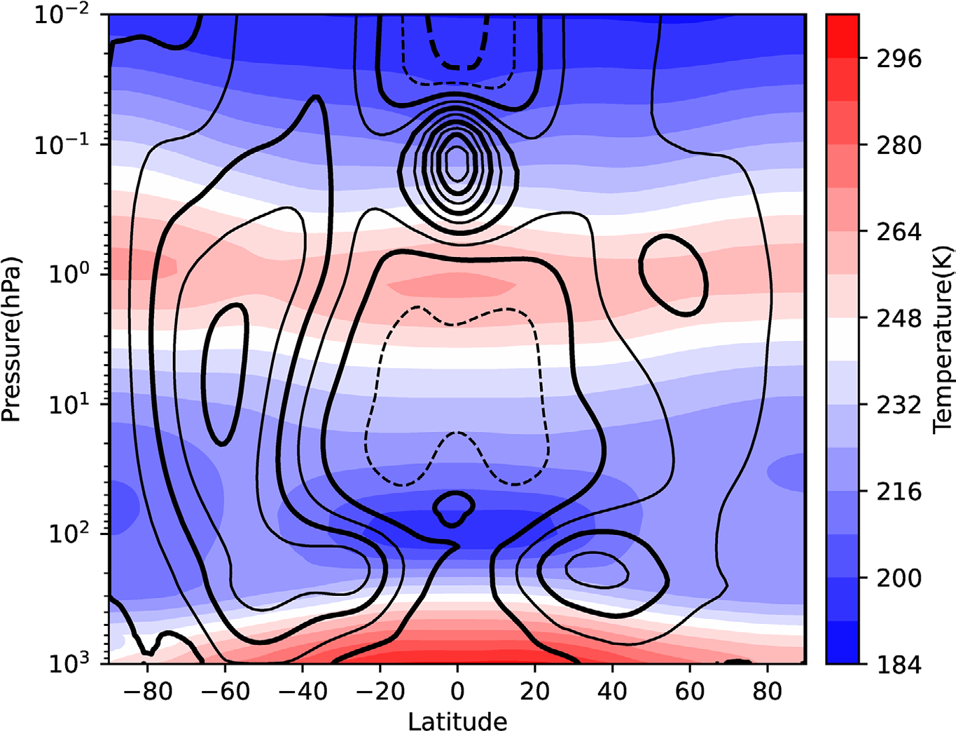
Fig. 2. Distribution of temporally and zonally averaged zonal wind (contours) and temperature (color shading) of the ERA5 monthly averaged data from 2011 to 2020. The contour interval is 8 m s−1 (that of thick line is 16 m s−1) and the dashed
lines show negative values (i.e., westward wind).
The parameters used in the numerical calculations are described below. Ω* = 7.29212 × 10⁻⁵ s−1, R* = 287 m2 s−2 K−1, a* = 6.371229 × 10⁶ m, κ = 2/7, g* = 9.80 m s−2, and p0* = 1000 hPa. The horizontal truncation wavenumber M is 21, the number of latitudinal grid points J = 32. The vertical truncation wavenumber L is set to 85 and the number of vertical grid points K = 128. Then, the top of the vertical grid of the spectral method used for eigenvalue calculations is at 0.0875560 hPa.
3. Results
An eigenvalue analysis is first performed for the linear model used in the present study with a stationary isothermal background field to check the accuracy of the eigenvalue analysis and the effect of the introduced dissipation terms. The isothermal atmospheric temperature T* treated here is determined such that the equivalent depth of the Lamb mode, h* , determined by the following equation, is 10 km.
Here, γ = 1/(1 - κ) = 7/5. Hence, we set T* = 243.90 K. Table 1 shows the dependence of the eigenfrequencies of four representative modes of zonal wavenumber 1 on the two dissipation parameters (σR, αR*). Note that since the phase tilt in the vertical direction is small in the case of a stationary isothermal atmosphere, regardless of the parameters in the dissipation terms, all modes, including the Rossby and westward Rossby-gravity modes can be extracted using only the A1 criterion described in the previous section. In Table 1, as σR or αR* becomes small, the deviation of the eigenfrequency of each eigenmode from the LTE solution decreases and is within 1 % relative error when σR = 1 × 10⁻³ and αR* = 1 × 10⁻⁵ s−1 (the default setting). Therefore, in the default case of dissipation introduced in the present study (D), we have confirmed that the difference from the eigenfrequencies without considering dissipation is small, and we will use this dissipation parameter in the calculations including latitudinal/vertical structures of the zonal wind and temperature field based on the reanalysis data. However, there are cases where the relative error of 1 % can be important, which will be discussed in Section 4.3.

The dependence of the vertical structures of the latitudinally averaged (|ϕ| < 20°) geopotential fields for the corresponding four modes on the dissipation parameters is shown in Fig. 3. Note that for comparison with Sakazaki and Hamilton (2020), the amplitude at each level  (σ) is calculated as follows,
where μ0 = sin 20, and the phase at each level arg [ (σ)] is obtained by taking the argument of the complex number (σ) as follows,
Similar to the eigenfrequency, as σR or αR* becomes small, the deviation of the amplitude and phase profile of each eigenmode from the VSE solution for the stationary isothermal atmosphere decreases, and the deviation does not become significant up to the 10 hPa level when σR = 1 × 10⁻³ and αR* = 1 × 10⁻⁵ s−1 (the default setting). In case (A), where both dissipation parameters are large, the deviation of the amplitude and phase structure from the VSE solution is clearly seen from the level of 100 hPa, but still, in this isothermal stationary atmosphere, the phase tilt is very small compared to the cases of the eigenvalue analysis with the latitudinal/vertical structure of the zonal wind and temperature fields obtained from the reanalysis data, which will be shown later. Nevertheless, referring again to Table 1, it can be seen that in case (A), the eigenfrequency is significantly smaller than that of the LTE solution, which can be interpreted as an effect of the introduction of a sponge layer with a strong dissipative effect in the upper layer of the atmosphere, which effectively reduces the equivalent depth since the dissipative effect limits the vertical extent of the Lamb mode.
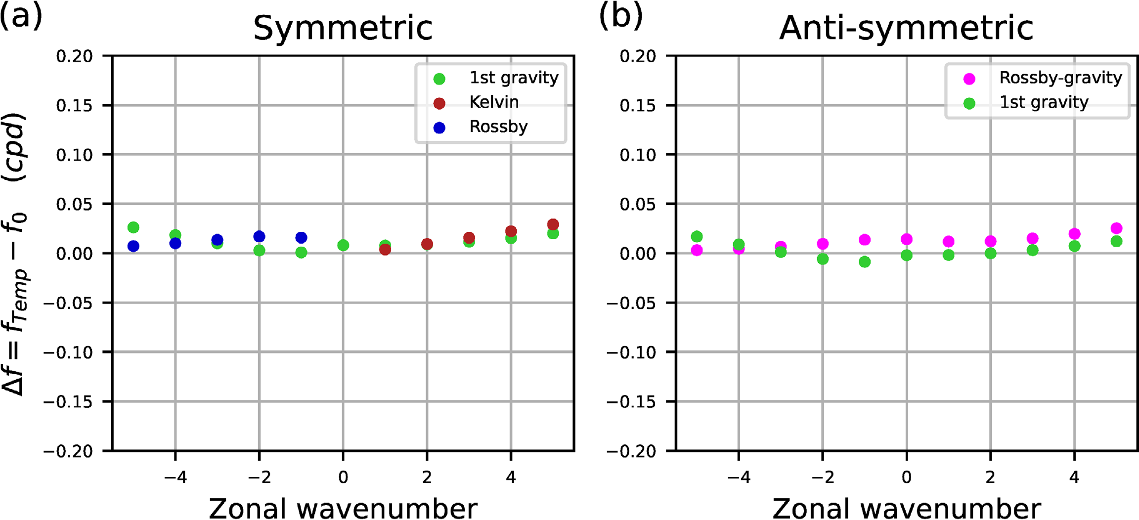
We now consider zonal mean zonal wind and temperature distributions based on the reanalysis data for the eigenvalue analysis. Figure 4 shows the difference between the eigenfrequencies obtained from the eigenvalue analysis for the zonal mean zonal wind and the zonal mean temperature field and those obtained from the LTE with the equivalent depth of 10 km. The reason for showing such deviations is to facilitate comparison with Sakazaki and Hamilton (2020). Except for the Kelvin mode, where the deviation is close to zero, the deviations are positive for the eastward modes and negative for the westward modes, with one exception (Rossby mode with wavenumber 1). The zonal wavenumber dependence of the deviations for each mode obtained from the eigenvalue analysis of the present study is in good quantitative agreement with the results of the spectral analysis of the reanalysis data shown in Figs. 12a and 12b of Sakazaki and Hamilton (2020). As we will see in the next paragraph, this dependence can be understood to some extent as an effect of the Doppler shift due to the zonal flow. However, while the eastward modes, with the exception of the Kelvin modes, show an increase in deviation almost proportional to the zonal wavenumber, the westward modes show a dependence that is not linear, and for the 1st symmetric gravity and Rossby-gravity modes the wavenumber dependence is not even monotonic.

Fig. 4. Deviations (Δf : vertical axis) between the eigenfrequencies obtained from the eigenvalue analysis for the zonal mean zonal wind and the zonal mean temperature field (fModel) and those obtained from the LTE at the equivalent depth of 10 km (fTheory). The horizontal axis is the zonal wavenumber, with positive values indicating eastward modes and negative values westward modes. (a): for equatorially symmetric modes (Kelvin mode, 1st gravity mode, and the gravest Rossby mode). (b): for equatorially antisymmetric modes (Rossby-gravity mode and 1st gravity mode). The color legend is shown in the figure.
Next, in order to clarify the cause of the zonal wavenumber dependence of the deviations shown in Fig. 4, we perform eigenvalue analysis by separately assuming the latitudinal/vertical structure of the zonal mean wind and zonal mean temperature fields based on the reanalysis data. Figure 5 shows the difference between the eigenfrequencies obtained from the eigenvalue analysis for the zonal mean zonal wind but with the global mean temperature field and those obtained from the eigenvalue analysis without the background wind but with the global mean temperature field. Similar to Fig. 4, the deviations are close to zero for Kelvin waves and, with one exception (westward 1st antisymmetric gravity mode with zonal wavenumber 1, the cause of which is discussed in Section 4.1), positive for eastward modes and negative for westward modes, which is considered to be an effect of the Doppler shift caused by mid-latitude westerly winds. The non-linear dependence of the deviation on the zonal wavenumber in the westward mode is also similar, although the value itself is different from the results in Fig. 4. However, there is a noticeable difference between the results shown in Figs. 5 and 4 in that in the former the deviation for the Rossby mode of wavenumber 1 is almost zero, so the positive deviation in the latter is not attributed to the zonal wind effect.

The effect of the latitudinal/vertical structure of the zonal mean temperature field is shown in Fig. 6 without the effect of the zonal mean wind. Compared to Fig. 5, the deviations in Fig. 6 are small overall, indicating that the influence of the latitudinal variation of the temperature field is smaller than that of the zonal wind. From Fig. 6, it is clear that the latitudinal variation of the temperature field has the effect of increasing the eigenfrequencies of the Rossby modes, the cause of which will be discussed in Section 4.2. Therefore, the deviation of the Rossby mode with zonal wavenumber 1 in Fig. 4 is positive because the effect of the latitudinal variation of the temperature field exceeds that of the zonal wind. Note that the deviations shown in Fig. 4 are roughly equal to the sum of those in Fig. 5 and those in Fig. 6 for the Rossby and westward Rossby-gravity modes, but not for the other modes. The reason for this is discussed in Section 4.3.
Since eigenvalue analysis provides not only the eigenfrequencies but also the structures of the eigenmodes, we will now examine the structures of the eigenmodes obtained. Figure 7 shows the latitudinal structure of the absolute value of the surface pressure field of each mode obtained by the eigenvalue analysis with the zonal mean zonal wind and temperature field based on the reanalysis data with the corresponding Hough function structures underlaid. Except for the Rossby and westward Rossby-gravity modes with large zonal wavenumber, the latitudinal structures obtained by the eigenvalue analysis are almost identical to the Hough function structure. For the Rossby and westward Rossby-gravity modes with large zonal wavenumber, there appears an equatorial asymmetry and the bimodal peaks become closer to the equator compared to the corresponding Hough modes. These features are different from those shown in Fig. 9 of Sakazaki and Hamilton (2020), where the latitudinal structures for not only the Rossby and westward Rossby-gravity modes but also several gravity modes differ significantly from the corresponding Hough functions.

Fig. 7. Latitudinal structure of the absolute value of the surface pressure field of each mode obtained by the eigenvalue analysis with the zonal mean zonal wind and temperature field based on the reanalysis data (orange curve). The corresponding Hough function structures obtained by solving the LTE with the equivalent depth of 10 km are also underlaid (blue curve). The vertical axis is the latitude and the horizontal axis is the amplitude (normalized so that the maximum is the unity). The zonal wavenumbers (m) are shown at the top of the figure and the mode types are shown at the left of the figure. Here, (each row from the top to the bottom), “2nd G.(S)” denotes the 2nd symmetric gravity modes, “1st G.(S)” denotes the 1st symmetric gravity modes, “K.(S)” indicates the Kelvin modes, “R.(S)” denotes the (gravest) symmetric Rossby modes, “2nd G.(A-S)” denotes the 2nd antisymmetric gravity modes, “1st G.(A-S)” denotes the 1st antisymmetric gravity modes, and “R.-G.(A-S)” denotes the Rossby-gravity modes.
Next, we examine the vertical structure of the eigenmodes obtained. Figure 8 shows the vertical structures of the latitudinally averaged (| ϕ | < 20°) geopotential fields for the eigenmodes obtained from the eigenvalue analysis with the zonal mean zonal wind and temperature field based on the reanalysis data. Here, the vertical profiles of amplitude and phase of each mode are calculated by (62) and (63). For the Kelvin modes, the gravity modes, and the eastward Rossby-gravity modes, the amplitude profiles almost follow the Lamb mode structure from 100 hPa to 5 hPa, and the phase is also almost constant below the 10 hPa level. However, the amplification factor of the amplitude with decreasing pressure is smaller than the Lamb mode structure below the 100 hPa level, which is also the case for the Rossby and westward Rossbygravity modes. On the other hand, for the Rossby and the westward Rossby-gravity modes with zonal wavenumbers 3 and above, the amplitude does not increase monotonically with decreasing pressure, and the phase is strongly tilted to the west above the 100 hPa level. Except above the 5 hPa level, where the dissipative effects are strong, the vertical structure for each eigenmode shown in Fig. 8 is very similar to that of each eigenmode shown in Fig. 10 of Sakazaki and Hamilton (2020).

Fig. 8. Vertical structures of the latitudinally averaged (|ϕ| < 20°) geopotential fields for the eigenmodes obtained from the eigenvalue analysis with the the zonal mean zonal wind and temperature field based on the reanalysis data. The amplitude of each mode as a function of the pressure is plotted as curves, and the longitudinal phase is indicated by points. The vertical amplitude structure obtained from the VSE for a stationary isothermal atmosphere at 243.90 K (Lamb mode structure) are also plotted (black lines). Note that since we are now considering eigenmodes, the amplitude profile is meaningful, but the absolute value itself is not, so the amplitude of the Lamb mode is set much smaller than the amplitudes of the eigenmodes obtained. The mode types are shown at the top of the each panel. The zonal wavenumbers (m) are indicated by different colors, the legend of which is shown in each panel.
4. Discussion and additional analysis
4.1 Effect of relative vorticity on the eigenfrequency
The effect of the zonal wind on the eigenfrequency of each eigenmode depends on the type of eigenmode and its zonal wavenumber, as shown in Fig. 5. Referring also to Fig. 7, for most of the eigenmodes with large amplitudes in the mid-latitudes, the deviations are positive for eastward modes and negative for westward modes, and the main cause of the deviations in Fig. 5 seems to be due to the Doppler shift of the mid-latitude westerlies in the troposphere. The deviations for the Kelvin modes are close to zero, which is thought to be due to the large amplitude in the tropics; namely the effects of tropical easterlies cancels out that of extratropical westerlies. Similarly, for the westward 1st symmetric gravity and westward Rossbygravity modes, as the zonal wavenumber increases, the latitudinal structure of the eigenmode becomes more confined to the low-latitude region, which is thought to lead to the reduced susceptibility to mid-latitude westerlies and the non-monotonic wavenumber dependence observed for these modes. However, the deviation of the westward 1st antisymmetric gravity mode with zonal wavenumber 1 is positive, and this deviation cannot be explained by the effect of the Doppler shift due to the zonal wind alone.
Then, in addition to the effect of the Doppler shift, the effect of relative vorticity due to zonal winds should be considered. To see the effect of the relative vorticity associated with the zonal flow, an eigenvalue analysis is performed for the case where the terms in which the relative vorticity associated with the zonal flow explicitly appears as  in (35) and (36) are eliminated, and the results are shown in Fig. 9. Note that this analysis does not neglect all terms that include the μ partial derivative of the basic zonal wind field, but only the relative vorticity of the basic field that contributes to the absolute vorticity. In Fig. 9, the deviations for the eastward modes are positive and those for the westward modes are negative except when the deviations are very small, and the deviation for the westward 1st antisymmetric gravity mode with zonal wavenumber 1 is also negative. The signs of these deviations are now explained by the Doppler shift of the zonal winds. In other words, comparing Fig. 5 and Fig. 9, it can be seen that not only the effect of the Doppler shift, but also the effect of the relative vorticity of the zonal winds changes the eigenfrequencies, which is particularly evident as the positive deviation of the westward antisymmetric 1st gravity mode of wavenumber 1 seen in Fig. 5. The change in the frequency of the gravity modes caused by the effect of relative vorticity may be due to the fact that the effective Colioris parameter is the planetary vorticity plus half the relative vorticity in the dispersion relation for inertial gravity waves, as pointed out by Kunze (1985) and Jones (2005).

Let us now consider the reasons why the eigenfrequency deviation is as shown in Fig. 6, where the zonal wind field is ignored and the latitudinal structure of the temperature field is taken into account. The influence of the latitudinal structure of the temperature field of the background field on the wave motion is considered to be not only through the temperature itself but also through the distribution of the Brunt- Väisälä frequency and through the distribution of the potential vorticity. As an effect of the temperature profile itself, as shown in Fig. 2, the temperature in the lower troposphere is naturally higher in the equatorial region than in the global mean, and this leads to the equivalent depth in the equatorial region being locally greater than that given by the global mean vertical temperature profile (this can be seen by comparing the global mean with the tropical mean for the Lamb mode in column H of Table 1 in Ishizaki et al. 2023), which can lead to the deviation of frequency for the Kelvin mode seen in Fig. 6, since it has a large amplitude at the low latitude. On the other hand, the effects through the distribution of the Brunt-Väisälä frequency and through the distribution of the potential vorticity are considered on the basis of Fig. 10, which shows both fields for the case where the vertical distribution of the global mean temperature is given and where the latitudinal structure of the temperature field is considered. In Fig. 10, the Brunt-Väisälä frequency is larger at low latitudes for altitudes below 300 hPa when the latitudinal/vertical structure of the temperature field is considered than when the global mean altitude distribution is given. This difference in the distribution of the Brunt-Väisälä frequencies may explain the large deviations for the frequencies of gravity modes and eastward Rossby-gravity modes with large zonal wavenumbers shown in Fig. 6. The frequencies of these modes increase as the zonal wavenumber increases, so it is not surprising that the deviations when considering the latitudinal dependence of temperature are also larger for those with larger zonal wavenumbers. However, since the latitudinal structures of these modes concentrate at lower latitudes with increasing zonal wavenumber, as shown in Fig. 7, these modes are more affected by the enhanced Brunt-Väisälä frequency in the equatorial region due to the latitudinal dependence of temperature, and the frequency of these modes may increase through the increase in restoring force. In addition, the absolute value of the latitudinal derivative of the potential vorticity distribution is larger at altitudes from 300 hPa to 100 hPa in the extratropics for the case with the latitudinal/vertical structure of the temperature field than for the case with the global mean temperature distribution. This difference in the potential vorticity gradient is considered to be the reason for the positive deviation for the Rossby and westward Rossby gravity modes, which is particularly large for small zonal wavenumbers in Fig. 6, since the restoring force for these modes is increased by the enhanced β-effect.

Fig. 10. Distribution of (contours) the Ertel’s potential vorticity and (color shading) the Brunt-Väisälä frequency for the zonal mean field with the zonal wind neglected. (a): the case where the global mean field is used as the temperature field. (b): the case where the latitudinal structure of the temperature field is taken into account. Note that the unit of the potential vorticity is 0.5 × 10⁶ m2 K s−1 kg−1 and the contour intervals are not even.
The above discussion has been made on Figs. 5 and 6, which show the results of evaluating the deviation of the natural frequency separately for the zonal wind field and the effect of the temperature field, respectively, and it should be noted that Fig. 4, which shows the deviation from the theoretical solution when both the zonal wind field and the temperature field are considered, is not necessarily the sum of the results of Figs. 5 and 6. This is not so much because the eigenvalues of the matrix do not respond linearly to the linear combination of the matrix itself, but rather because in Fig. 4 the reference is the theoretical solution for an equivalent depth of 10 km according to Figs. 12a and 12b of Sakazaki and Hamilton (2020), whereas in Figs. 5 and 6 the reference is the stationary atmosphere given a vertical profile of the global mean temperature field. Figure 11 is a redraw of Fig. 4 as the deviation from the case where the vertical profile of the global mean temperature is given, instead of the deviation from the theoretical solution at the equivalent depth of 10 km. Comparing the deviations between Fig. 11 and Fig. 4, we see that they are roughly consistent for the Rossby and westward Rossby-gravity modes, but for the Kelvin, gravity and eastward Rossby-gravity modes, the former is significantly larger than the latter. To consider the reasons for this discrepancy, let us examine the effect of setting the reference equivalent depth in Fig. 4 to 10 km. This 10 km setting follows Sakazaki and Hamilton (2020), which compared three reference equivalent depths of 9.5, 10.0, and 10.5 km and concluded that the 10.0 km setting was most consistent with the results of the spectral analysis. It was also noted that for the Kelvin mode the deviation was close to zero when the reference equivalent depth was set to 10.0 km. However, the vertical profile of the global mean temperature used in the present study corresponds to that used to calculate the equivalent depth in the case of the long-term global average in column H of Table 1 of Ishizaki et al. (2023), and the equivalent depth for the Lamb mode calculated there was 9.91 km. Furthermore, as shown in column D of Table 1 of the present study, for the dissipation assumed here, the frequency of the Kelvin mode is about 1 % lower than the theoretical value, even in an isothermal atmosphere, which can be regarded as the effective equivalent depth being slightly smaller due to dissipation. Taking these considerations into account, a comparison of the deviation of each mode in the case of a stationary atmosphere given the vertical profile of the global mean temperature with setting the reference equivalent depth for the LTE to 10 km and 9.8 km is shown in Fig. 12. Figure 12 shows that the deviations for the Rossby modes and the westward Rossby-gravity modes are almost negligible whether the reference equivalent depth is set to 9.8 km or 10 km. However, for the high frequency modes, such as the Kelvin modes, the gravity modes and the eastward Rossby-gravity modes, the effect of changing the reference equivalent depth is large. Given the vertical profiles of the global mean temperature and the dissipation coefficients assumed in the present study, the effective equivalent depth is found to be about 9.8 km, because the deviation is close to zero even for these high frequency modes when the reference equivalent depth is set to 9.8 km. From the above, it is clear that the difference between Fig. 11 and Fig. 4 is caused by the fact that the effective equivalent depth in the present model is 9.8 km instead of 10 km, given the vertical profile of the global mean temperature. Since the effective equivalent depth can vary to some extent depending on the dissipation setting, the very good quantitative agreement between Fig. 4 in the present study and Figs. 12a and 12b of Sakazaki and Hamilton (2020) may mean that the dissipation used in the present study has the same degree of influence on the free oscillation modes as the dissipation in the model used in ERA5 and/or the dissipation existing in the real atmosphere. Note again that with respect to the Rossby and westward Rossby-gravity modes, the influence of the small differences in equivalent depth is negligible and does not interfere with the discussion already made such that the effect of the latitudinal variation of the temperature field is larger than that of the zonal wind on the eigenfrequency of the Rossby mode with zonal wavenumber 1.

Let us now consider the determinants of the vertical structure of the eigenmodes. As shown in Fig. 8, the amplitude profiles of the Kelvin, gravity, and eastward Rossby-gravity modes almost follow the theoretical solution of the Lamb mode under the assumption of an isothermal atmosphere. However, the rate of amplitude increase with increasing altitude is slightly lower in the upper levels above about 5 hPa where the dissipation of the model used in the present study is stronger, and in the lower levels below 100 hPa. For these high-frequency modes, since they are relatively insensitive to zonal winds, the deviation of the vertical amplitude profile from the theoretical solution for an isothermal atmosphere can be approximately explained by the vertical temperature profile. In Ishizaki et al. (2023), the VSE in the absence of dissipation is solved by a shooting method, given the same vertical profile of global mean temperature as used in the present study, to compute the equivalent depth and vertical structure for the Lamb and Pekeris modes, respectively. However, the vertical structure shown there is the logarithmic pressure velocity scaled by the square root of the pressure, W, so to convert it to the geopotential perturbation profile corresponding to Fig. 8 in the present study, we should plot:
according to Eq. (4.2.6a) in Andrews et al. (1987), where z is the dimensionless logarithmic pressure coordinate as defined in Section 2 of the present study. The resulting profile is shown in Fig. 13. Comparing Fig. 8 with Fig. 13, it can be seen that the feature of the vertical profiles of the amplitudes of the Kelvin, gravity, and eastward Rossby-gravity modes observed in Fig. 8, i.e., that they mostly follow the amplitude profile of the theoretical solution assuming an isothermal atmosphere, but that below the 100 hPa surface, the amplitude increase rate with height is smaller than that of the theoretical solution, is consistent with the solution obtained by the shooting method shown in Fig. 13. Note again, however, that the lower amplification rate above the 5 hPa surface seen in Fig. 8 is due to dissipation, which is not seen in the calculation of Fig. 13, which does not include dissipation, and should be compared with Fig. 2. Note also that in Fig. 13, the decrease in the amplification rate above the 1 hPa surface is a reflection of the negative vertical temperature gradient, as is the case in the lower part below the 100 hPa surface. It can be understood that the amplification rate with increasing altitude is smaller in regions where the vertical temperature gradient is negative, as follows. Considering Eq. (3) of Ishizaki et al. (2023) and (64), the amplification rate r of the geopotential disturbance with increasing dimensionless altitude z can be approximately expressed as,

where kz is the dimensionless complex vertical wavenumber, which is defined as,
where *(z) is the dimensional temperature of the background field. In (66), since g*h* = γR** for an isothermal atmosphere, the amplification rate becomes:
On the other hand, in regions where *(z) is a decreasing function of z, the temperature gradient is found to have an effect in the direction of reducing the amplification rate.
Next, focusing on the vertical profile of the phase shown in Fig. 8, it is noticeable that for Rossby and Rossby-gravity modes at wavenumbers 3 and above, the phase is significantly tilted to the west with heights in the upper levels above 100 hPa. This large westward phase tilt is not observed in the eigenvalue analysis performed to draw Fig. 6 when only the zonal wind is removed (not shown), so it is thought that the cause of this is mainly due to the latitudinal/vertical distribution of the zonal wind. In the following, we discuss qualitatively the effects of zonal flows on the phase structures of these modes. For simplicity, we follow Matsuno (1966) and assume that the dimensional eastward phase velocities of the 1st symmetric Rossby and Rossby-gravity modes in the equatorial beta-plane are expressed by the following equations, respectively.
where kx* is the dimensional longitudinal wavenumber, β* = 2Ω*/a*, lE* = (g*h*)1/4 β*−1/2 is the dimensional equatorial deformation radius, and Ū* (z) is the background eastward wind speed, which we assume to be a function of z only. To be an eigenmode, the phase velocity must be constant independent of z, and since β* and kx* are constant, the local lE* must vary with z in the presence of the z-dependent background flow. Once the local lE* is determined in this way, the local g*h* is obtained as g*h* = lE*4β*2, and then kz2 is determined by (66). The vertical profile θ(z) of the phase relative to z = 0 for each mode is determined by numerically solving the following initial value problem for the differential equation.
where Re(∙) is the operation of taking the real part of a complex number. To determine kz from (66), we further assume that the structures of the modes we are now considering are sufficiently Lamb-mode-like at z = 0, and we set h* = 10 km at z = 0. Furthermore, if the right-hand side of (66) is positive, there remains some arbitrariness in how the sign of Re(kz) is determined, but we will adopt the negative sign as the solution where the energy propagates upwards. Figure 14 shows the vertical profiles of the Rossby and westward Rossby-gravity mode phases obtained in this way. Here, *(z) and Ū*(z) are given by averaging the reanalysis data 20°N to 20°S, and the numerical calculation of (70) is done by the classical 4th-order Runge-Kutta method with setting the increments of z as Δz = -ln(10−3)/104. In Fig. 14, the phases are more tilted for larger zonal wavenumbers and for the westward Rossby-gravity mode than for the Rossby modes. The westward tilts are observed above 100 hPa, and this altitude coincides with the easterly region in the tropics shown in Fig. 2. These results are qualitatively consistent with Fig. 8 in the present study and Fig. 10 of Sakazaki and Hamilton (2020).
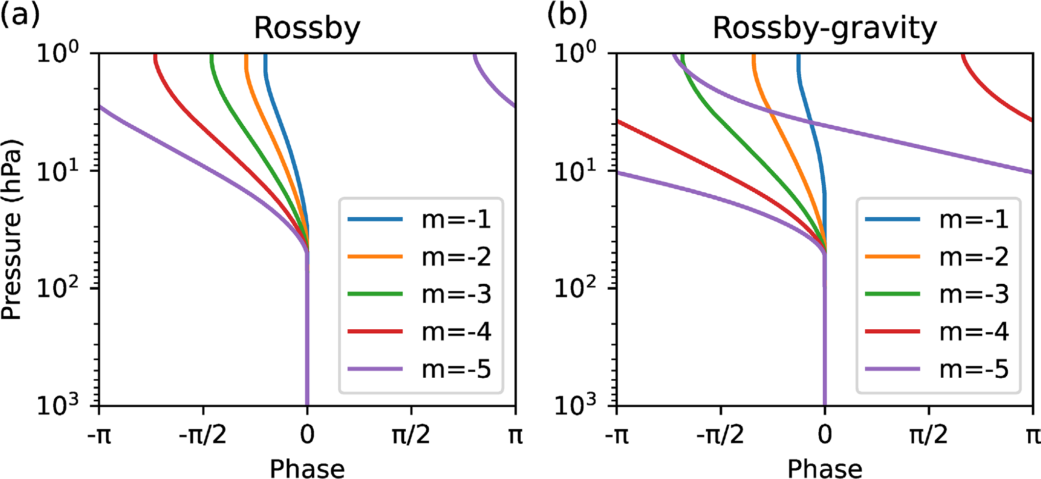
Fig. 14. The vertical structures of the phase for the (a) Rossby and (b) westward Rossby-gravity modes calculated by assuming that the frequencies at any level, determined by the respective dispersion relation in the equatorial β-plain approximation, are equal and using the latitudinally averaged (|ϕ| < 20°) zonal wind and temperature based on the reanalysis data. The zonal wavenumbers (m) are indicated by different colors, the legend of which is shown in each panel.
The effect of the zonal wind on the phase tilt of the modes discussed in the previous paragraph can be seen more clearly in the eigenvalue analysis for the case of a rigid-body rotating wind. Figure 15 shows the vertical structure of the latitudinally averaged (|ϕ| < 20°) geopotential disturbances for the eigenmodes obtained by the eigenvalue analysis using the vertical profile of the global mean temperature based on the reanalysis data and a rigid-body rotation wind defined as follows,

where, we set ΔU =  × 2.5 m s−1. This means that if we take a dimensional log-pressure height as z* = H*z and set H* = × 10 km, the wind speed at the equator increases by 0.25 m s−1 per 1 km of the log-pressure height. Figure 15 shows that for westerly rigid-body rotating winds, the phases of these modes do not change much with altitude, while for easterly winds, they tilt to the west with altitude, and the tilt is more pronounced for the larger wavenumber modes. Comparing the westerly and easterly cases, even if kz2 < 0 and the phase does not change with height at the lower level, the vertical structure of the mode becomes wavy as kz2 > 0 when the easterly wind increases with height, which together with the dissipation effect in the upper region of the model leads to the westward phase tilt. It can also be understood that the degree of westward tilt in the case of easterly winds differs depending on the type of mode and the zonal wavenumber, since the value of kz differs for the same background wind. In Fig. 15, not only the phase but also the amplitude deviates from the Lamb mode structure. Particularly in the case of westerly winds, the amplitudes decrease with height for modes with large zonal wavenumbers. This is because kz2 becomes negative and has a large absolute value for westerly winds, and the amplification rate calculated by (65) becomes negative. Note again, however, that the effect of dissipation is stronger above 10 hPa. To summarize what has been discussed above, particularly for the Rossby-gravity mode and at larger zonal wavenumbers, in the easterly wind regions, the phase is tilted to the west and the amplitude is vertically amplified more than in the Lamb mode structure, while in the westerly wind regions, the phase remains almost constant and the amplitude is more evanescent. In Fig. 8, for the Rossby and westward Rossby-gravity modes with zonal wavenumber 3 or more, the phase is tiled to the west above about 100 hPa, and the amplitude does not increase monotonically with decreasing pressure. Considering the above analysis, the westward phase tilt is due to the easterly winds in the stratospheric equatorial regions, while the amplitude decay with decreasing pressure may be due to the strong mid-latitude westerlies.
4.5 Mechanism for the distortion of latitudinal structures under the influence of background fields
Before closing this section, let us discuss the difference between the latitudinal structures obtained by the eigenvalue analysis and the Hough function structures. The Rossby and westward Rossby-gravity modes with large zonal wavenumbers have slow phase velocities and are sensitive to the zonal wind, which can lead to changes in the latitudinal structures in the same way as the vertical structure has changed. To investigate the effect of the latitudinal profile of the zonal wind on the latitudinal structures of the eigenmodes, the eigenvalue analysis for the zonal wind at the 500 hPa surface based on the reanalysis data with a constant mean depth of 10 km using the barotropic atmospheric model is performed according to the method of Kasahara (1980). Figure 16 shows the latitudinal structures of the geopotential disturbance for the Rossby and westward Rossby-gravity modes obtained by the eigenvalue analysis of the barotropic atmospheric model. For both types of eigenmodes, the absolute values of the amplitudes are larger in the northern hemisphere with notable differences at larger zonal wavenumbers. The characteristics of the amplitudes being larger in the northern hemisphere at larger zonal wavenumbers is consistent with Fig. 7, but the peaks of the amplitude becoming closer to the equator cannot be observed. Therefore, it seems necessary to consider not only the latitudinal profile of the zonal winds but also the vertical structure of the zonal winds in order to understand the amplitude concentration near the equator in the case of large wavenumbers of these modes, as seen in Fig. 7.

5. Summary
Inspired by the comprehensive detection of atmospheric free oscillation modes using the ERA5 reanalysis data by Sakazaki and Hamilton (2020), in the present study a linear eigenvalue analysis of the primitive equations was performed with the zonal mean wind and temperature fields based on the ERA5 data as the basic fields to investigate the effect of background fields on the atmospheric free oscillations with a Lamb mode-like vertical structure. Specifically, the primitive equations in the sigma coordinate were discretized for a given basic field uniform in longitude using a discretization of the three-dimensional spectral method according to Ishioka et al. (2022), with spherical harmonic expansion in the horizontal direction and Legendre polynomial expansion in the sigma direction. The equations were solved numerically as a matrix eigenvalue problem for each zonal wavenumber, and the eigenfrequencies and eigenvectors were obtained. Since such an eigenvalue analysis provides not only Lamb modes deformed by the background field but also spurious eigenmodes due to the finite model top, we introduced a dissipative term in the model for linear eigenvalue analysis, and focusing on the vertical phase structure, latitudinal structure, eigenfrequency, and decay rate in the time direction of each eigenmode, we extracted Lamb-mode-like solutions from these eigenmodes. The zonal mean of the ERA5 reanalysis data from 2011 to 2020 was used as the basic field for the eigenvalue analysis. In addition, to evaluate the influence of the latitudinal/vertical structure of the zonal wind and temperature fields, eigenvalue analyses were also performed for the cases where the zonal wind was set to zero and where the vertical structure of the global mean temperature field was given as the temperature field for comparison. The eigenfrequencies of the eigenmodes obtained by eigenvalue analysis for the zonal mean wind and temperature field were in good agreement with those obtained by spectral analysis in Sakazaki and Hamilton (2020), indicating that the deviations of the eigenfrequencies obtained by the spectral analysis from those obtained by LTE at the equivalent depth of 10 km, which is thought to be the typical equivalent depth of the Lamb mode for the real atmosphere, are mainly due to the zonal wind and temperature variations in the latitudinal and vertical directions. The effect of the zonal wind on the eigenfrequencies of the obtained modes was larger than that of the latitudinal variation of the temperature field for most eigenmodes, but this was not the case for the Rossby mode with zonal wavenumber 1, and for this mode, the effect of the latitudinal temperature variation was dominant. This result was in agreement with that of the spectral analysis of Sakazaki and Hamilton (2020) and the linear eigenvalue analysis of the shallow water equations of Kasahara (1980). The eigenvalue analysis also showed that the effect of the zonal wind on the eigenfrequencies includes not only the Doppler shift effect, but also the effect of the latitudinal derivative of the zonal wind, i.e., the vorticity.
The vertical structures of the geopotential disturbances of the eigenmodes obtained by the eigenvalue analysis were also in good agreement with those obtained in Sakazaki and Hamilton (2020), especially in the sense that two types of differences from the theoretical vertical structure of the Lamb mode for a stationary isothermal atmosphere were observed. One of these differences was that for most of the eigenmodes obtained, the amplitude amplification rate with increasing altitude was smaller than that of the theoretical Lamb mode solution below 100 hPa. This is due to the negative vertical temperature gradient in the troposphere. The other difference was that for the Rossby and westward Rossby-gravity modes with large zonal wavenumbers, the phase was strongly tilted to the west above 100 hPa and the amplitude decay was also observed over a wide range of altitudes. This phase tilt was qualitatively explained using the dispersion relation of the corresponding equatorial wave modes with assuming that the phase speed of each eigenmode should be independent of the altitude. That is, these modes with slow phase speeds must have a wavy vertical structure in the presence of a certain strength of the background easterly wind, while they must have more evanescent vertical structures in the westerly wind regions than that for the theoretical Lamb mode solution for a stationary isothermal atmosphere. The effect of the background wind direction on the vertical structure of the eigenmodes was similarly explained by Salby (1981a, b) using the refractive index of the waves, and the explanation here is not necessarily brand new, but it is unique in that the phase structure was specifically calculated using dispersion relations and compared with the results of the eigenvalue analysis.
The latitudinal structures of the surface pressure fields of the eigenmodes obtained by the eigenvalue analysis in the present study were almost identical to the structures of the corresponding Hough functions for Kelvin modes, gravity modes and eastward propagating Rossby-gravity modes assuming an isothermal stationary atmosphere. However, for the westward Rossby-gravity modes and Rossby modes with slow phase speeds, i.e., large zonal wave numbers, obtained in the present study, the latitudinal distribution of their amplitudes deviated from the theoretical Hough function structure, the equatorial symmetry was broken, and the peaks were shifted more equatorward than in the Hough function case. In Sakazaki and Hamilton (2020), the latitudinal structure of the amplitudes of the eigenmodes extracted from the spectral analysis of the ERA5 data also showed differences from the theoretically obtained structure of the Hough modes. The fact that the differences were large for the westward Rossby-gravity and the Rossby modes with large zonal wavenumbers was consistent with the results of the present study, but the differences from the Hough modes in Sakazaki and Hamilton (2020) were much larger than those obtained in the present study. Moreover, the tendency for the amplitudes in the equatorial regions to be larger than those of the corresponding Hough modes was observed for several gravity modes in Sakazaki and Hamilton (2020), but no such difference was observed for the gravity modes obtained in the present study, and in this respect, too, the results of the present study were inconsistent with those of the spectral analysis of Sakazaki and Hamilton (2020). This discrepancy may be due to the limited duration of the time window analyzed by Sakazaki and Hamilton (2020), or to contamination from other eigenmodes when the latitudinal structure of each mode was determined by regression in Sakazaki and Hamilton (2020), as well as to the influence of the topography and sealand distribution in the real atmosphere.
Finally, let us describe the advantages and points to note of the method of the eigenvalue analysis of the free oscillation modes in the present study in comparison with previous studies. In a sense, the method of the present study is an extension of the two-dimensional eigenvalue analysis for the barotropic atmospheric model of Kasahara (1980) to the three-dimensional primitive equations. Compared to methods such as Geisler and Dickinson (1976), Schoeberl and Clark (1980), and Salby (1981a, b), which searched for resonant solutions by determining the frequency of the forcing, the present method has the advantage that individual eigenmodes can be obtained directly at once, and even if there are several modes with close eigenfrequencies, they can be extracted separately. On the other hand, a point to note of the eigenvalue analysis performed in the present study is that the model used in the present study is based on the formulation of the three-dimensional spectral method of Ishioka et al. (2022), which results in a coarse grid spacing in the upper layers. It is therefore not suitable for investigating the structure of free oscillations in the upper layers of the atmosphere. In addition, a weak dissipation was introduced in the present study to suppress spurious modes due to the finite model top, but this is only for convenience and does not properly correspond to the dissipation in the real atmosphere. Therefore, our future task will be to perform the eigenvalue analysis in a revised three-dimensional model with narrow grid spacing also up to the mesosphere with realistic dissipation and to investigate the frequencies and latitudinal/vertical structures of the Lamb modes affected by a background field. Such an eigenvalue analysis using the model capable of adequately resolving the higher atmospheric regions would allow the analysis of the eigenmodes corresponding to the Pekeris modes detected in Watanabe et al. (2022). Furthermore, in the present study the 10-year averaged zonal wind and temperature fields were used as the basic fields, but more complex latitudinal/vertical structures of the Lamb modes are expected, especially at the solstice condition as shown by Salby (1981b), when the northsouth asymmetry of the basic fields is significant. Given such a background field, where a strong easterly wind appears in the mesosphere, critical layers for Rossby and westward Rossby-gravity modes will appear. In such cases, the eigenmode extraction method as proposed in the present study may not work well. Therefore, as our future work, we should perform an eigenvalue analysis with taking into account the seasonal dependence of the background field and, if necessary, modify the eigenmode extraction method to investigate the seasonal characteristics of the Lamb modes and compare them with those obtained in observational studies. (e.g., Sekido et al. 2024).
Acknowledgments
We thank two anonymous reviewers and the editor, Dr. Masashi Kohma, for their helpful comments. This work was supported by JSPS KAKENHI Grant Numbers 20K04061, 23K25941, 24K07136, and 24K00706. Python and matplotlib were used to draw figures.
References
- Andrews, D. G., J. R. Holton, and C. B. Leovy, 1987: Middle Atmosphere Dynamics. Academic Press, 489 pp.
- Chapman, S., and R. S. Lindzen, 1970: Atmospheric Tides. Springer, 200 pp.
- Geisler, J. E., and R. E. Dickinson, 1976: The five-day wave on a sphere with realistic zonal winds. J. Atmos. Sci., 33, 632–641.
- Hersbach, H., B. Bell, P. Berrisford, S. Hirahara, A. Horányi, J. Muñoz-Sabater, J. Nicolas, C. Peubey, R. Radu, D. Schepers, A. Simmons, C. Soci, S. Abdalla, X. Abellan, G. Balsamo, P. Bechtold, G. Biavati, J. Bidlot, M. Bonavita, G. De Chiara, P. Dahlgren, D. Dee, M. Diamantakis, R. Dragani, J. Flemming, R. Forbes, M. Fuentes, A. Geer, L. Haimberger, S. Healy, R. J. Hogan, E. Hólm, M. Janisková, S. Keeley, P. Laloyaux, P. Lopez, C. Lupu, G. Radnoti, P. de Rosnay, I. Rozum, F. Vamborg, S. Villaume, and J.-N. Thépaut, 2017: Complete ERA5 from 1950: Fifth generation of ECMWF atmospheric reanalyses of the global climate. Copernicus Climate Change Service (C3S) Data Store (CDS). (Accessed on 31 March 2023).
- Hersbach, H., B. Bell, P. Berrisford, S. Hirahara, A. Horányi, J. Muñoz-Sabater, J. Nicolas, C. Peubey, R. Radu, D. Schepers, A. Simmons, C. Soci, S. Abdalla, X. Abellan, G. Balsamo, P. Bechtold, G. Biavati, J. Bidlot, M. Bonavita, G. De Chiara, P. Dahlgren, D. Dee, M. Diamantakis, R. Dragani, J. Flemming, R. Forbes, M. Fuentes, A. Geer, L. Haimberger, S. Healy, R. J. Hogan, E. Hólm, M. Janisková, S. Keeley, P. Laloyaux, P. Lopez, C. Lupu, G. Radnoti, P. de Rosnay, I. Rozum, F. Vamborg, S. Villaume, and J.-N. Thépaut, 2020: The ERA5 global reanalysis. Quart. J. Roy. Meteor. Soc., 146, 1999–2049.
- Hersbach, H., B. Bell, P. Berrisford, G. Biavati, A. Horányi, J. Muñoz Sabater, J. Nicolas, C. Peubey, R. Radu, I. Rozum, D. Schepers, A. Simmons, C. Soci, D. Dee, and J.-N. Thépaut, 2023: ERA5 monthly averaged data on pressure levels from 1940 to present. Copernicus Climate Change Service (C3S) Data Store (CDS), doi:10.24381/cds.6860a573 (Accessed on 1 February 2021).
- Hirota, I., and T. Hirooka, 1984: Normal mode Rossby waves observed in the upper stratosphere. Part I: First symmetric modes of zonal wavenumbers 1 and 2. J. Atmos. Sci., 41, 1253–1267.
- Ishioka, K., 2023: What is the equivalent depth of the Pekeris mode? J. Meteor. Soc. Japan, 101, 139–148.
- Ishioka, K., N. Yamamoto, and M. Fujita, 2022: A formulation of a three-dimensional spectral model for the primitive equations. J. Meteor. Soc. Japan, 100, 445–469.
- Ishizaki, H., T. Sakazaki, and K. Ishioka, 2023: Estimation of the equivalent depth of the Pekeris mode using reanalysis data. J. Meteor. Soc. Japan, 101, 461–469.
- Jones, R. M., 2005: A general dispersion relation for internal gravity waves in the atmosphere or ocean, including baroclinicity, vorticity, and rate of strain. J. Geophys. Res., 110, D22106, doi:10.1029/2004JD005654.
- Kasahara, A., 1976: Normal modes of ultralong waves in the atmosphere. Mon. Wea. Rev., 104, 669–690.
- Kasahara, A., 1980: Effect of zonal flows on the free oscillations of a barotropic atmosphere. J. Atmos. Sci., 37, 917–929.
- Kunze, E., 1985: Near-inertial wave propagation in geostrophic shear. J. Phys. Oceanogr., 15, 544–565
- Lamb, H., 1911: On atmospheric oscillations. Proc. Roy. Soc. A, 84, 551–572.
- Lindzen, R. S., E. S. Batten, and J.-W. Kim, 1968: Oscillations in atmospheres with tops. Mon. Wea. Rev., 96, 133–140.
- Longuet-Higgins, M. S., 1968: The eigenfunctions of Laplace’s tidal equation over sphere. Philos. Trans. Roy. Soc. London, Ser. A, 262, 511–607.
- Matsuno, T., 1966: Quasi-geostrophic motions in the equatorial area. J. Meteor. Soc. Japan, 44, 25–43.
- Pekeris, C. L., 1937: Atmospheric oscillations. Proc. Roy. Soc. A, 158, 650–671.
- Sakazaki, T., and K. Hamilton, 2020: An array of ringing global free modes discovered in tropical surface pressure data. J. Atmos. Sci., 77, 2519–2539.
- Salby, M. L., 1979: On the solution of the homogeneous vertical structure problem for long-period oscillations. J. Atmos. Sci., 36, 2350–2359.
- Salby, M. L., 1981a: Rossby normal modes in nonuniform background configurations. Part I: Simple fields. J. Atmos. Sci., 38, 1803–1826.
- Salby, M. L., 1981b: Rossby normal modes in nonuniform background configurations. Part II: Equinox and solstice conditions. J. Atmos. Sci., 38, 1827–1840.
- Schoeberl, M. R., and J. H. E. Clark, 1980: Resonant planetary waves in a spherical atmosphere. J. Atmos. Sci., 37, 20–28.
- Sekido, H., K. Sato, H. Okui, D. Koshin, and T. Hirooka, 2024: A study of zonal wavenumber 1 Rossby-gravity wave using long-term reanalysis data for the whole neutral atmosphere. J. Meteor. Soc. Japan, 102, 539–553.
- Shepherd, T. G., I. Polichtchouk, R. Hogan, and A. Simmons, 2018: Report on stratosphere task force. ECMWF Technical Memoranda, No. 824, 34 pp.
- Taylor, G. I., 1929: Waves and tides in the atmosphere. Proc. Roy. Soc. A, 126, 169–183.
- Watanabe, S., K. Hamilton, T. Sakazaki, and M. Nakano, 2022: First detection of the Pekeris internal global atmospheric resonance: Evidence from the 2022 Tonga eruption and from global reanalysis data. J. Atmos. Sci., 79, 3027–3043.