How Mountain Geometry Affects Aerosol-Cloud-Precipitation Interactions: Part I. Shallow Convective Clouds

Abstract

This study examines how upslope geometry controls aerosol effects on orographic precipitation through two-dimensional idealized simulations of orographic precipitation from shallow warm convective clouds over a bell-shaped mountain with 1-km height. A total of nine cases are simulated by considering three different prescribed aerosol number concentrations and three different windward-widths of the mountain. For a detailed representation of drop size distributions, the Weather Research and Forecasting (WRF) model that includes a bin microphysics scheme is used with a horizontal grid size of 250 m and 401 terrain-following vertical levels. A higher aerosol number concentration leads to the production of more cloud droplets, inhibiting the growth of cloud droplets into raindrops in the cases with the symmetric mountain (the windward-side half-width a₁ = 10 km). As a result, the total and maximum surface precipitation amounts decrease and the location of the maximum surface precipitation amount shifts downstream. The aerosol effects on orographic precipitation are more clearly seen in the cases with the narrow windward-width (a₁ = 5 km) compared to the cases with the symmetric mountain and the wide windward-width (a₁ = 20 km). In the cases with the narrow windward-width, the steep upslope generates strong convection with a short advection timescale (∼ 600 s), resulting in more precipitation being concentrated over a narrow area of the mountain downslope compared to the cases with the symmetric mountain and the wide windward-width. On the other hand, in the cases with the wide windward-width, the gentle upslope generates weak convection with a sufficiently long advection timescale (∼ 2400 s) so that a large portion of liquid drops precipitates out on the wide mountain upslope before reaching the peak.

1. Introduction

Aerosol particles control precipitation characteristics by acting as cloud condensation nuclei (CCN) or ice nuclei (IN). Rosenfeld (1999) and Andreae et al. (2004) showed that smoke aerosols from forest fires can inhibit rainfall. Urban pollution also suppresses downstream rainfall and snowfall (Rosenfeld 2000). The precipitation-suppressing effect of aerosol particles is reported in various numerical studies (e.g., Givati and Rosenfeld 2004; Khain et al. 2004; Xie et al. 2013). These numerical studies show that precipitation is suppressed in an aerosol-rich condition under which the cloud droplet distribution favors small sized drops. Many observational and numerical studies have shown that air pollution in mountainous areas, such as the western United States, inland of Israel, and northern China, also suppresses precipitation (Givati and Rosenfeld 2004; Jirak and Cotton 2006; Rosenfeld and Givati 2006; Rosenfeld et al. 2007; Guo et al. 2014).

Mountain geometry and environmental factors can affect the convective development of orographic clouds (Dudis 1972; Durran and Klemp 1982; Hernandez-Duenas et al. 2015). Cannon et al. (2012, 2014) numerically studied the conditions for generations of complex orographic convection. Under convection-prone conditions, orographic convection constructs a cellular or a banded structure (Kirshbaum and Durran 2004, 2005). Well-developed orographic convection is reported in many observational studies using field campaign data (Smith et al. 2012; Minder et al. 2013; Wang and Kirshbaum 2015) and in many numerical studies using high-resolution models (Kirshbaum and Smith 2009; Panosetti et al. 2016; Sever and Lin 2017).

Precipitation over mountainous areas has long been a topic of investigation (Barros and Lettenmaier 1994; Roe 2005; Houze 2012). Many theoretical methods were designed to systematically study orographic precipitation (e.g., Smith and Lin 1982; Lin 1986; Smith and Barstad 2004). It is, however, difficult to make a detailed generalization about the characteristics of orographic precipitation because orographic precipitation is affected by a complex web of interrelated factors including microphysical processes, mountain geometry, and background static stability and wind speed (Chu and Lin 2000; Colle 2004; Sever and Lin 2017; Morales et al. 2018). Colle (2004), Pathirana et al. (2005), and Roe and Baker (2006) examined the sensitivity of orographic precipitation to changes in mountain geometry (mountain height and width) and basic wind speed. These studies assessed the importance of mountain barrier effects and the roles that mountain waves play in shallow orographic precipitation from a macroscopic viewpoint. The mountain height and width modify the strength of orographic convection by controlling upslope steepness. A narrow mountain with a steep upslope sometimes leads to more precipitation on the leeside of the mountain (Roe and Baker 2006). However, depending on environmental factors, a wide mountain with a gentle upslope can also result in more precipitation on the leeside of the mountain (Pathirana et al. 2005). To systematically examine the effects of upslope steepness on orographic precipitation, asymmetric mountains with different upslope steepnesses but fixed downslope geometry are considered in this study, focusing on the combined effects of macroscopic features and microphysical processes in generation and development of orographic precipitation.

Characterizing the effects of aerosol particles on orographic precipitation is a challenge because there are many different complicating factors involved such as dynamical and microphysical processes as well as the influence of mountain geometry and environmental factors. Several studies have numerically examined aerosol effects on orographic precipitation using bulk microphysics models and have shown that aerosols reduce the total precipitation amount over mountains (Creamean et al. 2015; Yang et al. 2016). Nugent et al. (2016) studied aerosol effects on orographic-convective precipitation with and without the basic wind using an aerosol-aware bulk microphysics model. To understand the effects aerosols have on precipitation from convective orographic clouds more clearly, numerical simulations using a bin microphysics model, which predicts the number concentration of each hydrometeor in each size bin (e.g., Khain et al. 2000; Lynn et al. 2005a, b), are desirable. Studies using bin microphysics models have provided some insights into the details about the microphysical processes in orographic precipitation influenced by aerosols, including the evolution of the size distributions of hydrometeors (Lynn et al. 2007; Xue et al. 2010; Xiao et al. 2014, 2015). Nevertheless, aerosol effects on orographic precipitation from cellular or banded convective clouds remain poorly understood.

Multitudes of bin and bulk microphysics schemes are available for simulating clouds and precipitation. The detailed representation of microphysical processes in bin microphysics schemes provides a greater accuracy in model results compared to bulk microphysics schemes. The downside is that the models equipped with bin microphysics schemes require much more computational resources. For this reason, few studies have used models with bin microphysics schemes. Khain et al. (2005) used a bin microphysics model to study aerosol effects on deep convective precipitation. Bin microphysics models have also been used to study aerosol effects on shallow convective precipitation (Wyszogrodzky et al. 2011; Blyth et al. 2013; Grabowski et al. 2015; Lee et al. 2015). Related to the growth speeds of hydrometeors, aerosol effects on orographic precipitation and how they are affected by various mountain geometries are still poorly understood. Because of the inherent advantages that bin microphysics schemes have over bulk microphysics schemes, a bin microphysics scheme is more appropriate for studying this problem.

In this study, we examine how upslope geometry controls aerosol effects on orographic precipitation from shallow convective clouds using a bin microphysics model in order to further our understanding of aerosol-cloud-precipitation interactions in mountainous regions. Section 2 describes the numerical model and the simulation design. The simulation results are presented and discussed in Section 3. A summary and conclusions are given in Section 4.

2. Experimental design

2.1 Model description

The numerical model used in this study is the Weather Research and Forecasting (WRF) model, version 3.6.1, coupled with the bin microphysics scheme of the Hebrew University Cloud Model (HUCM) (Skamarock et al. 2008; Lee and Baik 2016). The detailed description of HUCM is given in Khain and Sednev (1996) and Khain et al. (2000, 2004). The WRF-bin model considers 43 mass-doubling bins. Following Khain et al. (2000) and Lee et al. (2014), the initial aerosol size distribution N (r_a) is specified as   

where r_a is the aerosol radius, N₀ is the aerosol number concentration (here, CCN number concentration) at 1 % supersaturation, and k is a constant (0.8 in this study). A = 2σ/(ρ_wR_vT) is the coefficient related to the curvature effect, where σ is the surface tension of the liquid drop, ρ_w is the density of liquid water, R_v is the gas constant of water vapor, and T is the temperature. B = iM_wρ_a/(ρ_wM_a) is the coefficient related to the solution effect, where i is the degree of ionic dissociation, M_w is the molecular weight of water, ρ_a is the density of the aerosol (solute), and M_a is the molecular weight of the aerosol. In this study, NaCl is considered as the aerosol material. Note that the type of aerosol particle only affects the ratio of activated drop number concentration to the total aerosol number concentration, so it does not alter the qualitative conclusions of this study. The radius of the largest aerosol is 2 µm. The initial aerosol number concentration is constant up to the 2-km height and then decreases exponentially with height with an e-folding height of 2 km. In the WRF-bin model, a liquid drop larger (smaller) than r* = 40 µm is categorized as a raindrop (cloud droplet).

2.2 Simulation settings

To examine orographic precipitation, we construct two-dimensional simulations (Fig. 1a). A bell-shaped mountain is considered, whose height h is given by   

where h_m (= 1 km) is the maximum height and a is the half-width of the bell-shaped mountain. The leeward-width is constant (a = a₂ = 10 km for x ≥ 0 km), while the windward-width determined by a = a₁ (for x < 0 km) varies. We classify simulation cases into three groups based on N₀. The clean (CLN), control (CNT), and polluted (PLT) cases correspond to N₀ = 100, 500, and 2500 cm⁻³, respectively. These CCN number concentrations fall in a range found in real measurements (Andreae 2009; Benmoshe and Khain 2014; Lee et al. 2014). Based on the windward-width of the mountain a₁, which determines the upslope steepness, each group is subdivided into three cases (Table 1). The n and the w at the end of each case title indicate the narrow (a₁ = 5 km) and wide (a₁ = 20 km) windward-width of the mountain, respectively. Here, we use the windward-width of the mountain rather than the upslope steepness to control the mountain geometry because the windward-width of the mountain captures in a single parameter both the upslope steepness and the distance over which cellular convective clouds travel until they reach the mountain peak. In this study, a uniform background wind speed with U = 10 m s⁻¹ is used.

Fig. 1.

(a) Schematic diagram of the simulation configuration. The dashed (dotted) line is for the case of narrow (wide) windward-width of the mountain. (b) Skew T-log p diagram, (c) relative humidity profile, and (d) equivalent potential temperature (black solid) and dew-point equivalent potential temperature (blue dashed) profiles of the sounding data at Osan, South Korea at 00 UTC 19 September 2012. The green dashed line in (b) indicates the moist adiabat above the LCL.

Table 1.Names and corresponding aerosol number concentrations N₀ and windward-width of the mountain a₁ for the nine cases.

Thermodynamic sounding data at Osan, South Korea at 00 UTC on 19 September 2012 are used to simulate orographic precipitation from shallow convective clouds. Figures 1b, 1c, and 1d show the skew T-log p diagram, relative humidity profile, and equivalent potential temperature and dew-point equivalent potential temperature profiles of the sounding data, respectively. Figure 1b gives basic information about the thermodynamic structure. The near-surface temperature is 17.8°C, and the near-surface relative humidity is 86 %. Orographic clouds are generated at the lifting condensation level (LCL) of 409 m, which is below the mountain top. The horizontal location at which h(x) = z_LCL is x = x_LCL ∼ −1.2a₁. The level of free convection (LFC) is 1476 m. Above the equilibrium level (EL) of 2788 m, a strong inversion layer is present, which prevents convective developments there. The temperature at the EL is 2.2°C, so we consider warm microphysical processes only.

The horizontal domain size is 1000 km with a grid size of 250 m. The open boundary condition is applied in the x-direction. The vertical domain size is 15 km, with a 5-km-depth sponge layer between z = 10 km and 15 km. There are 401 terrain-following levels in the vertical direction. The WRF-bin model is integrated for 12 h with a time step of 0.6 s. The data save interval is 10 min, which is shorter than the typical timescale of orographic-convective precipitation. The spatial resolution in this study is appropriate for resolving the active cellular/banded convection associated with orographic-convective precipitation (Kirshbaum and Durran 2004; Kirshbaum and Smith 2008). Parameterizations of shortwave/longwave radiation, boundary layer, and surface processes are turned off in the simulations.

3. Results and discussion

3.1 General characteristics of the simulated orographic precipitation

A comparison of the timescales for orographic precipitation can give us a clue regarding the relative importance of given orographic-precipitation-related processes (Jiang and Smith 2003). Miglietta and Rotunno (2009) and Cannon et al. (2012) compared the convection timescale τ_c with the advection timescale τ_a which are defined as   

  

where H_c is the vertical length scale of convection (z_EL − z_LCL = 2379 m in this study) and CAPE stands for the convective available potential energy. Note that CAPE (28 J kg⁻¹) is calculated from the LFC, not from the LCL. In the case with a₁ = 10 km and U = 10 m s⁻¹, τ_c = 450 s and τ_a = 1200 s. This means that the orographic clouds generated at the LCL can be fully developed up to the EL before they reach the top of the mountain (see the green dashed line in Fig. 1b and the vertical profiles in Fig. 1d). In this case, the condensational heating provides additional energy, and the updrafts over the upslope associated with mountain waves strengthen the upward motion in the convective clouds.

Potential instability, or the sign of dθ_e/dz, determines the type of orographic clouds (stratiform or convective). Kirshbaum and Durran (2004) showed that convection may not develop even in the region of negative dθ_e/dz. They suggested that N_m², where N_m is the moist Brunt-Väisälä frequency, can discriminate the possibility of convective development (unstable when N_m² < 0). Both formulas introduced by Lalas and Einaudi (1974) and Durran and Klemp (1982) include −dq_w/dz (q_w = total water mixing ratio) which acts to reduce N_m². As shown in Fig. 1d, dθ_e/dz is less than −5 K km⁻¹ in two layers, z = (0.7 km, 1.3 km) and (2.6 km, 3.0 km). Because the relative humidity steeply decreases in the layer z = (2.6 km, 3.0 km), the development of convection there can be weak or inhibited even though dθ_e/dz < 0. This strong stabilizing in the layer z = (2.6 km, 3.0 km) can also be seen from the dew-point equivalent potential temperature profile (blue dashed) in Fig. 1d. On the other hand, convective cells can develop in the layer z = (0.7 km, 1.3 km) given the much smaller relative humidity gradient there.

Cloud droplets in orographic shallow convective clouds grow primarily through collision/coalescence. Over the mountain upslope, strong orographic uplift and strong convective updrafts enhance the growth of cloud droplets into large raindrops. Large raindrops with sufficiently high terminal velocities can fall and reach the surface. A large portion of liquid drops can pass over the mountain peak by advection so that surface precipitation can be concentrated on the mountain downslope. Downdrafts associated with mountain waves help the sedimentation of liquid drops by accelerating their fall speeds, but they also enhance the evaporation of cloud droplets and small raindrops. From t ∼ 6 h, the overall patterns of the flow and the hydrometeor distributions reach a quasi-steady state. Hereafter, the snapshots at t = 6 h and the accumulated or averaged variables in the range t = 6–12 h are mainly used for analysis.

3.2 Aerosol effects on orographic precipitation

Figures 2 and 3 show the fields of vertical velocity, cloud water mixing ratio, and rainwater mixing ratio at t = 1 and 6 h, respectively, in CLN, CNT, and PLT. These figures show that as N₀ gets larger, the cloud water mixing ratio gets higher, while the rainwater mixing ratio gets lower. At t = 1 h, the orographic convective clouds are deeper in PLT than in CLN and CNT because the condensational heating is stronger in PLT. At t = 6 h, the vertical velocity over the leeside is strongest in CLN. In PLT, orographic clouds are distributed farther downstream compared to those in CLN and CNT.

Fig. 2.

Fields of vertical velocity (shaded), cloud water mixing ratio (green contours), and rainwater mixing ratio (black contours) at t = 1 h in (a) CLN, (b) CNT, and (c) PLT. The contour interval is 0.4 g kg⁻¹, and the maximum values of contour lines for cloud water and rainwater mixing ratios in each panel are presented in the bottom boxes.

Fig. 3.

The same as Fig. 2, but at t = 6 h.

Figure 4 shows the horizontal distributions of surface precipitation amount accumulated from t = 6 to 12 h in CLN, CNT, and PLT. The accumulated surface precipitation amount is distributed more broadly downstream of the mountain peak in PLT than in CLN and CNT. The total surface precipitation amount summed over the entire domain P_tot, the local maximum of the 6-h accumulated surface precipitation amount P_max, and the location at which P_max occurs x_max are listed in Table 2. The total surface precipitation amount decreases as N₀ increases. The maximum surface precipitation amount in CLN is 1.8 and 4.9 times the amounts in CNT and PLT, respectively.

Fig. 4.

Horizontal distributions of surface precipitation amount accumulated from t = 6 to 12 h in the cases with a₁ = 10 km. The dash-dotted line indicates the x-location of the mountain peak.

Table 2.Total 6-h accumulated surface precipitation amount summed over the entire domain P_tot, the maximum 6-h accumulated surface precipitation amount P_max, and the location at which P_max occurs x_max in the nine cases.

An increase in the CCN number concentration enhances activation into cloud droplets and results in increased number concentration, decreased average size, and increased total surface area of liquid drops. Therefore, the growth of cloud droplets into raindrops is reduced (Khain et al. 2004, 2005; Lynn et al. 2007; Xiao et al. 2014, 2015). As a result, the total surface precipitation amount is smaller in PLT than in CLN and CNT. In PLT, a large portion of liquid drops are advected downstream of the mountain peak, and the surface precipitation is distributed more broadly there. In CLN, on the other hand, the active growth of cloud drops into raindrops causes a rapid sedimentation of liquid drops.

Table 3 lists the 6-h averaged condensation and evaporation rates integrated over the mountain upslope and downslope, each spanning 100 km in the horizontal direction and 3 km in the vertical direction. The 6-h averaged surface precipitation rates integrated on the mountain upslope and downslope are also listed. Condensation is more active than evaporation over the mountain upslope, and evaporation is more active than condensation over the mountain downslope. Concerning the condensation rate over both mountain upslope and downslope, the differences between PLT and CNT are greater than those between CNT and CLN. This is also true for the evaporation rate. The liquid drops generated over the mountain upslope fall on the ground or are advected toward the leeward side of the mountain. The precipitation rates on the mountain downslope are 89 %, 195 %, and 445 % of those on the mountain upslope in CLN, CNT, and PLT, respectively. Note that more precipitation occurs on the mountain upslope than on the mountain downslope in CLN, while the opposite holds for CNT and PLT.

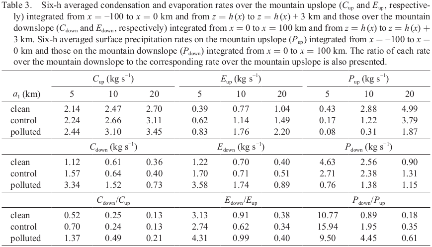
Table 3.Six-h averaged condensation and evaporation rates over the mountain upslope (C_up and E_up, respectively) integrated from x = −100 to x = 0 km and from z = h (x) to z = h (x) + 3 km and those over the mountain downslope (C_down and E_down, respectively) integrated from x = 0 to x = 100 km and from z = h (x) to z = h (x) + 3 km. Six-h averaged surface precipitation rates on the mountain upslope (P_up) integrated from x = −100 to x = 0 km and those on the mountain downslope (P_down) integrated from x = 0 to x = 100 km. The ratio of each rate over the mountain downslope to the corresponding rate over the mountain upslope is also presented.

To analyze the size distribution of the liquid drops that pass over the mountain peak, we calculate the advection rate of liquid drops over the mountain peak (Fig. 5) as follows:   

where r is the drop radius, t₁ = 6 h, t₂ = 12 h, T = t₁ − t₂, H (= 3 km) is the vertical depth of the integration, q_l is the liquid water mixing ratio, and u is the horizontal wind velocity. Note that ρ_w is the density of liquid water. As discussed, most of the liquid drops are cloud droplets in PLT. Compared to CLN and CNT, the average size of cloud droplets in PLT is smaller. In CLN, raindrops take up more than half the mass of all advected liquid drops. The faster growth of cloud droplets in CLN means that the average size of raindrops in CLN is larger than that in CNT or PLT. The size distributions of liquid drops exhibit double-peak patterns; one peak in the size range of cloud droplets and the other peak in the size range of raindrops (Fig. 5). In CLN, a relatively large mass of drops falls into the size spectrum between the two peaks of the size distribution—an indication that the growth from cloud droplets to raindrops is active in convective clouds near the mountain peak.

Fig. 5.

Six-h averaged advection rates of liquid drops over the mountain peak integrated from z = h(x) to z = h(x) + 3 km as a function of drop radius in the cases with a₁ = 10 km. The dash-dotted line indicates the size-boundary between cloud droplets and raindrops (r* = 40 µm).

Figure 6 shows the 6-h averaged mass-size distributions of liquid drops in CLN and PLT along with the difference in the 6-h averaged mass-size distribution of liquid drops between PLT and CLN as a function of horizontal location and as a function of height above the terrain surface. Here and hereafter, the mass-size distributions are normalized by dlnr. Because the initial CCN number concentration in PLT is 25 times higher than that in CLN, the concentration of very small droplets over the entire domain is clearly higher in PLT than in CLN. Figures 6a, 6c, and 6e show that the size of the cloud droplets distributed over both the mountain upslope and downslope is smaller in PLT than in CLN. Where the cloud droplets are larger in CLN than in PLT is concentrated mainly in the horizontally narrow region over the mountain upslope (Figs. 6a, e). Compared to CLN, the mass-size distributions of liquid drops of convective clouds are vertically more elongated in PLT, which is caused by the strong latent heat release from the active condensation associated with increased total surface area of liquid drops due to the large number of CCN in PLT (Figs. 2a, c, 6b, d). Most cloud droplets are in the convection region or near the surface, and their size is much smaller in PLT than in CLN. In PLT, small raindrops get even smaller through evaporation as they fall. As a result, many raindrops in PLT are located at high altitudes. Near the surface, the mass of raindrops is greater in CLN than in PLT (Figs. 6b, d, f).

Fig. 6.

Six-h averaged mass-size distributions of liquid drop (g kg⁻¹) in (a, b) CLN and (c, d) PLT and (e, f) difference in the 6-h averaged mass-size distributions of liquid drops between PLT and CLN as a function of (a, c, e) horizontal location and as a function of (b, d, f) height above the terrain surface. The values at grid points are summed in (a, c) the z-direction and (b, d) the x-direction. The dashed line indicates the size-boundary between cloud droplets and raindrops (r* = 40 µm).

3.3 Sensitivity of aerosol effects on orographic precipitation to upslope steepness

The half-width of the windward side of the mountain controls the upslope steepness and the advection timescale (Eq. 4). Figure 7 is the same as Fig. 3 except for the upslope steepness of the mountain. Here, we consider the cases with the narrow windward-width (CLNn, CNTn, and PLTn), where the steeper upslope rapidly lifts moist air. The rapid uplift results in an increase in the maximum surface precipitation amount in CLNn and CNTn (Table 2). In all three cases with the narrow windward-width, the small advection timescale (τ_a ∼ 600 s) causes the condensation, evaporation, and precipitation rates over the mountain upslope to decrease (Table 3). Recall that in PLT, the relatively large number of CCN causes both the increase in the rate of condensation into cloud droplets and the delay of growth of cloud droplets into raindrops. In PLTn, compared to CLNn and CNTn, the shortened advection time severely reduces the chance for liquid drops to grow because they evaporate rapidly once the downdrafts associated with mountain waves take effect, even though the condensation rates over the mountain upslope and downslope are increased with increasing N₀ (Table 3). In this way, the aerosol effects are more clearly seen in the cases with the narrow windward-width (Table 2, Fig. 9a). Note that the aerosol effects here refer to the decrease in the total surface precipitation amount and the downstream shift of the horizontal location of the maximum surface precipitation amount.

Fig. 7.

The same as Fig. 3 except for (a) CLNn, (b) CNTn, and (c) PLTn.

Fig. 8.

The same as Fig. 3 except for (a) CLNw, (b) CNTw, and (c) PLTw.

Fig. 9.

The same as Fig. 4 except for (a) a₁ = 5 km and (b) a₁ = 20 km.

Figure 8 is the same as Fig. 3, except now we consider the cases with the wide windward-width. In CLNw, CNTw, and PLTw, the relatively long horizontal length of the mountain upslope affords greater chances for cloud droplets to grow and for liquid drops to fall onto the mountain upslope over a longer advection timescale (τ_a ∼ 2400 s). For this reason, a large portion of drops are precipitated out onto the surface before reaching the mountain peak via advection. The horizontal distributions of the accumulated surface precipitation amount are broader over the mountain upslope than over the mountain downslope (Fig. 9b). The total amount of the accumulated surface precipitation amount over the mountain upslope is larger than that over the mountain downslope. In all three wide windward-width cases, x_max is located on the mountain upslope (Table 2). The slower growth of cloud droplets in PLTw results in a smaller total surface precipitation amount, and the location of the maximum surface precipitation amount is farther downstream compared to CLNw and CNTw (Table 2). Compared to the cases with the narrow windward-width and the symmetric mountain, the decrease in the maximum surface precipitation amount with increasing N₀ is smaller in the cases with the wide windward-width.

The advection rates of liquid drops over the mountain peak as a function of drop radius in the cases with the narrow windward-width are presented in Fig. 10a. Having a narrower windward-width than the symmetric mountain causes a stronger uplift by the steeper upslope, which results in a larger number of cloud droplets being generated and advected over the mountain peak, although the smaller advection timescale limits their growth into large raindrops. The raindrop advection rate peaks at a smaller drop size in CNTn than in CLNn and PLTn. The size distribution favoring large raindrops in CLNn is due to the low aerosol number concentration. On the other hand, PLTn has the size distribution with larger raindrops than CNTn, because the slow growth of raindrops reduces the consumption of large raindrops via sedimentation. A detailed analysis regarding the liquid drop growth in the limited advection timescale will be given later.

Fig. 10.

The same as Fig. 5 except for (a) a₁ = 5 km and (b) a₁ = 20 km.

In the cases with the wide windward-width (Fig. 10b), the lengthy upslope provides a sufficient amount of time for cloud droplets to grow so that a large portion of raindrops are already precipitated out onto the wide mountain upslope. As a result, the amount of drops that are advected over the mountain peak is small in all wide windward-width cases. In these cases, the raindrop advection rate peaks at a larger drop size in CNTw than in CLNw and PLTw. In CLNw, the faster growth of liquid drops results in more precipitation on the mountain upslope and the decrease in the advected large-sized raindrops over the mountain peak. Compared to CNTw, the raindrop amount in PLTw peaks at a smaller size because of the higher aerosol number concentration, and the smaller rate of surface precipitation on the mountain upslope results in a higher raindrop advection rate over the mountain peak. The double-peak size distribution pattern of the advected liquid drops clearly appears in PLTw, like in CLN and CNT with the symmetric mountain (Fig. 5), but such a pattern is not as clearly seen in CLNn, CNTn, PLTn, CLNw, and CNTw (Fig. 10). Note that unlike in Fig. 5, the ranking among the raindrop advection rates corresponding to the three different aerosol number concentrations in Fig. 10 does not stay consistent.

Some amount of time is needed if the condensates generated near x ∼ x_LCL are to grow into raindrops. Likewise, some amount of time is needed for the raindrops to grow into large raindrops with a terminal velocity high enough for the falling drops to reach the surface in the limited advection timescale. These two amounts of time needed are related to the autoconversion timescale and the sedimentation timescale, respectively. In many autoconversion parameterizations used in bulk schemes, the autoconversion timescale is regarded as one of the model-inherent characteristics rather than being a situation-dependent scale (Kessler 1969; Long 1974; Manton and Cotton 1977). Berry and Reinhardt (1974a, b) suggested a characteristic autoconversion timescale based on the results obtained using a bin stochastic collection model. The characteristic time scale in their study is determined by the time at which the characteristic radius of liquid drops first reaches r* = 50 µm. Many studies have since applied and improved Berry and Reinhardt's method (see Gilmore and Straka 2008).

In this study, we calculate the horizontal distribution of the mean size of liquid drops and compare among the cases the locations at which the mean size of liquid drops first reaches r* = 40 µm. This is to estimate how fast the condensates grow during the advection. Likewise, in order to estimate how fast raindrops grow into large raindrops with a sufficiently high terminal velocity, r_T, the mean size distribution of raindrops is also calculated. It is rather difficult to explicitly define the location at which the mean size of raindrops first reaches r_T because raindrops are distributed over a broad range in both the horizontal and vertical directions with various size distributions as shown in Fig. 6. To circumvent this issue, we arbitrarily set r_T = 200 µm. Raindrops of this size are large enough to have a sufficiently high terminal velocity of ∼ 1.6 m s⁻¹, yet at the same time are small enough for growing raindrops in all cases to catch up to that size. The horizontal distributions of the mean radii of liquid drops r̄_l (x) and raindrops r̄_r (x) are obtained as follows:   

  

where t₃ and t₄ are the initial and final times considered for time averaging, respectively, and T′ = t₄ − t₃.

Figures 11 and 12 show the horizontal distributions of r̄_l (x) and r̄_r (x), respectively (dashed lines). Here, the time integration is taken from t = 0 to 1 h (t₃ = 0 h and t₄ = 1 h), not from t = 6 to 12 h. This is because after t = 6 h, the horizontal and vertical structures of the atmosphere are already considerably disturbed through dynamical and microphysical processes during the precipitation event, and the orographic clouds are already extended upstream, making an intuitive comparison with the advection timescale difficult. The mean size distribution is flattened using the locally weighted regression fitting method with 0.1 as the smoothing parameter (Cleveland and Devlin 1988); this enables us to better recognize the general features from the complex cellular convective clouds.

Fig. 11.

Horizontal distributions of the mean radius of liquid drops calculated using Eq. (6a) in the cases with a₁ = (a) 5 km, (b) 10 km, and (c) 20 km (dashed lines). Solid lines indicate the smoothed horizontal distributions. The horizontal and vertical dash-dotted lines indicate the size-boundary between cloud droplets and raindrops (r* = 40 µm) and the x-location of the mountain peak, respectively.

Fig. 12.

The same as Fig. 11 except for the raindrops and Eq. (6b). The horizontal dash-dotted line indicates r = 200 µm.

In the cases with the symmetric mountain, the location x* at which r̄_l (x) first reaches r* is −9.00, −7.25, and 3.00 km and the location x_T at which r̄_r (x) first reaches r_T is −6.75, −1.25, and 11.75 km in CLN, CNT, and PLT, respectively. If we define the autoconversion timescale by τ* = (x* − x_LCL)/U and the sedimentation timescale by τ_T = (x_T − x*)/U (see Fig. 13), it follows that τ* = 300, 475, and 1500 s and τ_T = 225, 600, and 875 s in CLN, CNT, and PLT, respectively. Table 4 shows the collection of x*, τ*, x_T, and τ_T in the nine cases. In CLN and CNT, condensates sufficiently grow into raindrops and the raindrops sufficiently grow into raindrops with r = r_T within the advection timescale τ_a (τ* + τ_T < τ_a = 1200 s), and x_max is located near the mountain peak. The slow growth of condensates in PLT (τ* > τ_a) results in x_max being far on the leeside of the mountain (Fig. 4, Table 2) and a small advection rate of raindrops over the mountain peak (Fig. 5).

Fig. 13.

Schematics for calculating the autoconversion timescale τ* = (x* − x_LCL)/U and the sedimentation timescale τ_T = (x_T − x*)/U. The location at which r̄_l (x) first reaches the size-boundary between cloud droplets and raindrops (r* = 40 µm) is x*. The location at which r̄_r (x) first reaches r_T = 200 µm is x_T. The smallest drop radius r₀ is 2 µm in the bin microphysics model used in this study. Here, the symmetric mountain is depicted for illustration purpose.

Table 4.The location x* at which r̄_l(x) first reaches r* = 40 µm, the location x_T at which r̄_r (x) first reaches r_T = 200 µm, the autoconversion timescale τ* = (x* − x_LCL)/U, and the sedimentation timescale τ_T = (x_T − x*)/_U in the nine cases.

In the cases with the narrow windward-width, x* = 1.50, 4.25, and 6.00 km, x_T = 6.75, 6.75, and 6.25 km, τ* = 750, 1025, and 1200 s, and τ_T = 525, 250, and 25 s in CLNn, CNTn, and PLTn, respectively. In these cases, the growth of condensates is very slow and r̄_l (x) cannot reach r* within the advection timescale (τ* > τ_a = 600 s). For this reason, the advection rate of raindrops over the mountain peak is very small (Fig. 10a). Moreover, the growth of cloud droplets (small liquid drops) suffers from downdrafts associated with mountain waves over the mountain downslope so that the growth of liquid drops is further delayed. The strong convection due to the active condensation in PLTn (Table 3) results in the fast growth of raindrops (large liquid drops) toward r_T over the mountain downslope (Fig. 12a). However, a large portion of the liquid drops is still small in size (Fig. 10a). As a result, a large mass content of the small-sized drops evaporates over the mountain downslope (Table 3). Therefore, the total surface precipitation amount is much smaller in PLTn than CLNn and CNTn, even though the differences in the mean size of liquid drops among the three cases with the narrow windward-width are less drastic compared to those among the cases with the symmetric mountain and the wide windward-width. The downstream shift of the peak in the mean size distribution of liquid drops with increasing N₀ is seen in Figs. 11a and 11b.

In the cases with the wide windward-width, x* = −21.75, −18.00, and −6.75 km, x_T = −15.50, −14.25, and −4.25 km, τ* = 225, 600, and 1725 s, and τ_T = 625, 375, and 250 s in CLNw, CNTw, and PLTw, respectively. In these cases, liquid drops can sufficiently grow into large raindrops within the advection timescale (τ* + τ_T < τ_a = 2400 s) and x_max is located at the mountain upslope. As presented earlier, a great portion of liquid drops are precipitated out over the mountain upslope before reaching the mountain peak in CLNw and CNTw. For this reason, in CLNw and CNTw, the mean size of raindrops peaks before reaching the mountain peak and starts decreasing in the downstream direction with the advection rate of raindrops over the mountain peak being fairly small (Fig. 10b). On the other hand, in the cases with the narrow windward-width, the mean size of raindrops continues to increase near the mountain peak and reaches the peak size over the mountain downslope (Fig. 12). In PLTw, the decreasing trend begins near the mountain peak (Fig. 12c). For this reason, the accumulated surface precipitation amount decreases more slowly in PLTw compared to CLNw and CNTw (Fig. 9b).

Figure 14 presents the differences in mass-size distribution between PLTn and CLNn and between PLTw and CLNw as a function of horizontal location and as a function of height above the terrain surface. In the cases with the narrow windward-width, the steeper upslope generates stronger convection so that the maximum surface precipitation amount in the clean and control cases is larger compared to the cases with the symmetric mountain and the wide windward-width (Table 2). There is an outstanding positive difference between PLTn and CLNn (Fig. 14b). Although the advection rate of raindrops over the mountain peak is lower due to the insufficient advection time in the cases with the narrow windward-width than in the cases with the symmetric mountain (Figs. 5, 10a), the cloud droplets further grow into raindrops even over the mountain downslope. Precipitation in PLTn is distributed farther downstream because the average size of liquid drops is relatively small in PLTn; thus, a longer advection time is needed for the cloud droplets in PLTn to grow into large raindrops that have sufficiently high terminal velocities to precipitate out. As a result, PLTn shows a clear downstream shift of the location of the maximum surface precipitation amount, even though the raindrop size difference between PLTn and CLNn is smaller than that between PLT and CLN (Figs. 6e, 12a, b, 14a).

Fig. 14.

The same as Figs. 6e and 6f except for (a, b) PLTn and CLNn and (c, d) PLTw and CLNw.

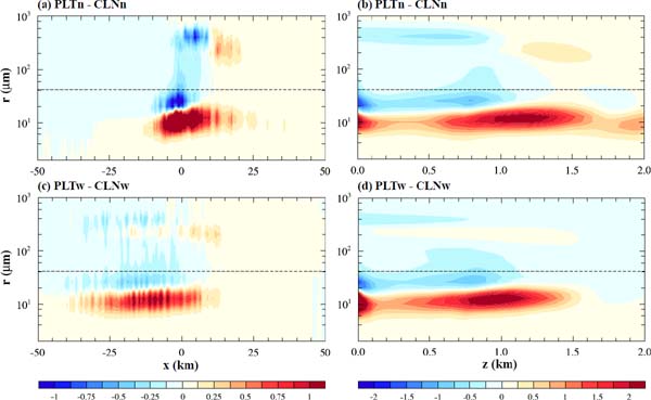
In the cases with the wide windward-width, the convective clouds exhibit vertically less elongated mass-size distributions compared to the cases with the narrow windward-width (Figs. 14b, d). Compared to the cases with the narrow windward-width and the symmetric mountain, the size distributions of cloud droplets and raindrops are clearly distinguishable between PLTw and CLNw (Fig. 14c) because in the wide windward-width cases, the generation, growth, and sedimentation of liquid drops occur over the longer horizontal distance upslope. Because most of the liquid drops are precipitated out over the wide upslope, the aerosol effects are not so obvious.

4. Summary and conclusions

Through the numerical simulations using the WRF model that includes a bin microphysics scheme, this study examined how upslope geometry controls aerosol effects on orographic precipitation from shallow convective clouds. Forced uplift by a bell-shaped mountain generates orographic precipitation. By changing the aerosol number concentration and the windward-width of the mountain, nine cases were simulated.

Because of the potentially unstable low-level structure, the orographic uplift generates shallow cellular convective orographic clouds. As the aerosol number concentration increases, the total and maximum surface precipitation amounts decrease and the maximum surface precipitation amount occurs further downstream. In the polluted case, a greater number of cloud droplets are generated and the average size of liquid drops is smaller. This small-size-favoring distribution of cloud droplets inhibits the growth of cloud droplets into raindrops and suppresses surface precipitation. Because fewer liquid drops are precipitated out over the mountain upslope, more liquid drops are transported to the lee of the mountain. As a result, the surface precipitation amount on the mountain downslope is larger than that on the mountain upslope in the polluted case. The advection rate of liquid drops over the mountain peak as a function of drop size exhibits a double-peak pattern with one peak in the size range of cloud droplets and the other peak in the size range of raindrops. The peak in the size range of raindrops consists of raindrops grown from cloud droplets while being advected toward the mountain peak. This feature is more prominent in the clean case.

The advection timescale is one of the key parameters for determining the amount and distribution of surface precipitation. The narrow mountain upslope rapidly induces strong convection thanks to its steep upslope; however, the growth of cloud droplets into raindrops is not finished over the mountain upslope because the advection timescale is too small. Instead, strong and concentrated downslope precipitation occurs in the cases with the narrow windward-width. In the cases with the wide windward-width, over the sufficiently long advection time, a large amount of precipitation occurs and most of the liquid drops are precipitated out over the mountain upslope, resulting in a smaller amount of precipitation on the mountain downslope. The effects of changes in the aerosol number concentration are characterized by a decrease in the total surface precipitation amount and a downstream shift of the location of the maximum surface precipitation amount. Such effects are rather weak in the cases with the wide windward-width because the advection timescale is long enough for cloud droplets to grow into raindrops, consuming liquid drops through precipitation on the mountain upslope even in the polluted case. In most cases with the narrow windward-width and the wide windward-width, the double-peak pattern in the advection rate of liquid drops as a function of drop radius is not clearly seen. In the cases with the narrow windward-width, the advection timescale is too short for forming raindrops. In the wide windward-width case, most of the raindrops are precipitated out over the mountain upslope.

This study expands upon previous studies about mountain upslope geometry effects on orographic precipitation from shallow warm convective clouds, especially focusing on aerosol effects on the activation rates and growth speed of liquid drops. To expand this study further to also cover the problem of orographic precipitation from deep convective clouds, aerosol effects on not only warm microphysical processes but also on ice/mixed-phase microphysical processes need to be considered as they are known to significantly change the amount and distribution of surface precipitation. The complex dynamical and microphysical processes in mixed-phase orographic clouds, particularly in association with aerosol loading, have yet to be fully understood. We will investigate in Part II how mountain upslope geometry controls aerosol effects on orographic precipitation from deep convective clouds.

Acknowledgments

The authors thank the two anonymous reviewers for their valuable comments on this work. This work was funded by the Korea Meteorological Administration Research and Development Program under grant KMIPA 2015–5100, and by the Small Grant for Exploratory Research (SGER) program through the National Research Foundation of Korea (NRF) funded by the Ministry of Science and ICT (MSIT) (No. 2018R1D1A1A02086007). The authors thank the supercomputer management division of the Korea Meteorological Administration for providing us with the supercomputer resource.

References

•  Andreae,  M. O., 2009: Correlation between cloud condensation nuclei concentration and aerosol optical thickness in remote and polluted regions. Atmos. Chem. Phys., 9, 543-556.
•  Andreae,  M. O.,  D.  Rosenfeld,  P.  Artaxo,  A. A.  Costa,  G. P.  Frank,  K. M.  Longo, and  M. A. F.  Silva-Dias, 2004: Smoking rain clouds over the Amazon. Science, 303, 1337-1342.
•  Barros,  A. P., and  D. P.  Lettenmaier, 1994: Dynamics modeling of orographically induced precipitation. Rev. Geophys., 32, 265-284.
•  Benmoshe,  N., and  A. P.  Khain, 2014: The effects of turbulence on the microphysics of mixed-phase deep convective clouds investigated with a 2-D cloud model with spectral bin microphysics. J. Geophys. Res., 119, 207-221.
•  Berry,  E. X., and  R. L.  Reinhardt, 1974a: An analysis of cloud drop growth by collection: Part I. Double distributions. J. Atmos. Sci., 31, 1814-1824.
•  Berry,  E. X., and  R. L.  Reinhardt, 1974b: An analysis of cloud drop growth by collection: Part II. Single initial distributions. J. Atmos. Sci., 31, 1825-1831.
•  Blyth,  A. M.,  J. H.  Lowenstein,  Y.  Huang,  Z.  Cui,  S.  Davies, and  K. S.  Carslaw, 2013: The production of warm rain in shallow maritime cumulus clouds. Quart. J. Roy. Meteor. Soc., 139, 20-31.
•  Cannon,  D. J.,  D. J.  Kirshbaum, and  S. L.  Gray, 2012: Under what conditions does embedded convection enhance orographic precipitation? Quart. J. Roy. Meteor. Soc., 138, 391-406.
•  Cannon,  D. J.,  D. J.  Kirshbaum, and  S. L.  Gray, 2014: A mixed-phase bulk orographic precipitation model with embedded convection. Quart. J. Roy. Meteor. Soc., 140, 1997-2012.
•  Chu,  C.-M., and  Y.-L.  Lin, 2000: Effects of orography on the generation and propagation of mesoscale convective systems in a two-dimensional conditionally unstable flow. J. Atmos. Sci., 57, 3817-3837.
•  Cleveland,  W. S., and  S. J.  Devlin, 1988: Locally weighted regression: An approach to regression analysis by local fitting. J. Amer. Stat. Assoc., 83, 596-610.
•  Colle,  B. A., 2004: Sensitivity of orographic precipitation to changing ambient conditions and terrain geometries: An idealized modeling perspective. J. Atmos. Sci., 61, 588-606.
•  Creamean,  J. M.,  A. P.  Ault,  A. B.  White,  P. J.  Neiman,  F. M.  Ralph,  P.  Minnis, and  K. A.  Prather, 2015: Impact of interannual variations in sources of insoluble aerosol species on orographic precipitation over California's central Sierra Nevada. Atmos. Chem. Phys., 15, 6535-6548.
•  Dudis,  J. J., 1972: The stability of saturated, stably-stratified shear layer. J. Atmos. Sci., 29, 774-778.
•  Durran,  D. R., and  J. B.  Klemp, 1982: On the effects of moisture on the Brunt-Väisälä frequency. J. Atmos. Sci., 39, 2152-2158.
•  Gilmore,  M. S., and  J. M.  Straka, 2008: The Berry and Reinhardt autoconversion parameterization: A digest. J. Appl. Meteor. Climatol., 47, 375-396.
•  Givati,  A., and  D.  Rosenfeld, 2004: Quantifying precipitation suppression due to air pollution. J. Appl. Meteor., 43, 1038-1056.
•  Grabowski,  W. W.,  L.-P.  Wang, and  T. V.  Prabha, 2015: Macroscopic impacts of cloud and precipitation processes on maritime shallow convection as simulated by a large eddy simulation model with bin microphysics. Atmos. Chem. Phys., 15, 913-926.
•  Guo,  J.,  M.  Deng,  J.  Fan,  Z.  Li,  Q.  Chen,  P.  Zhai,  Z.  Dai, and  X.  Li, 2014: Precipitation and air pollution at mountain and plain stations in northern China: Insights gained from observations and modeling. J. Geophys. Res., 119, 4793-4807.
•  Hernandez-Duenas,  G.,  L. M.  Smith, and  S. N.  Stechmann, 2015: Stability and instability criteria for idealized precipitating hydrodynamics. J. Atmos. Sci., 72, 2379-2393.
•  Houze,  R. A., Jr., 2012: Orographic effects on precipitating clouds. Rev. Geophys., 50, RG1001, doi:10.1029/2011RG000365.
•  Jiang,  Q., and  R. B.  Smith, 2003: Cloud timescales and orographic precipitation. J. Atmos. Sci., 60, 1543-1559.
•  Jirak,  I. L., and  W. R.  Cotton, 2006: Effect of air pollution on precipitation along the Front Range of the Rocky Mountains. J. Appl. Meteor. Climatol., 45, 236-245.
•  Kessler,  E., 1969: On the Distribution and Continuity of Water Substance in Atmospheric Circulations. American Meteorological Society, Boston, Massachusetts, USA, 84 pp.
•  Khain,  A.,  M.  Ovtchinnikov,  M.  Pinsky,  A.  Pokrovsky, and  H.  Krugliak, 2000: Notes on the state-of-the-art numerical modeling of cloud microphysics. Atmos. Res., 55, 159-224.
•  Khain,  A.,  A.  Pokrovsky,  A.  Pinsky,  A.  Seifert, and  V.  Phillips, 2004: Simulation of effects of atmospheric aerosols on deep turbulent convective clouds using a spectral microphysics mixed-phase cumulus cloud model. Part I: Model description and possible applications. J. Atmos. Sci., 61, 2963-2982.
•  Khain,  A.,  D.  Rosenfeld, and  A.  Pokrovsky, 2005: Aerosol impact on the dynamics and microphysics of deep convective clouds. Quart. J. Roy. Meteor. Soc., 131, 2639-2663.
•  Khain,  A. P., and  I.  Sednev, 1996: Simulation of precipitation formation in the Eastern Mediterranean coastal zone using a spectral microphysics cloud ensemble model. Atmos. Res., 43, 77-110.
•  Kirshbaum,  D. J., and  D. R.  Durran, 2004: Factors governing cellular convection in orographic precipitation. J. Atmos. Sci., 61, 682-698.
•  Kirshbaum,  D. J., and  D. R.  Durran,, 2005: Atmospheric factors governing banded orographic convection. J. Atmos. Sci., 62, 3758-3774.
•  Kirshbaum,  D. J., and  R. B.  Smith, 2008: Temperature and moist-stability effects on midlatitude orographic precipitation. Quart. J. Roy. Meteor. Soc., 134, 1183-1199.
•  Kirshbaum,  D. J., and  R. B.  Smith, 2009: Orographic precipitation in the tropics: Large-eddy simulations and theory. J. Atmos. Sci., 66, 2559-2578.
•  Lalas,  D. P., and  F.  Einaudi, 1974: On the correct use of the wet adiabatic lapse rate in the stability criteria of a saturated atmosphere. J. Appl. Meteor., 13, 318-324.
•  Lee,  H., and  J.-J.  Baik, 2016: Effects of turbulence-induced collision enhancement on heavy precipitation: The 21 September 2010 case over the Korean Peninsula. J. Geophys. Res., 121, 12319-12342.
•  Lee,  H.,  J.-J.  Baik, and  J.-Y.  Han, 2014: Effects of turbulence on mixed-phase deep convective clouds under different basic-state winds and aerosol concentrations. J. Geophys. Res., 119, 13506-13525.
•  Lee,  H.,  J.-J.  Baik, and  J.-Y.  Han, 2015: Effects of turbulence on warm clouds and precipitation with various aerosol concentrations. Atmos. Res., 153, 19-33.
•  Lin,  Y.-L., 1986: A study of the transient dynamics of orographic rain. Pap. Meteor. Res., 9, 20-44.
•  Long,  A. B., 1974: Solutions to the droplet collection equation for polynomial kernels. J. Atmos. Sci., 31, 1040-1052.
•  Lynn,  B. H.,  A. P.  Khain,  J.  Dudhia,  D.  Rosenfeld,  A.  Pokrovsky, and  A.  Seifert, 2005a: Spectral (bin) microphysics coupled with a mesoscale model (MM5). Part I: Model description and first results. Mon. Wea. Rev., 133, 44-58.
•  Lynn,  B. H.,  A. P.  Khain,  J.  Dudhia,  D.  Rosenfeld,  A.  Pokrovsky, and  A.  Seifert, 2005b: Spectral (bin) microphysics coupled with a mesoscale model (MM5). Part II: Simulation of a CaPE rain event with a squall line. Mon. Wea. Rev., 133, 59-71.
•  Lynn,  B.,  A.  Khain,  D.  Rosenfeld, and  W. L.  Woodly, 2007: Effects of aerosols on precipitation from orographic clouds. J. Geophys. Res., 112, D10225, doi:10.1029/2006JD007537.
•  Manton,  M. J., and  W. R.  Cotton, 1977: Formation of approximate equations for modeling moist deep convection on the mesoscale. Atmos. Sci. Paper no. 266, Dep. Atmos. Sci., Colorado State University, Fort Collins, Colorado, USA, 62 pp.
•  Miglietta,  M. M., and  R.  Rotunno, 2009: Numerical simulations of conditionally unstable flows over a mountain ridge. J. Atmos. Sci., 66, 1865-1885.
•  Minder,  J. R.,  R. B.  Smith, and  A. D.  Nugent, 2013: The dynamics of ascent-forced orographic convection in the tropics: Results from Dominica. J. Atmos. Sci., 70, 4067-4088.
•  Morales,  A.,  H.  Morrison, and  D. J.  Posselt, 2018: Orographic precipitation response to microphysical parameter perturbations for idealized moist nearly neutral flow. J. Atmos. Sci., 75, 1933-1953.
•  Nugent,  A. D.,  C. D.  Watson,  G.  Thompson, and  R. B.  Smith, 2016: Aerosol impacts on thermally driven orographic convection. J. Atmos. Sci., 73, 3115-3132.
•  Panosatti,  D.,  S.  Böing,  L.  Schlemmer, and  J.  Schmidli, 2016: Idealized large-eddy and convection-resolving simulations of moist convection over mountainous terrain. J. Atmos. Sci., 73, 4021-4041.
•  Pathirana,  A.,  S.  Herath, and  T.  Yamada, 2005: Simulating orographic rainfall with a limited-area, non-hydrostatic atmospheric model under idealized forcing. Atmos. Chem. Phys., 5, 215-226.
•  Roe,  G. H., 2005: Orographic precipitation. Annu. Rev. Earth Planet. Sci., 33, 645-671.
•  Roe,  G. H., and  M. B.  Baker, 2006: Microphysical and geometrical controls on the pattern of orographic precipitation. J. Atmos. Sci., 63, 861-880.
•  Rosenfeld,  D., 1999: TRMM observed first direct evidence of smoke from forest fires inhibiting rainfall. Geophys. Res. Lett., 20, 3105-3108.
•  Rosenfeld,  D., 2000: Suppression of rain and snow by urban and industrial air pollution. Science, 287, 1793-1796.
•  Rosenfeld,  D., and  A.  Givati, 2006: Evidence of orographic precipitation suppression by air pollution-induced aerosols in the western United States. J. Appl. Meteor. Climatol., 45, 893-911.
•  Rosenfeld,  D.,  J.  Dai,  X.  Yu,  Z.  Yao,  X.  Xu,  X.  Yang, and  C.  Du, 2007: Inverse relationship between amounts of air pollution and orographic precipitation. Science, 315, 1396-1398.
•  Sever,  G., and  Y.-L.  Lin, 2017: Dynamical and physical processes associated with orographic precipitation in a conditionally unstable uniform flow: Variation in basic-state wind speed. J. Atmos. Sci., 74, 449-466.
•  Skamarock,  W. C.,  J. B.  Klemp,  J.  Dudhia,  D. O.  Gill,  D. M.  Barker,  M. G.  Duda,  X.-Y.  Huang,  W.  Wang, and  J. G.  Powers, 2008: A description of the advanced research WRF version 3. NCAR Tech. Note, NCAR/TN-475 +STR, 8 pp.
•  Smith,  R. B., and  Y.-L.  Lin, 1982: The addition of heat to a stratified airstream with application to the dynamics of orographic rain. Quart. J. Roy. Meteor. Soc., 108, 353-378.
•  Smith,  R. B., and  I.  Barstad, 2004: A linear theory of orographic precipitation. J. Atmos. Sci., 61, 1377-1391.
•  Smith,  R. B.,  J. R.  Minder,  A. D.  Nugent,  T.  Storelvmo, and  D. J.  Kirshbaum, 2012: Orographic precipitation in the tropics: The Dominica experiment. Bull. Amer. Meteor. Soc., 93, 1567-1579.
•  Wang,  C.-C., and  D. J.  Kirshbaum, 2015: Thermally forced convection over a mountainous tropical island. J. Atmos. Sci., 72, 2484-2506.
•  Wyszogrodzki,  A. A.,  W. W.  Grabowski, and  L.-P.  Wang, 2011: Activation of cloud droplets in bin-microphysics simulation of shallow convection. Acta Geophys., 59, 1168-1183.
•  Xiao,  H.,  Y.  Yin,  L.  Jin,  Q.  Chen, and  J.  Chen, 2014: Simulation of aerosol effects on orographic clouds and precipitation using WRF model with a detailed bin microphysics scheme. Atmos. Sci. Lett., 15, 134-139.
•  Xiao,  H.,  Y.  Yin,  L.  Jin,  Q.  Chen, and  J.  Chen, 2015: Simulation of the effects of aerosol on mixed-phase orographic clouds using the WRF model with a detailed bin microphysics scheme. J. Geophys. Res., 120, 8345-8358.
•  Xie,  X.,  X.  Liu,  Y.  Peng,  Y.  Wang,  Z.  Yue, and  X.  Li, 2013: Numerical simulation of clouds and precipitation depending on different relationships between aerosol and cloud droplet spectral dispersion. Tellus B, 65, 19054, doi:10.3402/tellusb.v65i0.19054.
•  Xue,  L.,  A.  Teller,  R.  Rasmussen,  I.  Geresdi, and  Z.  Pan, 2010: Effects of aerosol solubility and regeneration on warm-phase orographic clouds and precipitation simulated by a detailed bin microphysical scheme. J. Atmos. Sci., 67, 3336-3354.
•  Yang,  Y.,  J.  Fan,  L. R.  Leung,  C.  Zhao,  Z.  Li, and  D.  Rosenfeld, 2016: Mechanisms contributing to suppressed precipitation in Mt. Hua of central China. Part I: Mountain valley circulation. J. Atmos. Sci., 73, 1351-1366.