Abstract
Data from the continuous observations of four shallow snow events (echo top < 8 km) and two deep events (> 10 km) were obtained using the C-band vertically pointing radar with frequency-modulation continuous-wave technology with extremely high resolution during the winter of 2015–2016 in middle latitudes of China. Snow-generating cells (GCs) were found near the cloud top in each event. Reflectivity (Z), radial velocity (Vr), and the vertical gradients of Z (dZ/dh, where h is the vertical distance) and Vr (dVr/dh) showed different vertical distribution characteristics between the upper GC and lower stratiform regions (St regions). Fall streaks (FSs) associated with GCs were embedded in the St regions. In the deep events, the proportions of GC regions were slightly larger, but the average contributions to the growth of Z (33 %) were lower than those in the shallow events (42 %). The average d Z /dh values were usually two to three times larger inside GCs and FSs compared to outside. Bimodal Doppler spectra were used to establish the relationships between Z and the reflectivity-weighted particle fall speed (Vz) for the two regions. The vertical air velocity (Wa) and Vz were then retrieved, and the results showed that both the updraft and the downdraft were alternately observed in GC regions. GC locations were usually accompanied by strong upward air motion, with average speeds mostly distributed around 1.2 m s−1, whereas downward air motion often appeared between GCs. In the St regions, the speeds of Wa were mainly within 0.5 m s−1. The upper areas of the St regions consisted primarily of weak upward motion, whereas weak downward motion dominated the lower areas. There was no apparent difference in Wa inside and outside the FSs. The average Vz was slightly larger inside GCs and FSs compared to outside, with a difference of 0.1–0.3 m s−1 and 0.2–0.4 m s−1, respectively.
1. Introduction
Since the 1950s, weather radars have been used to study snow. Langille and Thain (1951) found a good correlation between reflectivity (Z) and snowfall (R) using radar observation data during snow events. Marshall and Gunn (1952) carried out further analyses on the data of Langille and Thain (1951) and used Z- and R-values to estimate the parameters of particle size distribution for snow.
Later, vertically pointing radars were introduced to snow research. Marshall (1953) first found snowgenerating cells (GCs) near the cloud top with a temperature (T) of around −15°C. The altitude at which these cells were located was called the “generating level”. The term GC describes a small region of locally high radar reflectivity at the cloud top, from which an enhanced reflectivity trail characteristic of falling snow particles originates (American Meteorological Society 2016). The patterns of these trails often appear as virga-like slanted streaks, termed “fall streaks” (FSs). In addition, GCs and FSs have been observed in many studies in frontal rainbands and nonprecipitating regions, such as cirrus uncinus clouds (e.g., Heymsfield 1975; Houze et al. 1981). The horizontal extent of GCs is about 1.6 km, whereas the vertical extent is slightly smaller (e.g., Gunn et al. 1954; Wexler 1955; Langleben 1956). Rosenow et al. (2014) also found that the GCs had a typical depth of 1–2 km and horizontal scales of about 0.5–2 km.
The dynamical process in GCs is also a key research focus. Douglas et al. (1957) studied the dynamics of GC formation, estimating updraft speeds in cells with 1–3 m s−1 via a theoretical analysis. In several other studies, radar data were applied alongside theoretical deductions to obtain the vertical air velocity in GCs. Heymsfield (1975) derived updraft velocities of 1.2–1.8 m s−1 using a vertically pointing radar. Cronce et al. (2007) calculated the strongest updrafts and found that they were typically between 2 and 4 m s−1 (based on 915 MHz profiler data), with an uncertainty of about ±0.6 m s−1. Rosenow et al. (2014) statistically analyzed GC vertical motions using cloud radar measurements and showed that the GCs had vertical velocities of approximately 1–2 m s−1 or more. Rauber et al. (2015) reported that the updrafts at the GC level near the cloud top ranged from 1 to 3 m s−1. Downdrafts with magnitudes ranging from 0 to 1 m s−1 were present between the GCs. Rauber et al. (2017) even found that the vertical air velocities in the GCs were on the order of approximately 3–5 m s−1 in one case. Keeler et al. (2017) simulated GCs using the idealized WRF model at a high resolution. The results of these simulations indicated that the updrafts within the GCs under conditions with radiative forcing were typically approximately 1–2 m s−1, with a maximum value of < 4 m s−1. It has been shown in many studies that convective air motion can promote ice nucleation and growth (e.g., Houze et al. 1981; Ikeda et al. 2007; Crosier et al. 2014).
During the 2009–2010 Profiling of Winter Storms (PLOWS) project, 14 winter cyclones were detected by the airborne Wyoming Cloud Radar, indicating that the GCs were ubiquitous in the warm-frontal and comma-head regions of midlatitude winter cyclones (Rosenow et al. 2014; Rauber et al. 2014a, b). Keeler et al. (2016a, b, 2017) used various models to simulate GCs and examine their origin, their forcing, and their relationship with vertical wind shear, ambient thermal instability, and cloud top radiative forcing. Plummer et al. (2014) performed a statistical analysis of the microphysical properties of GCs and analyzed their structure. The measured GC data indicated that there was an enhanced nucleation phenomenon and initial particle growth within the GCs, which verified the hypothesis of Houze et al. (1981). The PLOWS observations showed that considerable growth sometimes occurred within the GCs. Particles may grow up to 5–6 mm in maximum dimension in the GCs, particularly at a T value of −11 ± 5°C. GCs were also studied using a polarimetric radar in the past few years. Kumjian et al. (2014) found that the peak of Zdr was positioned near −15°C, corresponding to plate-like or dendritic growth. The observations reported by Kumjian and Lombardo (2017) implied that aggregation was efficient at −15°C.
GCs usually present atop stratiform clouds, where FSs are embedded, indicating the GCs' impact on precipitation in stratiform regions (St regions). Weak upward motions associated with frontal-scale forcing and ice supersaturation exist in St regions, providing conditions for continued particle growth below GCs (Rauber et al. 2014b; Rosenow et al. 2014; Rauber et al. 2015). Many studies (e.g., Matejka et al. 1980; Syrett et al. 1995; Schultz et al. 2004; Cunningham and Yuter 2014) used the seeder-feeder concept (Bergeron 1950) to explain the processes that occur in GCs and the underlying stratiform clouds. Plummer et al. (2015) statistically analyzed the microphysical characteristics of FSs and found that the majority of ice growth typically occurred below the GC level. There were no obvious vertical velocity characteristics within FSs. Pfitzenmaier et al. (2017) presented a new algorithm to retrieve FSs within a radar time-height plot based on genuine high resolution wind information obtained using the Transportable Atmospheric Radar. Keppas et al. (2018) used data obtained from dual-polarization radars to provide an analysis of the structure, origin, and effects of the FSs associated with warm fronts. However, research on the vertical structure and dynamical characteristics of the entire St region is less than that on GC regions.
The C-band vertically pointing radar with frequency-modulation continuous-wave (CVPR-FMCW) technology was developed by the Chinese Academy of Meteorological Sciences in 2013 to study the vertical structure and dynamical processes in precipitating clouds as well as the microphysical parameters for the retrieval of precipitation data. Compared with rainfall, there are few studies on snowfall based on vertically pointing radars in China, leading to deficiencies in the previous understanding of the detailed structure and dynamical processes in snow clouds over this region. CVPR-FMCW has a high resolution, allowing it to obtain Z, radial velocity (Vr), spectral width (SW), and full Doppler spectra, and it has a great potential for enhancing our understanding of the evolution of vertical structures and dynamical processes in snow clouds.
In this research, six snow events in Shou County (a typical region in the midlatitudes of China) were analyzed during the winter of 2015–2016 using CVPR-FMCW. Huai River is the climate boundary between North and South China, with a subtropical monsoon climate in the south and temperate monsoon climate in the north. In terms of temperature, the north of Huai River belongs to a warm temperate zone, whereas its south belongs to a subtropical zone. In terms of humidity, the north of Huai River belongs to a semi-humid region, whereas its south belongs to a humid region. Shou County is adjacent to Huai River and is located on the south bank, and it features a plain topography. Although snowfall in the south of Huai River is not frequent, the influence scope is large and the duration is long. The water vapor content in this region is relatively high in the winter; and under certain weather backgrounds, severe snowstorms and freezing disasters also occur (e.g., Zhou et al. 2009; Wen et al. 2009).
The novel aspects of this study are as follows. (1) The six snow events were classified into deep and shallow categories, and the snow clouds were divided into GC regions and St regions for statistical comparison. (2) The characteristics of the GC regions and the increase of Z within the GC regions and St regions were assessed. Moreover, the average reflectivity gradients (dZ/dh, where h is the vertical distance) inside and outside GCs and FSs were analyzed. (3) The vertical air velocity (Wa) in snow clouds and reflectivity-weighted particle fall speed (Vz) of snow particles were retrieved more precisely from Doppler spectra data combined with Z and Vr. The continuous evolution and statistical characteristics of Wa and Vz in the entire snow clouds were also obtained, providing a more comprehensive understanding of the two regions.
In the next section, the instrumentation and selected data are introduced and the six observed snow events are classified into deep and shallow categories for discussion. The synoptic background and atmospheric stratification characteristics of the typical events are described in Section 3. In Section 4, snow clouds are divided into GC and St regions, and the statistics for the characteristics of GC regions along with average dZ/dh inside and outside GCs and FSs are also presented. In Section 5, the retrieval algorithm for Wa and Vz is described and the retrieved values of the two regions in two types of snow events are statistically studied. Finally, Section 6 provides a summary of our research.
2. Instrumentation and data
2.1 CVPR-FMCW system and other equipment
Since the pioneering work performed in the 1960s (see Atlas et al. (1973) and the references therein), vertically pointing Doppler radars have been recognized as an irreplaceable tool in cloud physics. Compared with evolution in the horizontal direction of a precipitation system, that in the vertical direction is more rapid within a scope of less than 20 km between
the ground and the echo top. Vertically pointing radars need to completely describe the vertical structure of precipitation clouds in the detection range, which requires radars with a high spatial and temporal resolution, large dynamic range, and high sensitivity. Different from pulsed radars, vertically pointing radars equipped with frequency-modulation continuous-wave (FM-CW) technology have the ideal ranging accuracy from the window function with a high isolation degree. The power density spectra of the return signals are obtained using the coherent spectrum analysis method, and the high accumulative gain improves the system's sensitivity, making the detection information comprehensive and real. Therefore, meteorological radars employing the FM-CW technology exhibit the advantages of precise distance and velocity measurement, small-ranging blind area, low peak power, large system dynamic range, and high sensitivity.
CVPR-FMCW, located at a meteorological station in Shou County (32°26′N, 116°47′E), utilizes a simple and reliable solid-state transmitter and a continuous-wave fully coherent Doppler system. Transmit-receive isolation was realized using a bistatic antenna with a double paraboloid, which transmits a linear frequency-modulation signal produced by a direct digital synthesizer. A fast Fourier transform algorithm with 512 points is used twice after demodulation to obtain the range information and spectral distribution on the range gate and to allow precisely detecting the cloud vertical structure. The radar outputs density spectra of power with 512 channels, which can be converted into density spectra of Z via the radar equation, allowing the calculation of three spectral parameters (Z, Vr, and SW). A photo of CVPR-FMCW in Shou County is shown in Fig. 1.

The radar was strictly calibrated and compared with S-band weather radars (SWRs) in the nearby cities of Hefei (82 km southeast of Shou County) and Bengbu (70 km to the northeast of Shou County), Anhui Province, before it was put into use in 2013. Comparison results showed that, for uniform stratiform precipitating clouds, the detection data of CVPR-FMCW were close to those of two SWRs, with a difference in Z of less than 1 dB. CVPR-FMCW was found to be capable of providing rapid evolution and fine structural details for convective precipitating clouds, and it performed better than SWRs did. The main performance indices of the radar system are summarized in Table 1 (Ruan et al. 2015). The maximum usable range of the CVPR-FMCW is 15–24 km, and the minimum measurable signal power is close to −170 dBm. The minimum detectable Z is −20 dBZ at 15 km, −22 dBZ at 12 km, and −28 dBZ at 6 km. The radar data were quality-controlled following the method described by Li et al. (2018).

In addition to the CVPR-FMCW, the Shou County meteorological station is also equipped with ground observation equipment, allowing the measurement of snow depth and snowfall. The Fuyang meteorological station is equipped with a radiosonde and is located nearly 95 km northwest of Shou County. During the winter, mid- and upper-level winds generally come from the northwest. As Fuyang lies to the northwest of Shou County, it is feasible to use sounding data from Fuyang to analyze the weather conditions of Shou County. The value of T and layer humidity at different heights can be acquired using the Fuyang sounding data on corresponding snow days.
2.2 Snow events
The six snow events selected for this study were observed by the CVPR-FMCW during the winter of 2015–2016 in Shou County. Ground snow observations included varying snow intensities. The snow periods and snowfall data are provided in Table 2. Note that, before it began to snow on 24 November 2015, rainfall and sleet had occurred, so the snowfall data for this event also include precipitation produced by light rain and sleet. The cumulative duration of the six snow events was 37 h and 39 min, and the total number of profiles was 26,540. The snow events of 28 and 29 January 2015, had the longest duration (approximately 12 h). Ignoring the mixed snow event on 24 November 2015, the maximum snowfall was 6.9 mm per day on 28 January 2015.

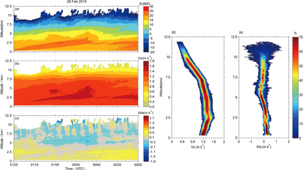
The Z and Vr values detected during selected snowfalls on 27, 28, 29 January, 28 February, 24 November 2015, as well as on 20 January 2016, are presented in Fig. 2. In order to exhibit the relatively complete evolution of snow clouds, the selected durations in the figure are slightly longer than those recorded by the ground snow observations. Among the six events, the clouds were mainly located below 8 km on 27, 28, 29 January 2015 and 20 January 2016 (Figs. 2a–d), whereas the echo tops reached 12 km or more in the other events (Figs. 2e, f). Small erect turrets appeared at the edges of the cloud where the GCs occurred, with different distribution densities. The Vr value changed rapidly in the GCs, and both updrafts and downdrafts were alternately observed. There were fibrous regions of large Z below the GCs, with Z-values generally greater than 10 dBZ. These were FSs, corresponding to a high Vr value above 1 m s−1. The values of Z and Vr for the FSs showed a trend of gradual enhancement with decreasing height. FSs may be influenced by horizontal wind moving out of the beam or merging as the height decreases. It has been indicated in previous studies (e.g., Plummer et al. 2014; Keeler et al. 2016b) that the existence of GCs is almost ubiquitous during snowfall, serving as an initial nucleation and growth mechanism for ice crystals.

The six snow events revealed that there are two types of location heights for GCs and two patterns of their associated FSs. The first type is represented by the events of 27, 28, 29 January 2015 and 20 January 2016 (Figs. 2a–d). In these events, the GCs were located at the tops of relatively shallow clouds. The GC heights were consistently about 5 km in the events of 27 January 2015, and 20 January 2016. During the events of 28 and 29 January 2015, the GC heights fluctuated, ranging primarily from 5 km to 7 km. The vertical extent of the GCs was relatively small, approximately 0.5–1.5 km. The Z-value rapidly increased from about −20 to around 0 dBZ, and Vr fluctuated mainly between −1 and 1 m s−1 within the GCs. The GC distribution was sometimes quite dense, and fibrous FSs were traced from the GCs that were densely distributed. FSs with high Z generated by falling ice crystals gradually combined into bands as they got closer to the ground, and they became relatively uniform before reaching the ground.
The second type of snow event is represented by the snowfall events of 28 February 2015 and 24 November 2015 (Figs. 2e, f). GCs were located at the tops of deep clouds, and the heights of the GC tops were above 10 km. The vertical extent of the GCs was relatively large, mainly around 2 km, and an increase in Z took place over a greater distance within the GCs. The cloud structure was relatively uniform in height, whereas the fluctuations of Vr within GCs were similar to those in the first type of snow event. The key similarity among the six events was that Z-values greater than 20 dBZ were only found below 5 km. The average T value at 5 km was about −15°C.
3. Analysis of the atmospheric environment
3.1 Synoptic background
Reanalysis data from the European Centre for Medium-Range Weather Forecasts were used to analyze the weather conditions, with a resolution of 0.25° × 0.25°. The event of 20 January 2016, was selected to represent the first event type, and the event of 28 February 2015, was selected to represent the second event type.
For the event of 20 January 2016, the weather conditions at 1200 UTC were analyzed. We mainly focused on the wind, temperature, and specific humidity fields at 700 hPa, as well as the wind, height, and temperature fields at 850 hPa. As can be seen in Figs. 3a and 3b, Shou County was located ahead of a southwest low-level jet, in advance of a trough at 700 hPa. This low-level jet was a very important water vapor transport channel, providing a source of water vapor for snowfall. The county was also located in the upward motion area southeast of the shear line of horizontal wind speed. Corresponding to the southwest jet at 700 hPa, an inverted trough could be observed at 850 hPa. The county was also near the top of the inverted trough, which was also the convergence zone formed by northerly and easterly airflow, leading to an area of upward air motion.

As can be seen from the 500 hPa plot in Fig. 4a, corresponding to the event of 28 February 2015, at 0000 UTC, the temperature trough to the north of Shou County lagged behind the height trough. The cold advection following the trough was favorable for the trough's development. The county was still located ahead of the southwesterly jet, as shown in Fig. 4b, where the warm, wet, southwesterly jet converged with the dry, cold, northwesterly airflow. The significant wind shear above Shou County made the airflow converge and rise. The frontal system tilted to the northwest with height, and Shou County lay behind the surface cold front. During this snow process, cold air in middle to high latitudes advected southward and influenced the county. The system was deeper than that of the event of 20 January 2016.
3.2 Vertical stratification
Owing to the lack of sounding data in Shou County, atmospheric stratification was analyzed at the Fuyang meteorological station using Skew-T diagrams and profiles of relative humidity (RH) with respect to water and supersaturation with respect to ice (Si). The same events as in Section 3.1 were selected for analysis, as shown in Fig. 5.
The RH was directly obtained by air sounding data. The detected RH can be transformed into RH with respect to ice (RHi) using WMO formulations about calculating the saturation vapor pressure over a surface of ice and liquid water below 0°C (World Meteorological Organization 2008).
The saturation vapor pressure over liquid water below 0°C (ew) was calculated using the following Eq.:
with
T in °C and
ew in hPa.
The saturation vapor pressure over ice (ei) was calculated using the following Eq.:
with
T in °C and
ei in hPa.
The actual vapor pressure (e) was obtained by multiplying ew by RH (e = ew RH), and RHi was obtained by dividing e by ei (RHi = e/ei). The value of Si (Si = RHi − 100 %) was also calculated.
In Figs. 5a and 5b, the thermal profiles showed that, below 1,000 hPa, all values of T were lower than 0°C. Thus, snowflakes did not undergo any melting or phase transformation while falling. There was a T inversion layer between 850 and 700 hPa, and the T-dew point difference was very small, indicating that stratiform clouds with increasing T and humidity existed in this layer.
As shown in Fig. 5a (deep event on 28 Feb 2015), the T–dew point difference below 300 hPa was very small, corresponding to large RH values shown in Fig. 5c. Si values below 13 km were greater than 0, indicating that the entire region was saturated with respect to ice. The Si value reached a maximum of 40 % at 12 km, where the echo top was located.
As shown in Fig. 5b (shallow event on 20 Jan 2016), the dew point profile above the saturated layer sloped steeply toward low T, resulting in a sharp decrease in ambient humidity and the formation of a dry layer. Thus, there was no cloud above ∼ 6 km, corresponding to the similar height of echo top seen in Fig. 2d. There was a near-saturated thin layer above the dry layer located near 300 hPa. However, perhaps because of its short duration and thin thickness, the cloud echo was not observed at the corresponding height. The region above the dry layer had no effect on the snowfall process, which was ignored in the following analysis.
In Fig. 5d, similar to the analysis results of the Skew-T diagram, the RH values remained above 90 % under 4 km and then decreased slightly with height until they sharply decreased to ∼ 20 % above 6 km. The Si values were greater than 0 between 1 and 6 km, indicating that the region inside the cloud was saturated with respect to ice. Ignoring the region above the dry layer, Si reached a maximum of 40 % near 6 km, where the echo top was located.
4. Analysis of the vertical structure
In this section, six typical time periods marked by red double arrows in Fig. 2 were selected for specific analyses at first, and then the partition method for the GC and St regions was determined. Finally, the characteristics of the GC regions in the six events were analyzed.
4.1 Properties of the vertical structure
a. Vertical structure
Contoured frequency by altitude diagrams (CFADs; Yuter and Houze 1995) of Z, Vr, and the gradients of Z (dZ/dh) and Vr (dVr/dh) are shown in Fig. 6 (four shallow events) and Fig. 7 (two deep events) to study the properties of vertical evolution. In order to prevent noise near the echo top from interfering with the analysis, following the method of estimating the cloud top altitude described by Plummer et al. (2014), the threshold of Vr variance was again adopted as 0.8 m2 s−2. However, according to the sensitivity of the CVPR-FMCW near 6 km and 12 km (the height of the echo top for the two types of snow events), the threshold of Z was changed to −28 dBZ and −22 dBZ, respectively. As the data reliability of the first four range gates was not high, the CFADs began with the fifth range gate (150 m).

The dZ/dh and dVr/dh values between every two adjacent range gates (30 m) were obtained to bolster the understanding of vertical variation about Z and Vr. The dZ/dh and dVr/dh were vertical gradients in the downward direction calculated with respect to the direction toward the ground. Positive values of dZ/dh and dVr/dh indicate that Z and Vr increase with decreasing height, whereas negative values imply the opposite.
As height decreased, the Z-values initially increased and then decreased slightly in the six snow events. The maximum Z-values (Zmax) were approximately 25 dBZ near 2.5 km above the ground. The Z-values were usually between 10 and 20 dBZ when snowflakes reached the ground. Compared with the distribution range of Z, that of Vr was relatively concentrated, mainly from 0 to 2 m s−1. Negative Vr appeared in the upper regions of the clouds, indicating the existence of upward air motion.
In Figs. 6 and 7, within 1–2 km below the cloud top, the distribution range of dZ/dh and dVr/dh widened. The distribution width of dVr/dh reached ∼ 1 m s−1, which was significantly higher than that in the rest of the cloud (mainly within 0.4 m s−1). The fluctuation of dVr/dh indicated that Vr changed rapidly, perhaps influenced by air motion. Within ∼ 1 km above the ground, the Z-values showed a decreasing trend, possibly because of the effect of decreasing humidity, as shown in Fig. 5.
b. Differences of shallow and deep events
Figure 6 illustrates that the Z-values increased quickest in regions approximately 1–2 km below the cloud top, and the maximum values of dZ/dh were encountered at these depths. As for shallow events, the maximum values reached 2 dB/30 m, even above 5 dB/30 m. Deeper in these regions, the growth rate of the Z-values became slower. The range of dVr/dh was also largest in those same regions. The ranges of dZ/dh and dVr/dh values were relatively narrow beneath the regions near the cloud top, indicating that the lower regions were relatively uniform and stable.
The CFADs shown in Fig. 7 correspond to the two deep events. The Z-values increased a little faster in the regions around 2 km beneath the cloud top compared to the regions below. The range of dZ/dh values in the regions near the cloud top was narrower than that of the shallow events, indicating that the rate and amplitude of the variation of the Z-values were relatively small in the deep events. The differences in dZ/dh between the regions near the cloud top and the rest were also smaller compared to the shallow events. The range of dVr/dh values in the upper regions was similar to that of the shallow events, whereas that of the dZ/dh values was a little narrower in the deep events. Note that because of the limitation of radar sensitivity, some weak signals may not be captured near the top of the deep events, so the calculated dZ/dh may be smaller than the actual values.
4.2 Characteristics analysis
The characteristics of Z and Vr in regions near the cloud top were similar to those of the GC regions described in the literature (e.g., Plummer et al. 2014; Rosenow et al. 2014). As shown in Figs. 2, 6, and 7, the uniformity and character of the echoes are distinct between the GC regions near the cloud top and the rest of the clouds, termed St regions. The two regions could be divided by the differences in dZ/dh and dVr/dh.
After analyzing the full datasets, it was determined that dZ/dh > 0.6 dB/30 m and |dVr/dh| > 0.08 m s−1/30 m could be used as GC indicators for the shallow events, whereas dZ/dh > 0.2 dB/30 m and |dVr/dh| > 0.08 m s−1/30 m could be used as GC indicators for the deep events. If the three continuous range gates designated as x1, x2, and x3 did not simultaneously meet the indicator criteria, the corresponding height of x1 (the range gate at the top of the three) was considered to be the height of the bottom of the GC. Note that the differences between the GC and St regions are gradual, so it is hard to determine a clear boundary. The partition method presented here extracts regions with obvious GC features from a statistical perspective and regards the rest as relatively stable St regions. The purpose is to quantitatively describe the characteristics of GC regions for further analyses. The black lines in Fig. 2 represent the boundaries between the two regions obtained using this method, and the periods with obvious GC features account for about 90 % of all the periods during the six events.
The characteristics of the GC regions in the six events are shown in Table 3 (the statistics only refer to the snow periods recorded by ground observations), including the maximum times of GC appearance within 1 h, the depth, the ranges of T and RHi, the average proportions with respect to the whole cloud depth, and the average contribution of the GC region to the growth of the Z-value. Among these, the depth is obtained by subtracting the height of the bottom of the GC from the calculated cloud top height. The average proportion with respect to the whole cloud depth is the average ratio of the GC region depth to the whole cloud depth. The difference of Z-values (ΔZ) between the cloud top height and the height of the bottom of the GC is defined as ΔZ within the GC region, and the difference between the Z-value at the cloud top and Zmax is defined as the total ΔZ in the cloud. The average ratio of ΔZ within the GC region to the total ΔZ is defined as the average contribution of the GC region to the growth of the Z-value. The depths of the GC regions are in good accord with previous studies (e.g., Plummer et al. 2014; Rosenow et al. 2014).

These statistics indicate that, for shallow events, the T measurements at the height of GCs were mainly around −20°C. GC regions typically have a depth of 500–1,200 m, with ΔZ mainly distributed between 23 and 27 dB. The depths of the GC regions accounted for about 11–14 % of the whole cloud. As for shallow events, the average contributions of the GC regions reached 42 %. GCs appeared up to 23 times within 1 h, resulting in dense fibrous FSs below.
There were some differences in the statistical characteristics between the two types of snow events. For the deep events, the depths of the GC regions were greater, reaching over 2 km. The times of GC appearance within 1 h were about one-third to one-half those in the shallow events, leading to the relatively sparse FSs and uniform St regions below. The T measurements at the height of the GCs were low, mainly distributed around −50°C. Because of the high altitude, the RH values were also lower than those found in the shallow events, but the RHi values at the height of the GCs were greater than 120 % for all six events, indicating that the environment was supersaturated with respect to ice. The depths of the GC regions accounted for about 16 % of the whole cloud, whereas the average contributions to the growth of the Z-values reached 33 % in these regions. Many previous studies also showed that the majority of ice growth typically occurred below the GC level (e.g., Matejka et al. 1980; Houze et al. 1981; Plummer et al. 2015), whereas the contributions of the GC regions to Z-value growth were larger than those to ice mass growth described in the above articles. Overall, the results revealed that, in the deep events, the proportions of the GC regions were slightly larger, but the average contributions to the growth of the Z-values were lower than those in the shallow events.
During the shallow events, because of the higher temperatures in the GC regions, supercooled water may still exist (Plummer et al. 2014). Thus, ice particles may grow through deposition and riming. It has been reported in previous studies (e.g., Connolly et al. 2012) that the aggregation efficiency is relatively high between −20°C and −10°C and reaches its maximum at −15°C. Ice particles in the GC regions may also grow rapidly by aggregation.
During the deep events, the GC regions featured low T and water vapor content and it was not possible for riming to exist without supercooled water (T < −40°C), which led to the relatively slow growth of ice particles. However, the GC region was located at great heights with low T and high RHi, an environment conducive to the deposition nucleation of ice crystals (Welti et al. 2014), which might contribute to the increase in particle number concentration. The ice particles in the GC regions may feature a high number concentration and slow growth rate, whereas Z is more sensitive to changes in the particle size. Therefore, we considered that, in the GC regions of deep events, the Z-values may not increase as fast as they do in the GC regions of shallow events, so the calculation error of dZ/dh may not be significant. We will provide evidence for this inference in our next article on microphysical properties.
According to the apparent differences between the surrounding regions and the inside of GCs and FSs exhibited in time–height contours of Z, the dZ/dh values between the inside and outside of the GCs and FSs were presumed to be different. In order to facilitate statistical analyses, the definition of the inside of a GC as presented by Plummer et al. (2014) was accepted, and we also used the threshold of 4 dB relative maxima in the Z time series measurements. In order to identify FSs, the method described by Plummer et al. (2015) was followed and the 45 s window was adopted. As the FSs were tilted, the calculation of dZ/dh within FSs was additionally explained here. The calculation of dZ/dh inside FSs was based on the measurements classified as FSs at each height. We believed that particles affected by the same horizontal wind moved at the same speed in the horizontal direction, so the earliest falling particles also reached the same lower height firstly. Between two adjacent range gates, the dZ/dh values inside FSs were obtained by Z-values classified as FSs at a lower range gate minus those at an adjacent higher range gate successively (i.e., the first Z-value classified as an FS at a lower range gate minus that at an adjacent higher range gate, etc.). The statistical results are summarized in Table 4.

As illustrated in Table 4, between the two types of events, the differences of the average dZ/dh in the GC regions were significant, whereas the differences in the St regions were relatively small. In the shallow events, the differences of the average dZ/dh between the two regions were greater than those in the deep events. The two types of events also had similarities: the average dZ/dh values were usually two to three times (average: 2.6) larger inside the GCs compared to outside, and the differences between the inside and outside of the FSs were of similar magnitude.
5. Analysis of dynamical properties
5.1 Retrieval of dynamical properties
Vertical air motion is an important process in cloud dynamics and is crucial for the formation and maintenance of GCs (e.g., Heymsfield 1975; Hogan et al. 2002; Lothon et al. 2005). It is necessary to acquire Wa values in clouds to analyze the dynamical processes during the nucleation and growth of particles. The retrieval method of Wa is introduced below.
a. Algorithm
The Vr value measured using a vertically pointing radar is the sum of Vz and Wa (Matrosov et al. 2002). According to Rogers (1964), in order to obtain Wa, the relationship between Z and Vz first needs to be established, followed by estimating Vz via the Z-value measured by the radar, correcting this estimation with air density, and finally calculating Wa by subtracting the corrected Vz value from Vr. There are two main methods for acquiring the Z–Vz relationship using a single radar. The first uses particle size distribution and the relationship between Vz and particle size (D) to deduce the Z–Vz relationship (e.g., Rogers 1964; Hauser and Amayenc 1981; Ulbrich and Chilson 1994), whereas the second consists of separating Vz and Wa by means of statistical methods along with the addition of some hypothetical conditions (e.g., Orr and Kropfli 1999; Matrosov et al. 2002; Protat et al. 2003; Plana-Fattori et al. 2010). The Z–Vz relationship for liquid particles has previously been expressed clearly (e.g., Marks and Houze 1987; Black et al. 1996; Joss and Waldvogel 1970), whereas the Vz value of solid particles is related to their habit and density, which increases the complexity of obtaining the Z–Vz relationship.
As mentioned in Section 2.1, the CVPR-FMCW can output precise power spectra of the return signal. As the minimum detection capability of the CVPR-FMCW can reach up to −170 dBm, the weak signals returned by small particles can be captured. As small particles at upper levels fall slowly, basically moving with the air motion, they can be regarded as tracers of the mean vertical air motion (e.g., Gossard et al. 1997; Babb et al. 1999; Kollias et al. 2001). When the vertical air motion is upward, these small particles are driven to move upward, forming low spectral peaks in the negative-velocity region (downward Vr values are positive) of the Doppler velocity spectra. The upward small particles in the negative-velocity region and the falling particles in the positive-velocity region form a distinctly bimodal spectrum. When the vertical air motion is downward, bimodal spectra sometimes occur, depending upon the breadth of the particle size distribution. In previous studies (e.g., Shupe et al. 2008; Zheng et al. 2017), identification and separation of bimodal Doppler velocity spectra were often used to extract Wa in clouds. In our study, Wa and Vz were retrieved and the Z–Vz relationship was established using spectral data with distinctly bimodal distributions.
Figures 8a and 8c present the typical detection results of the bimodal spectra in the GC and St regions, respectively, during the event of 20 January 2016. Figure 8b was selected from the single modal spectra region between the two bimodal spectra regions. In order to clearly show the bimodal phenomenon, the ordinates in the figures are represented by normalized power and all Doppler spectra are smoothed using a three-point boxcar averaging window. Moreover, the heights of the spectra are marked in the figures. By inspecting the spectra, it was seen that the first peak in the GC region occurred in the positive-velocity range, whereas the other occurred in the negative-velocity range, as seen in Fig. 8a. In the St region, both peaks were primarily in the positive-velocity range, as seen in Fig. 8c.

In the GC region, the spectral peak first appeared at negative (ascending) velocities, and it also appeared at positive velocities with the reduction of height. Initially, the right spectral peak was small and the left peak was dominant. As the height decreased, the right spectral peak increased rapidly, eventually exceeding the left one, which gradually weakened and disappeared. The left peak was associated with small particles, which could be interpreted as reflecting the vertical air motion. As the particles grew, those with fall speeds greater than the updraft velocities began to descend, leading to the formation of the spectral peak at positive velocities (the peak corresponds to large particles, hereinafter referred to as the LP peak). As the height decreased, the sizes and masses of the particles gradually increased, leaving fewer small particles. This might explain the gradual disappearance of the left spectral peak and the dominance of the right peak. This result is consistent with the study of Shupe et al. (2004).
The spectral peak for Wa in the St region appeared near 0 m s−1 and was always located to the left of the LP peak. The Wa peak became slightly enhanced with decreasing height, but it was always weaker than the LP peak. Weaker peaks mostly appeared near −8°C to −3°C. It has also been shown in some relevant studies (e.g., Zawadzki et al. 2001; Oue et al. 2018) that bimodal spectra in snow were often observed near −8°C to −3°C, which corresponds to secondary ice generation via the Hallett-Mossop process (Hallett and Mossop 1974), indicating the existence of supercooled droplets as well. Typical cloud droplets with a negligible terminal fall speed (Vt) were regarded in many studies as tracers of vertical air motion (e.g., Shupe et al. 2004, 2008). However, the Z-value of the weaker spectral peak in the St region was sometimes caused by cloud droplets and the small ice crystals produced by secondary ice generation, rather than just by cloud droplets. In this case, the velocity corresponding to the weaker peak was the sum of the downward air velocity and Vt of small secondary ice crystals, leading to a uncertainty in the estimation of Wa and Vz. The error estimation is discussed in Section 5.1.b.
As there are evident differences between the main spectral characteristics of the GC and St regions, in order to retrieve Wa and Vz more accurately, the Wa and LP peaks in the bimodal spectra of the two regions were identified, respectively, according to the spectral peak-picking algorithm described by Shupe et al. (2004). Note that the criteria were adjusted because the cases, radar wavelengths, and sampling parameters were different in our study. The criteria for picking secondary peaks were adjusted to at least two standard deviations (SDs) of noise greater than the spectral noise level (original threshold: 2.5). Additionally, the width of the spectral peaks was adjusted to at least 0.4475 m s−1 (or four continuous velocity bins) above the noise level (the original threshold was seven continuous velocity bins).
When a Wa peak was identified in a given Doppler spectrum, the Wa value was then estimated by the offset of the spectral peak from 0 m s−1. The influence of Wa was then removed from the detected Vr to obtain a more accurate Vz value. Using the calculated Vz (in m s−1) and the corresponding Z-values (in mm6 m−3), the Z–Vz power-law relationship with the generic form of Vz = aZb can be established by fitting (note that the Vz values were referenced to the ground level). The data points obtained using the bimodal spectra in the GC regions of shallow and deep events are shown in Figs. 9a and 9b, respectively. Equations (3) and (4) depict the relationships that were established for the GC regions in the shallow and deep events, respectively (the subscripts “s” and “d” represent shallow and deep events, respectively, and the subscript “1” represents the GC region), represented by the blue solid lines in Figs. 9a and 9b:

The quality of fit for Eq. (3) was indicated by an R2 value of 0.9172, with a root mean square error (RMSE) of 0.093, which represented a reasonably good fit. As for Eq. (4), the R2 value was 0.9025 and the RMSE was 0.090.
The data points obtained from the bimodal spectra in the St regions of shallow and deep events are shown in Figs. 9c and 9d, respectively. The Z-values of those weaker peaks were below −20 dBZ. In order to reduce the retrieval error, the data obtained from weaker peaks with a Z-value lower than −25 dBZ were selected to establish the Z–Vz relationship. Equations (5) and (6) depict the relationships for the St regions in the shallow and deep events, respectively (the subscript “2” represents the St region), represented by the blue solid lines in Figs. 9c and 9d:
The quality of fit for Eq. (5) was indicated by an R2 value of 0.9128, with an RMSE of 0.091. As for Eq. (6), the R2 value was 0.8986 and the RMSE was 0.089.
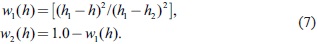
Orr and Kropfli (1999) reported that a single power-law equation cannot be used to produce the profiles of Vz throughout the depth of a cloud. There was usually a height range without double peaks between the two regions with bimodal spectra. In order to capture the continuous changes of Wa and Vz in the whole cloud, the height-weighted algorithm presented by Heymsfield et al. (2010) was used to calculate Wa and Vz for the region without bimodal spectra. The corresponding height at the top of the region was designated as h1, whereas that at the bottom of the region was designated as h2. At a certain height (h) between h1 and h2, the weights for Eqs. (3) and (4) and for Eqs. (5) and (6) are, respectively, given by the following Eq.:
The value of Vz in this region can be derived using the following Eq.:
where
Vz (
h),
Vz1 (
h), and
Vz2 (
h) are
Vz,
Vz1, and
Vz2 at height
h, respectively.
The Z-values measured by the CVPR-FMCW during the six snow events in our study were substituted into Eqs. (3)–(6) to calculate the value of Vz of the solid particles. Following correction for air density, the Wa value in the GC and St regions can be retrieved using the following equations:
where
h is the height;
Wa (
h),
Vr (
h), and
Vz (
h) are
Wa,
Vr, and
Vz at height
h, respectively; the subscripts “1” and “2” represent the GC region and the St region, respectively;
ρ0 is the air density at the ground, and
ρ(
h) is the air density at height
h. Additionally, the
Wa value in regions without bimodal spectra can be retrieved using the following Eq.:
b. Test of the retrieval results
Equations (3)–(6) were compared with the Z–Vz relationships of other solid particles with different habits. Hong (2007) introduced five particle habit assumptions: hexagonal columns (COL), bullet rosettes (ROS), aggregates (AGG), hexagonal plates (PLA), and droxtals (DRO). Protat and Williams (2011) deduced five relationships for the above five particle habits using the maximum particle dimension of Heymsfield and Iaquinta (2000) and the radar backscattering coefficients of Hong (2007) to calculate the radar backscattering cross section from the assumed ice particle size distribution. They also found that using these five habits was sufficient to represent the natural variability of solid particles. The a and b coefficients of the Z–Vz relationships corresponding to COL, PLA, and ROS were a = 0.65, b = 0.10; a = 0.44, b = 0.09; and a = 0.52, b = 0.10, respectively. The comparison results among Eqs. (3) and (4) and the three relationships for COL, PLA, and ROS are shown in Figs. 9a and 9b. As can be seen in the figure, Eq. (3) was closest to the relationship corresponding to PLA and Eq. (4) was closest to the relationship corresponding to ROS. These results indicated that PLA might be the predominant particle type in the GC region of shallow events, whereas ROS might be the predominant particle type in the GC region of deep events. The inferences about particle habits are consistent with the observations made by Plummer et al. (2014).
The a and b coefficients of the Z–Vz relationship corresponding to rimed AGG were a = 0.78 and b = 0.11 (Protat and Williams 2011). The a and b coefficients of the Z–Vz relationship corresponding to unrimed snow were a = 0.817 and b = 0.063 (Heymsfield et al. 2010). The comparison results among Eqs. (5) and (6) and the two relationships for AGG and snow are shown in Figs. 9c and 9d. As can be seen in the figure, the calculated Vz values from Eq. (5) basically fall between the Vz values from the other two equations of AGG and snow. In cases with the same Z-value, the maximum difference between Eq. (5) and the other two equations was nearly 0.1 m s−1. The comparison result of Eq. (6) was similar to that of Eq. (5), but the Vz value calculated using Eq. (6) was slightly larger for the same Z-value. This result indicated that either unrimed snow or rimed AGG might be the predominant particle type in the St region.
As described in Section 5.1.a, using the Z–Vz relationships to estimate Wa and Vz in the St regions may produce errors, and the errors are caused by the Vt of small secondary ice crystals.
Mossop (1976) reported that, on average, one ice splinter is thrown off for every 250 droplets (diameter ≥ 24 µm) accreted. As droplets smaller than approximately 13 µm are also necessary for the Hallett–Mossop process (Mossop 1978), it is assumed that the average diameter of the droplets in the cloud is 20 µm with a backscattering cross section of about 1.99 × 10⁻¹⁵ mm2. It has been shown in many studies that secondary ice crystals are mainly needle and columnar crystals (e.g., Heymsfield and Willis 2014; Oue et al. 2018) with a mean particle size of 120 µm (Zawadzki et al. 2001). For example, for a long columnar ice crystal, the backscattering cross section is about 9.77 × 10⁻¹⁴ mm2, as calculated using the discrete dipole approximation (DDA) method. The number concentration ratio of cloud droplets to ice crystals is supposed to be 250:1, so the Z-ratio is calculated to be 5.1:1. The maximum Z-value of the selected weaker spectral peak is −25 dBZ, and the Z-value of small ice crystals is estimated according to the Z-ratio. Using the Z-value of small ice crystals, the backscattering cross section calculated using the DDA method, the assumed ice particle size distribution (Hong 2007), and the relationship between Vt and the maximum particle dimension for columns (Heymsfield and Iaquinta 2000), it can be estimated that the Vt value of secondary columns is about 0.16 m s−1. As the Z-values of selected weaker peaks in the St regions were below −25 dBZ, it was estimated that 0.16 m s−1 is the maximum error caused by ignoring the Vt value of small secondary particles.
When the Vt value of small ice crystals is not considered, the downward air velocity in the lower part of the St region with bimodal spectra may be overestimated, resulting in the underestimation of Vz. In the upper part of the St region without bimodal spectra, the underestimated Vz value calculated using the Z–Vz relationship would lead to the underestimation of the absolute value of upward air velocity (negative value).
The dynamical properties of the two cloud regions are analyzed in the following sections. Two typical events and time periods are selected to represent the shallow and deep events, respectively.
5.2 Case study
a. Shallow event
Figure 10 shows the time-height contours of Z, Wa, and Vz and CFADs (Yuter and Houze 1995) of Wa and Vz during the period from 1230–1330 UTC of the event of 20 January 2016 (beginning with the fifth range gate). As shown in Figs. 10b and 10d, Vz evidently accelerated within the GCs, with speeds rapidly increasing from 0.2 to over 0.6 m s−1. The Vz in the St region, which was mainly over 0.8 m s−1, was faster than that found in the GC region. The proportion for the velocity range of 0.8–1 m s−1 was the largest, reaching more than 30 %. As the height decreased, the proportion increased. FSs with enhanced Z-values are shown clearly in Fig. 10a. The Vz value within FSs was higher than that between them, with a rate above 1 m s−1.

As shown in Figs. 10c and 10e, the GC locations usually correlated with strong upward air motion, having speeds of up to 1.5 m s−1, whereas downward air motion often appeared in the regions between GCs. Convective activities were obvious in the GC region. The high Z-values in the GC regions usually correspond to the large values of Vz and upward air motion. Upward motion plays a crucial role in cold clouds, as they affect the supply rate of water vapor and the activation rate of ice nuclei (Lin et al. 1998). Stronger upward motion causes more water vapor and activates more ice nuclei. Hence, more ice crystals are formed by nucleation with faster growth, leading to higher Z-values. Meanwhile, upward motion increases the probability of collisions among particles, which might promote the aggregation growth of particles and contribute to the increase of Z-values. For shallow events, the RH obtained by air sounding was usually close to or even more than 100 % in the GC regions, so there could also be a possibility of riming.
The upper part of the St region (∼ 3.5–4.5 km) contained mainly upward motion, with speeds ranging between 0.2 and 0.6 m s−1, corresponding to the magnitude of synoptic-scale rising motion, as analyzed in Section 3.1. Below ∼ 3.5 km, weak downward air motion dominated, with speeds slower than 0.5 m s−1. There was no apparent difference in Wa inside and outside the FSs, which is consistent with the finding of Plummer et al. (2015).
b. Deep event
Figure 11 shows the time-height contours of Z, Wa, and Vz and the CFADs of Wa and Vz during the period from 0020–0120 UTC of the event of 28 February 2015 (beginning with the fifth range gate). The distribution characteristics of Wa and Vz in this event were similar to those in the shallow event. In order to avoid repeating the above description, the following discussion focused on the differences between the two types of events.
In the GC region, the maximum velocity of the downdraft was slower than that during the shallow event. In the St region, Vz increased from 0.7 to 1.6 m s−1, with a velocity range of 1.2–1.4 m s−1 accounting for the largest proportion, over 40 %. The upper part of the St region featured weak upward air motion (∼ 5–8 km), with speeds ranging between 0.2 and 0.6 m s−1, also corresponding to the magnitude of synoptic-scale rising motion, as analyzed in Section 3.1. Weak downward air motion dominated the region below 5 km, with speeds slower than 0.5 m s−1.
In the St regions, there were few double peaks in the weak updraft layers (i.e., upper parts of the St regions). The vertical air velocities in these layers were obtained by subtracting Vz, calculated from the Z–Vz relationships, from the observed Vr. Radar observations showed that the Vr values in the upper updraft layers were smaller than those in the lower downdraft layers; therefore, the upward air velocities (negative values) occurred in the upper parts of the St regions after retrieval. The values of Z and calculated Vz in the upper updraft layers were also smaller, so the negative air velocities were mainly caused by the observed slow Vr. Therefore, we believe that the existence of updraft layers was reasonable.
5.3 Characteristics analysis
In this section, all six events were statistically analyzed to discuss the similarities and differences in the characteristics of Wa and Vz in two regions of the two event types and to compare the differences between the inside and outside of the GCs along with FSs. The statistical characteristics of Wa are summarized in Table 5. As there was no apparent difference in Wa inside and outside the FSs, while the upper and lower parts of the St regions seemed to feature different Wa values, the statistics on the averages and SDs of Wa in the upper and lower parts of the St regions replaced the statistics on those inside and outside the FSs. Negative values represented upward motion.

In the GC regions, the distribution range of Wa was mainly between −1.6 m s−1 and 1.5 m s−1 for the two types of events, which is similar to what was found in previous studies (e.g., Rosenow et al. 2014; Rauber et al. 2015). The upward air velocities within the GCs for the two types of events were similar, and the average speeds were mostly distributed around 1.2 m s−1. There were a few differences in the downward air velocities between the GCs for the two types of events, and the average speeds were mostly distributed around 1 m s−1. The SDs inside the GCs were larger than outside, with an average value of about 0.3 m s−1, whereas the SDs outside the GCs were about 0.25 m s−1 on average, indicating that the distribution of Wa inside the GCs was more discrete than outside. No evident differences in the SDs existed between the two types of events.
In the St regions, the distribution ranges of Wa were similar for the two types of events, mainly in the range of ±0.4 m s−1. The vertical air motion was much weaker in the St regions compared to the GC regions. The upper parts of the St regions consisted primarily of weak upward motion, with average speeds mostly distributed around 0.3 m s−1, which is consistent with previous studies (e.g., Rauber et al. 2014b; Plummer et al. 2015), whereas weak downward motion dominated the lower parts, with average speeds mostly distributed around 0.2 m s−1. The SDs of Wa were smaller in the St regions compared to the GC regions, indicating that the distribution of Wa in the St regions was more concentrated. The SDs of Wa were similar in the upper and lower parts of the St regions during the two types of events.
The statistical characteristics of Vz are summarized in Table 6. In order to guarantee a good retrieval accuracy, the minimal effective value for the Vz retrieval result was set to 0.2 m s−1. In the GC regions, the average speeds inside the GCs were around 0.6 m s−1, whereas those outside the GCs were around 0.4 m s−1, with differences ranging between 0.1 m s−1 and 0.3 m s−1. The SDs inside the GCs were larger than outside, indicating that the distribution of Vz inside the GCs was more discrete than outside. The SDs inside and outside the GCs were slightly larger during the shallow events compared to the deep events, indicating that the distribution of Vz in the shallow events was more discrete.

In the St regions, the Vz values were generally larger compared to the GC regions, mainly distributed above 0.8 m s−1. The average speeds inside the FSs were around 1.3 m s−1, whereas those outside the FSs were around 1 m s−1, with differences ranging between 0.2 m s−1 and 0.4 m s−1. As reported by Locatelli and Hobbs (1974), the fall speeds of solid particles are related to the maximum dimensions, mass, density, habits, and degree of riming of particles. The specific causes of the enhanced Vz within the GCs and FSs will be further analyzed in the next article on microphysical properties. At present, it can be concluded that the enhanced Vz within the GCs and FSs implies that more conducive conditions for particle growth exist in the GCs and FSs. The characteristics of the SDs were similar to those in the GC regions, with larger SDs inside the FSs and in shallow events.
6. Conclusions
Continuous observation data of six snow events were obtained using a CVPR-FMCW system that has an extremely high resolution during the winter of 2015–2016 in the midlatitudes of China. GCs described in previous research were found near the cloud tops in every event. Four out of the six events were shallow processes, with the echo top mainly below 8 km. The other two events were deep processes, with the echo top mostly above 10 km. The vertical fine structure and dynamical properties inside the two types of snow clouds were analyzed. The main conclusions of this study can be summarized as follows:
-
(1) According to the characteristics of echo distribution and the changes of dZ/dh and dVr/dh, snow clouds can be divided into GC regions and St regions. For shallow events, statistical analyses of the GC regions indicated that they typically have a depth of 500–1200 m. The depths of the GC regions accounted for about 11–14 % of the whole clouds, whereas the average contributions to the growth of Z-values reached 42 % in these regions. GCs occurred up to 23 times within 1 h, resulting in dense fibrous FSs below. As for deep events, the depths of the GC regions were greater, reaching over 2 km. The times of GC appearance within 1 h were about one-third to one-half those in the shallow events, leading to relatively sparse FSs and uniform St regions below. The depths of the GC regions accounted for about 16 % of the whole clouds, whereas the average contributions to the growth of Z-values reached 33 % in these regions. The contributions of the GC regions to Z-value growth were larger than those to ice mass growth described in some previous studies (e.g., Matejka et al. 1980; Houze et al. 1981; Plummer et al. 2015). In deep events, the proportions of GC regions were slightly larger, but the average contributions to the growth of Z-values were lower than those in shallow events. The depths of the GC regions are in good accord with previous studies (e.g., Plummer et al. 2014; Rosenow et al. 2014).
-
(2) Between the two types of events, the differences of the average dZ/dh in the GC regions were significant, whereas the differences in the St regions were relatively small. In the shallow events, the differences of the average dZ/dh between the two regions were greater than those in the deep events. The two types of events also had similarities: the average dZ/dh values were usually two to three times (average: 2.6) larger inside the GCs compared to outside, and the differences between the inside and outside of the FSs were of similar magnitude.
-
(3) Both updrafts and downdrafts were alternately observed in the GC regions. The distribution range of Wa was mainly between −1.6 m s−1 and 1.5 m s−1 for the two types of events, which is similar to what was found in previous studies (e.g., Rosenow et al. 2014; Rauber et al. 2015). GC locations usually correlated with strong upward air motion, whereas downward air motion often appeared in the regions between GCs. The air velocities in the GC region for the two types of events were similar, with average velocities mostly distributed around −1.2 m s−1 and 1 m s−1, respectively. The SDs of Wa inside the GCs were larger than outside, indicating that the distribution of Wa inside the GCs was more discrete than outside. No evident difference in the SDs of Wa existed between the two types of events. In the St regions, the speeds of Wa were mainly within 0.5 m s−1. There was no apparent difference in Wa inside and outside the FSs, which is consistent with the findings of Plummer et al. (2015). The upper parts of the St regions consisted primarily of weak upward motion, which is in good accord with previous studies (e.g., Rauber et al. 2014b; Plummer et al. 2015), whereas weak downward motion dominated the lower parts. The SDs of Wa were smaller in the St regions compared to the GC regions, indicating that the distribution of Wa in the St regions was more concentrated. The SDs of Wa were similar in the upper and lower parts of the St regions during the two types of events.
-
(4) In the GC regions, the SDs of Vz inside the GCs were larger than outside, indicating that the distribution of Vz inside the GCs was more discrete than outside. The SDs of Vz inside and outside the GCs were slightly larger during the shallow events compared to the deep events, indicating that the distribution of Vz in the shallow events was more discrete. In the St regions, the characteristics of the SDs of Vz were similar to those in the GC regions, with larger SDs of Vz inside FSs and in shallow events. The average speeds were slightly faster inside the GCs and FSs compared to outside, with differences of 0.1–0.3 m s−1 and 0.2–0.4 m s−1, respectively. The enhanced Vz value within the GCs and FSs implied that more conducive conditions for particle growth existed in GCs and FSs.
Using the Z–Vz relationships to estimate Wa and Vz in the St regions may produce errors, and 0.16 m s−1 is the maximum error caused by ignoring the Vt value of small secondary ice crystals related to the weaker spectral peaks.
The results of this study have, therefore, clarified the findings of the past half-century. The Wa and Vz values were retrieved more precisely using bimodal spectra from CVPR-FMCW. Moreover, the characteristics of the GC regions, as well as the average reflectivity gradients and dynamical properties inside and outside the GCs and FSs, were quantified. The results of this research may improve the understanding of the differences between the inside and outside of the GCs and FSs during the two types of snow events in terms of vertical reflectivity gradients and dynamical properties. The vertical structure and continuous evolution of Wa and Vz in snow clouds were also presented more clearly. The microphysical properties and physical mechanisms of the snow processes induced by GCs will be further analyzed using in situ observation data and simulation models based on this study.
Acknowledgment
This work has been supported by the National Key Research and Development Program of China under Grant 2017YFC1501703, National Natural Science Foundation of China (41675029, 41975046), research project of State Key Laboratory of Severe Weather. We would like to thank LetPub (www.letpub.com) for providing linguistic assistance during the preparation of this manuscript. The assistance of Jisong Sun (a researcher at State Key Laboratory of Severe Weather, Chinese Academy of Meteorological Sciences) in analyzing the environmental background is greatly appreciated.
References
- American Meteorological Society, 2016: Generating cell. Glossary of meteorology. [Available at http://glossary.ametsoc.org/wiki/Generating_cell.]
- Atlas, D., R. C. Srivastava, and R. S. Sekhon, 1973: Doppler radar characteristics of precipitation at vertical incidence. Rev. Geophys., 11, 1-35.
- Babb, D. M., J. Verlinde, and B. A. Albrecht, 1999: Retrieval of cloud microphysical parameters from 94-GHz radar Doppler power spectra. J. Atmos. Oceanic Technol., 16, 489-503.
- Bergeron, T., 1950: Über der mechanismum der ausgeibigen Niederschläge. Ber. Dtsch. Wetterdienstes, 12, 225-232.
- Black, M. L., R. W. Burpee, and F. D. Marks, Jr., 1996: Vertical motion characteristics of tropical cyclones determined with airborne Doppler radial velocities. J. Atmos. Sci., 53, 1887-1909.
- Connolly, P. J., C. Emersic, and P. R. Field, 2012: A laboratory investigation into the aggregation efficiency of small ice crystals. Atmos. Chem. Phys., 12, 2055-2076.
- Cronce, M., R. M. Rauber, K. R. Knupp, B. F. Jewett, J. T. Walters, and D. Phillips, 2007: Vertical motions in precipitation bands in three winter cyclones. J. Appl. Meteor. Climatol., 46, 1523-1543.
- Crosier, J., T. W. Choularton, C. D. Westbrook, A. M. Blyth, K. N. Bower, P. J. Connolly, C. Dearden, M. W. Gallagher, Z. Cui, and J. C. Nicol, 2014: Microphysical properties of cold frontal rainbands. Quart. J. Roy. Meteor. Soc., 140, 1257-1268.
- Cunningham, J. G., and S. E. Yuter, 2014: Instability characteristics of radar-derived mesoscale organization modes within cool-season precipitation near Portland, Oregon. Mon. Wea. Rev., 142, 1738-1757.
- Douglas, R. H., K. L. S. Gunn, and J. S. Marshall, 1957: Pattern in the vertical of snow generation. J. Meteor., 14, 95-114.
- Gossard, E. E., J. B. Snider, E. E. Clothiaux, B. Martner, J. S. Gibson, R. A. Kropfli, and A. S. Frisch, 1997: The potential of 8-mm radars for remotely sensing cloud drop size distributions. J. Atmos. Oceanic Technol., 14, 76-87.
- Gunn, K. L. S., M. P. Langleben, A. S. Dennis, and B. A. Power, 1954: Radar evidence of a generating level for snow. J. Meteor., 11, 20-26.
- Hallett, J., and S. C. Mossop, 1974: Production of secondary ice particles during the riming process. Nature, 249, 26-28.
- Hauser, D., and P. Amayenc, 1981: A new method for deducing hydrometeor-size distributions and vertical air motions from Doppler radar measurements at vertical incidence. J. Appl. Meteor., 20, 547-555.
- Heymsfield, A., 1975: Cirrus uncinus generating cells and the evolution of cirriform clouds. Part II: The structure and circulations of the cirrus uncinus generating head. J. Atmos. Sci., 32, 809-819.
- Heymsfield, A. J., and J. Iaquinta, 2000: Cirrus crystal terminal velocities. J. Atmos. Sci., 57, 916-938.
- Heymsfield, A., and P. Willis, 2014: Cloud conditions favoring secondary ice particle production in tropical maritime convection. J. Atmos. Sci., 71, 4500-4526.
- Heymsfield, G. M., L. Tian, A. J. Heymsfield, L. Li, and S. Guimond, 2010: Characteristics of deep tropical and subtropical convection from nadir-viewing high-altitude airborne Doppler radar. J. Atmos. Sci., 67, 285-308.
- Hogan, R. J., P. R. Field, A. J. Illingworth, R. J. Cotton, and T. W. Choularton, 2002: Properties of embedded convection in warm-frontal mixed-phase cloud from aircraft and polarimetric radar. Quart. J. Roy. Meteor. Soc., 128, 451-476.
- Hong, G., 2007: Radar backscattering properties of non-spherical ice crystals at 94 GHz. J. Geophys. Res., 112, D22203-, doi:10.1029/2007JD008839.
- Houze, R. A., Jr., S. A. Rutledge, T. J. Matejka, and P. V. Hobbs, 1981: The mesoscale and microscale structure and organization of clouds and precipitation in mid-latitude cyclones. III: Air motions and precipitation growth in a warm-frontal rainband. J. Atmos. Sci., 38, 639-649.
- Ikeda, K., R. M. Rasmussen, W. D. Hall, and G. Thompson, 2007: Observations of freezing drizzle in extratropical cyclonic storms during IMPROVE-2. J. Atmos. Sci., 64, 3016-3043.
- Joss, J., and A. Waldvogel, 1970: Raindrop size distributions and Doppler velocities. Preprints, 14th Conference on Radar Meteorology. Tucson, AZ, Amer. Meteor. Soc., 153-156.
- Keeler, J. M., B. F. Jewett, R. M. Rauber, G. M. McFarquhar, R. M. Rasmussen, L. Xue, C. Liu, and G. Thompson, 2016a: Dynamics of cloud-top generating cells in winter cyclones. Part I: Idealized simulations in the context of field observations. J. Atmos. Sci., 73, 1507-1527.
- Keeler, J. M., B. F. Jewett, R. M. Rauber, G. M. McFarquhar, R. M. Rasmussen, L. Xue, C. Liu, and G. Thompson, 2016b: Dynamics of cloud-top generating cells in winter cyclones. Part II: Radiative and instability forcing. J. Atmos. Sci., 73, 1529-1553.
- Keeler, J. M., R. M. Rauber, B. F. Jewett, G. M. McFarquhar, R. M. Rasmussen, L. Xue, C. Liu, and G. Thompson, 2017: Dynamics of cloud-top generating cells in winter cyclones. Part III: Shear and convective organization. J. Atmos. Sci., 74, 2879-2897.
- Keppas, S. C., J. Crosier, T. W. Choularton, and K. N. Bower, 2018: Microphysical properties and radar polarimetric features within a warm front. Mon. Wea. Rev., 146, 2003-2022.
- Kollias, P., B. A. Albrecht, R. Lhermitte, and A. Savtchenko, 2001: Radar observations of updrafts, downdrafts, and turbulence in fair-weather cumuli. J. Atmos. Sci., 58, 1750-1766.
- Kumjian, M. R., and K. A. Lombardo, 2017: Insights into the evolving microphysical and kinematic structure of northeastern U.S. winter storms from dual-polarization Doppler radar. Mon. Wea. Rev., 145, 1033-1061.
- Kumjian, M. R., S. A. Rutledge, R. M. Rasmussen, P. C. Kennedy, and M. Dixon, 2014: High-resolution polarimetric radar observations of snow-generating cells. J. Appl. Meteor. Climatol., 53, 1636-1658.
- Langille, R. C., and R. S. Thain, 1951: Some quantitative measurements of three-centimeter radar echoes from falling snow. Can. J. Phys., 29, 482-490.
- Langleben, M. P., 1956: The plan pattern of snow echoes at the generating level. J. Meteor., 13, 554-560.
- Li, N., Z. Wang, K. Sun, Z. Chu, L. Leng, and X. Lv, 2018: A quality control method of ground-based weather radar data based on statistics. IEEE Trans. Geosci. Remote Sens., 56, 2211-2219.
- Lin, H., K. J. Noone, J. Ström, and A. J. Heymsfield, 1998: Small ice crystals in cirrus clouds: A model study and comparison with in situ observations. J. Atmos. Sci., 55, 1928-1939.
- Locatelli, J. D., and P. V. Hobbs, 1974: Fall speeds and masses of solid precipitation particles. J. Geophys. Res., 79, 2185-2197.
- Lothon, M., D. H. Lenschow, D. Leon, and G. Vali, 2005: Turbulence measurements in marine statocumlus with airborne Doppler radar. Quart. J. Roy. Mereor. Soc., 131, 2063-2080.
- Marks, F. D.,Jr., and R. A. Houze, Jr., 1987: Inner core structure of Hurricane Alicia from airborne Doppler radar observations. J. Atmos. Sci., 44, 1296-1317.
- Marshall, J. S., 1953: Precipitation trajectories and patterns. J. Atmos. Sci., 10, 25-29.
- Marshall, J. S., and K. L. S. Gunn, 1952: Measurement of snow parameters by radar. J. Meteor., 9, 322-327.
- Matejka, T. J., R. A. Houze, Jr., and P. V. Hobbs, 1980: Microphysics and dynamics of clouds associated with mesoscale rainbands in extratropical cyclones. Quart. J. Roy. Meteor. Soc., 106, 29-56.
- Matrosov, S. Y., A. V. Korolev, and A. J. Heymsfield, 2002: Profiling cloud ice mass and particle characteristic size from Doppler radar measurements. J. Atmos. Oceanic Technol., 19, 1003-1018.
- Mossop, S. C., 1976: Production of secondary ice particles during growth of graupel by riming. Quart. J. Roy. Meteor. Soc., 102, 45-57.
- Mossop, S. C., 1978: The influence of drop size distribution on the production of secondary ice particles during graupel growth. Quart. J. Roy. Meteor. Soc., 104, 323-330.
- Orr, B. W., and R. A. Kropfli, 1999: A method for estimating particle fall velocities from vertically pointing Doppler radar. J. Atmos. Oceanic Technol., 16, 29-37.
- Oue, M., P. Kollias, A. Ryzhkov, and E. P. Luke, 2018: Toward exploring the synergy between cloud radar polarimetry and Doppler spectral analysis in deep cold precipitating systems in the Arctic. J. Geophys. Res., 123, 2797-2815.
- Pfitzenmaier, L., Y. Dufournet, C. M. H. Unal, and H. W. J. Russchenberg, 2017: Retrieving fall streaks within cloud systems using Doppler radar. J. Atmos. Oceanic Technol., 34, 905-920.
- Plana-Fattori, A., A. Protat, and J. Delanoe, 2010: Observing ice clouds with a Doppler cloud radar. C. R. Phys., 11, 96-103.
- Plummer, D. M., G. M. McFarquhar, R. M. Rauber, B. F. Jewett, and D. C. Leon, 2014: Structure and statistical analysis of the microphysical properties of generating cells in the comma head region of continental winter cyclones. J. Atmos. Sci., 71, 4181-4203.
- Plummer, D. M., G. M. McFarquhar, R. M. Rauber, B. F. Jewett, and D. C. Leon, 2015: Microphysical properties of convectively generated fall streaks within the stratiform comma head region of continental winter cyclones. J. Atmos. Sci., 72, 2465-2483.
- Protat, A., and C. R. Williams, 2011: The accuracy of radar estimates of ice terminal fall speed from vertically pointing Doppler radar measurements. J. Appl. Meteor. Climatol., 50, 2120-2138.
- Protat, A., Y. Lemaitre, and D. Bouniol, 2003: Terminal fall velocity and the FASTEX cyclones. Quart. J. Roy. Meteor. Soc., 129, 1513-1535.
- Rauber, R. M., M. K. Macomber, D. M. Plummer, A. A. Rosenow, G. M. McFarquhar, B. F. Jewett, D. Leon, and J. M. Keeler, 2014a: Finescale radar and airmass structure of the comma head of a continental winter cyclone: The role of three airstreams. Mon. Wea. Rev., 142, 4207-4229.
- Rauber, R. M., J. Wegman, D. M. Plummer, A. A. Rosenow, M. Peterson, G. M. McFarquhar, B. F. Jewett, D. Leon, P. S. Market, K. R. Knupp, J. M. Keeler, and S. M. Battaglia, 2014b: Stability and charging characteristics of the comma head region of continental winter cyclones. J. Atmos. Sci., 71, 1559-1582.
- Rauber, R. M., D. M. Plummer, M. K. Macomber, A. A. Rosenow, G. M. McFarquhar, B. F. Jewett, D. Leon, N. Owens, and J. M. Keeler, 2015: The role of cloud-top generating cells and boundary layer circulations in the finescale radar structure of a winter cyclone over the Great Lakes. Mon. Wea. Rev., 143, 2291-2318.
- Rauber, R. M., S. M. Ellis, J. Vivekanandan, J. Stith, W.-C. Lee, G. M. McFarquhar, B. F. Jewett, and A. Janiszeski, 2017: Finescale structures of a snowstorm over the northeastern United States: A first look at high-resolution HIAPER Cloud Radar observations. Bull. Amer. Meteor. Soc., 98, 253-269.
- Rogers, R. R., 1964: An extension of the Z-R relation for Doppler radars. Proceedings of The 11th Weather Radar Conference. Boston, MA, Amer. Meteor. Soc., 158-161.
- Rosenow, A. A., D. M. Plummer, R. M. Rauber, G. M. McFarquhar, B. F. Jewett, and D. Leon, 2014: Vertical velocity and physical structure of generating cells and convection in the comma head region of continental winter cyclones. J. Atmos. Sci., 71, 1538-1558.
- Ruan, Z., L. Jin, R. S. Ge, F. Li, and J. Wu, 2015: The C-band FMCW pointing weather radar system and its observation experiment. Acta Meteor. Sin., 73, 577-592.
- Schultz, D. M., D. S. Arndt, D. J. Stensrud, and J. W. Hanna, 2004: Snowbands during the cold-air outbreak of 23 January 2003. Mon. Wea. Rev., 132, 827-842.
- Shupe, M. D., P. Kollias, S. Y. Matrosov, and T. L. Schneider, 2004: Deriving mixed-phase cloud properties from Doppler radar spectra. J. Atmos. Oceanic Technol., 21, 660-670.
- Shupe, M. D., P. Kollias, M. Poellot, and E. Eloranta, 2008: On deriving vertical air motions from cloud radar Doppler spectra. J. Atmos. Oceanic Technol., 25, 547-557.
- Syrett, W. J., B. A. Albrecht, and E. E. Clothiaux, 1995: Vertical cloud structure in a midlatitude cyclone from a 94-GHz radar. Mon. Wea. Rev., 123, 3393-3407.
- Takahashi, T., T. Endoh, G. Wakahama, and N. Fukuta, 1991: Vapor diffusional growth of free-falling snow crystals between −3 and −23°C. J. Meteor. Soc. Japan, 69, 15-30.
- Ulbrich, C. W., and P. B. Chilson, 1994: Effects of variations in precipitation size distribution and fallspeed law parameters on relations between mean Doppler fallspeed and reflectivity factor. J. Atmos. Oceanic Technol., 11, 1656-1663.
- Welti, A., Z. A. Kanji, F. Lüönd, O. Stetzer, and U. Lohmann, 2014: Exploring the mechanisms of ice nucleation on kaolinite: From deposition nucleation to condensation freezing. J. Atmos. Sci., 71, 16-36.
- Wen, M., S. Yang, A. Kumar, and P. Zhang, 2009: An analysis of the large-scale climate anomalies associated with the snowstorms affecting China in January 2008. Mon. Wea. Rev., 137, 1111-1131.
- Wexler, R., 1955: Radar analysis of precipitation streamers observed 25 February 1954. J. Meteor., 12, 391-393.
- World Meteorological Organization, 2008: Appendix 4B, Guide to meteorological instruments and methods of observation. WMO-No. 8 (CIMO Guide), Geneva.
- Yuter, S. E., and R. A. Houze, Jr., 1995: Three-dimensional kinematic and microphysical evolution of Florida cumulonimbus. Part II: Frequency distributions of vertical velocity, reflectivity, and differential reflectivity. Mon. Wea. Rev., 123, 1941-1963.
- Zawadzki, I., F. Fabry, and W. Szyrmer, 2001: Observations of supercooled water and secondary ice generation by a vertically pointing X-band Doppler radar. Atmos. Res., 59-60, 343-359.
- Zheng, J., L. Liu, K. Zhu, J. Wu, and B. Wang, 2017: A method for retrieving vertical air velocities in convective clouds over the Tibetan Plateau from TIPEX-III cloud radar Doppler spectra. Remote Sens., 9, 964, doi:10.3390/rs9090964.
- Zhou, W., J. C. L. Chan, W. Chen, J. Ling, J. G. Pinto, and Y. Shao, 2009: Synoptic-scale controls of persistent low temperature and icy weather over southern China in January 2008. Mon. Wea. Rev., 137, 3978-3991.