Articles
Intra-day Forecast of Ground Horizontal Irradiance Using Long Short-term Memory Network (LSTM)
2020 Volume 98 Issue 5 Pages 945-957

Details
2020 Volume 98 Issue 5 Pages 945-957
Accurate forecast of global horizontal irradiance (GHI) is one of the key issues for power grid managements with large penetration of solar energy. A challenge for solar forecasting is to forecast the solar irradiance with a lead time of 1–8 hours, here termed as intra-day forecast. This study investigated an algorithm using a long short-term memory (LSTM) model to predict the GHI in 1–8 hours. The LSTM model has been applied before for inter-day (> 24 hours) solar forecast but never for the intra-day forecast. Four years (2010–2013) of observations by the National Renewable Energy Laboratory (NREL) at Golden, Colorado were used to train the model. Observations in 2014 at the same site were used to test the model performance. According to the results, for a 1–4 hour lead time, the LSTM-based model can make predictions of GHIs with root-mean-square-errors (RMSE) ranging from 77 to 143 W m−2, and normalized RMSEs around 18.4–33.0 %. With five-minute inputs, the forecast skill of LSTM with respect to smart persistence model is 0.34–0.42, better than random forest forecast (0.27) and the numerical weather forecast (−0.40) made by the Weather Research and Forecasting (WRF) model. The performance levels off beyond 4-hour lead time. The model performs better in fall and winter than in spring and summer, and better under clear-sky conditions than under cloudy conditions. Using adjacent information from the reanalysis as extra inputs can further improve the forecast performance.
Solar photovoltaic (PV) energy is a major source of renewable energy. Over the past decade it has been increasingly integrated into the worldwide electricity grid. Electricity output by solar panels depends on solar irradiance reaching the horizontal surface, a.k.a. global horizontal irradiance (GHI). GHI includes three components: direct solar beam; diffusive solar radiation by atmosphere and clouds; and ground-reflected solar radiation (usually insignificant). The GHI is affected by several environmental factors such as solar irradiance at the top of the atmosphere, cloud fraction, aerosol loading, and relative humidity. As a result, the amount of electricity produced by a solar panel is subjected to fluctuations in such meteorological variables (Bae et al. 2017). This is distinctively different from traditional power generators that are stable over the entire operational period and insensitive to actual weather variations. The effect of such fluctuations becomes significant when PV power generation consists of 5 % of overall power used over a local grid and becomes critical when the PV penetration reaches 20 % (Matsura 2009). As a result, some traditional generators must be used as a backup (a.k.a. operating reserve) to stabilize the power grid. However, conventional power generation systems (including nuclear) all have their own “warm-up” time, ramp rate, and minimal possible load (International Energy Agency 2014). Therefore, improving the accuracy of solar irradiance forecasting can be critically important for efficient grid management with large penetration of solar energy.
Depending on the need for solar energy for different time horizons, different types of solar forecasting techniques can be used. For example, intra-hour forecasting (also known as nowcasting) refers to prediction of GHI from a few minutes up to one-hour. With an assumption that cloud property does not change and merely moves with the wind (Bosch and Kleissl 2013; Chow et al. 2015; Chu et al. 2015; Lorenz et al. 2014; Rana et al. 2016), prediction of GHI is usually done by simply extrapolating current wind and cloud information. Thus, only endogenous data are needed for such forecasting. For another example, inter-day forecasting refers to prediction of changes of GHI for one to several days ahead, and, for such a timescale, the evolution of weather system becomes the leading factor in determining the variations of solar irradiance. As a result, the most useful inter-day forecasts heavily rely on the numerical weather prediction (NWP) (e.g., Alessandrini et al. 2015; Mellit et al. 2014; Almeida et al. 2015). Between the above two ends of time horizon is the intra-day forecast, i.e., solar forecasting with a lead time of 1–8 hours. Many cloud systems can develop, mature, and dissipate within eight hours. The multiscale turbulence nature of cloud systems plays important roles within such timescale. State-of-the-art NWP models still have difficulties simulating such phenomena and, therefore, also have difficulty to well resolve the GHI variations within 8 hours (Cros et al. 2014).
The machine-learning approach recently emerges as a promising alternative to do the intra-day forecast since neither simple extrapolation technique nor pure physics-based NWP technique has proved to be fully successful for such type of forecast (Antonanzas et al. 2016; Nonnenmacher and Coimbra 2014; Miller et al. 2018). A number of algorithms have been used to forecast the GHI over this timescale. For example, David et al. (2018) compared the intra-day forecasting of deterministic GHI by three models: coupled autoregressive and dynamical system (CARDS); sequential neural network (NN); and more traditional recursive autoregressive and moving average (ARMA) model. Their results showed that the performance of the ARMA model is comparable to that of NN, but both of them outperform the CARDS.
Some studies have employed Long Short-Term Memory networks (LSTMs) to forecast photovoltaic (Gensler et al. 2016), total electron content (Sun et al. 2017), and day-ahead solar irradiance (Qing and Niu 2018). LSTM is a particular kind of recurrent neural network (RNN; refer to the appendix) introduced by Hochreiter and Schmidhuber (1997). Wang et al. (2018) and Fu et al. (2016) found that a LSTM network can achieve a better performance than the traditional time series prediction methods such as the ARMA and Support Vector Machine Regression. There has to date to the best of our knowledge been no use of LSTM for intra-day solar forecasting. Therefore, inspired by the success of the LSTM for the inter-day solar forecasting, this study aims at assessing the performance of a LSTM-based model for intra-day solar forecasting. The remainder of this paper is organized as follows. Section 2 describes the observational data used in this study, the structure of the LSTM model used in this study, and the validation metrics used for assessing the performance of the forecast. Section 3 presents the forecasting results and sensitivity tests regarding the choices of input features, temporal resolutions, and some configurations of the LSTM model. Section 4 compares the performance of the LSTM model with that of several other forecast methods. Conclusions and further discussion are given in Section 5.
Figure 1 sketched the structure of LSTM-based time series prediction scheme used in this study. Mathematical description of the LSTM model can be found in the appendix. The LSTM has a special neuron structure called memory cell that can capture short-term memory and keep it for a long time (Graves 2012), unlike normal multi-layer perceptron framework. Three gates control the information flow into and out of the memory cell: input gate; output gate; and keep gate (also known as forget gate). If the forecast is made at time t0 using m sets of observations prior to it, m LSTM models are then needed. The features (i.e., inputs) fed into each LSTM model through the input gate can be GHI only (i.e., one feature only), as well as a set of features including GHI. For our case, the set of features include GHI, local time, and other observable meteorological variables including relative humidity (RH; %), total cloud fraction (Fcld ; unitless), near-surface temperature (Ts; K), and solar irradiance at the top of the atmosphere (Rtoa; W m−2), as shown in Fig. 1. These meteorological variables all have direct relevance to the solar radiative transfer in the atmosphere. All LSTM models were implemented using Keras neural network library (Chollet 2015), which runs on top of TensorFlow. Then used as the input to a dense layer to generate forecast of the GHI in the next n hours after time t0 is the output, which has a dimension of out_d, from the LSTM model. The final output for our case is hourly-averaged GHI for the n th hours after time t0. Previous studies such as those by Gensler et al. (2016) and Wang et al. (2018) showed that the input for such LSTM framework should be 2–5 times as long as the sequence of the forecast in order to do a sequence of forecast. Our targeted sequence is 8-hour GHI forecast, thus we have tested the length of input from 8 to 56 hours prior to the forecast time. It turns out that using 32-hour observations prior to the forecast time t0 has the optimal performance. In the following discussions, all results are obtained using 32 hours of features prior to the time of the forecast.
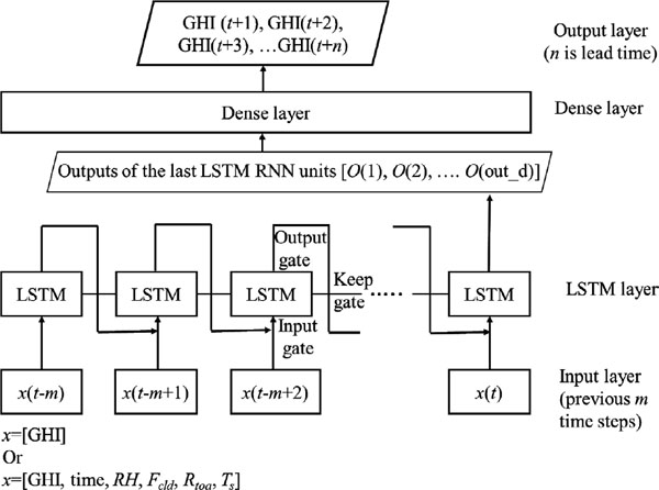
LSTM-based time series prediction framework. The input feature(s) is denoted as x and (m + 1) time steps in the past are used for input to predict m time steps in the future. Three gates control the information flow in and out of each LSTM cell, namely input gate, output gate, and keep gate.
The training was deemed finished when the RMSE decreases to a small value (in our case, ∼ 105 W m−2 or less) and keeps essentially flat within 50 more training iterations. Coefficients derived from such training were then saved and used to do the 8-hour forecast of GHI.
2.2 DataData used in this study was from ground observations at Golden, Colorado (39.74°N, 105.18°W, elevation of 1.829 km) by the National Renewable Energy Laboratory (NREL; Andreas and Stoffel 1981). Original observations were made every minute. Observed GHI, total cloud fraction, near-surface relative humidity, and temperature were used. The GHIs were measured using well-maintained global horizontal pyranometers with a 3–5 % measurement uncertainty (Wilcox 2012; Wilcox and Myers 2008). Four years of observations from 2010 to 2013 were used to train the LSTM network. The observations in the entire year of 2014 were then used for validation. The evaluation of the LSTM forecast performance with respect to different configurations of the network was also carried out using the same sets of training and validation data.
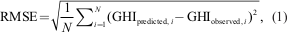
2.3 Metrics for evaluating the model performance: RMSE, nRMSE, and forecast skillMultiple metrics exist for evaluating the forecasting performance (Orwig et al. 2015). The most commonly used in meteorological forecast is root mean square error (RMSE), which is defined as:
 |
In addition, we will perform a linear fit of the predicted hourly GHIs with respect to the observed counterparts. The R-square from such linear fit tells the fraction of total variance in observed GHIs that can be explained by a linear function of predicted GHIs. Meanwhile, the slope of the linear fit tells the scaling of such linear function (with 1:1 being the ideal) and the intercept tells the bias of such linear fit.
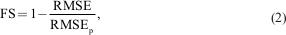
Forecast skill (FS), which is introduced by Coimbra et al. (2013), is widely used as a comparison metric in solar forecast. It is defined as:
 |
 |
 |
Firstly, 32 hours of high temporal resolution data (five minutes per data point) was used as input to the LSTM model with out_d = 100 to forecast GHIs in the next eight hours with also a temporal resolution of five minutes. In other words, 384 sequential inputs (i.e., 32-hour observations) were used to predict the next 96 sequential outputs (i.e., GHI forecast for the next eight hours). The input data vectors have six features including GHIs, time, total cloud fraction, relative humidity, near-surface temperature, and solar irradiance at the top of atmosphere (TOA). As the nighttime GHI is zero and has no relevance to solar power generation, only daytime forecast is examined further here.
Figure 2 shows the scatter plots between the predicated hourly-averaged GHIs and observed counterparts for a one-hour lead time (also referred to as one-hour forecast horizon). Results from four seasons are plotted separately. The largest deviation from 1:1 line is seen in spring, which has a slope of 1.09. All slopes are larger than 1 and, correspondingly, the intercepts are all negative, ranging from −2 W m−2 in winter to −20.5 W m−2 in spring. The R-squares range from 0.88 in the summer to 0.93 and 0.92 in the fall and winter seasons, respectively. Consistent with our understanding of the weather system, in general, the prediction performance is the best in winter and the poorest in summer. In winter, large-scale, long-lived weather systems affect the cloud evolutions the most. For example, when a synoptic frontal system passes the site, it usually is featured with overcast sky over a few days. Then the high-pressure system comes with entire clear-sky or little cloud coverage over a few days. In summer, however, diurnal cycle featured with local, short-lived convective storms dominates the cloud variations and thus the GHI is less predictable than in the winter and a large-scale weather system is less organized. This can also be seen from the scatter plots in Fig. 2: the linear model fit the wintertime data much better than the summertime data.
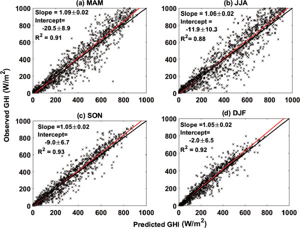
Scatter plot of the predicted verse observed hourly-averaged GHI. The prediction is for one-hour lead time. The entire year of 2014 data were used. Solid black lines are the 1:1 reference lines. Linear regression results are shown as red line. Each panel is for one season.
The RMSE, nRMSE, and linear regression outcomes (slope and intercept) for a lead time from one-hour to eight hours are summarized in Fig. 3. For annual average, the RMSE (nRMSE) increases from ∼ 77 W m−2 (∼ 18 %) at one-hour lead time to ∼ 143 W m−2 (∼ 33 %) at four-hour lead time. Both RMSE and nRMSE suggest that the forecast performance levels off beyond four hours. As expected, the winter-time RMSE is always the smallest among all seasons and for all lead times. Except for winter, the regression slopes (intercepts) for other seasons decrease (increase) with the increase of lead time, which can be explained by the fact that randomness increases with respect to the lead time (e.g., a convective storm or shower happens after forecast time t0 and lasts for only an hour or two), and such randomness has little dependence on what happens before t0. As explained above, winter weather is mostly governed by a largescale synoptic system that could last several days, which can account for the seasonal contrast here.
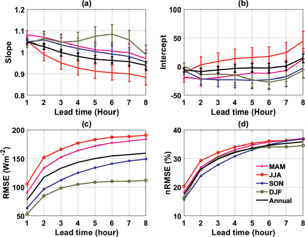
The LSTM performance for hourly-averaged GHI prediction with different lead time from one to eight hours. (a) regression slope; (b) intercept; (c) RMSE; and (d) nRMSE. Results from different seasons are shown in different colors. The performances for the entire year are shown in black curves.
The dependence of forecast performance with respect to cloud fraction is also examined. Figure 4 shows the performance metrics with respect to four groups of observed cloud fraction. The RMSE for the group with cloud fraction < 1 % is significantly less than those for the remaining three groups. The RMSE for such clear or nearly clear-sky situation mainly rises from the aerosol absorption and scattering of sunlight and the water vapor absorption of solar radiation. Due to measurement limitation, our input features do not include information about aerosols, while the input features such as surface temperature and relative humidity are related to water vapor. When cloud fraction is less than 95 %, the RMSE and nRMSE both level off after the 4th hour. However, this is not the case for overcast or nearly overcast situations, where both RMSE and nRMSE keep increasing with forecast horizon. The slope of regression also keeps dropping with increase of forecast horizon, dropping to as low as 0.6 for the 8th hour, but the intercept of regression is always less than 10 W m−2 and is nearly zero for the 8th hour. These highlight the challenge of solar forecasting for overcast skies. From the meteorological perspective, overcast sky implies small GHI and even a small amount of reduction in cloud fraction can quickly increase the amount of solar irradiance reaching the surface. Explaining at least partly why the forecast performance for this group is not as good as for the remaining three groups and why it has no apparent level off forecast horizon is that, within eight hours, an overcast sky at t0 can evolve to any possibilities (e.g., still overcast, completely clear-sky, and partly cloudy).
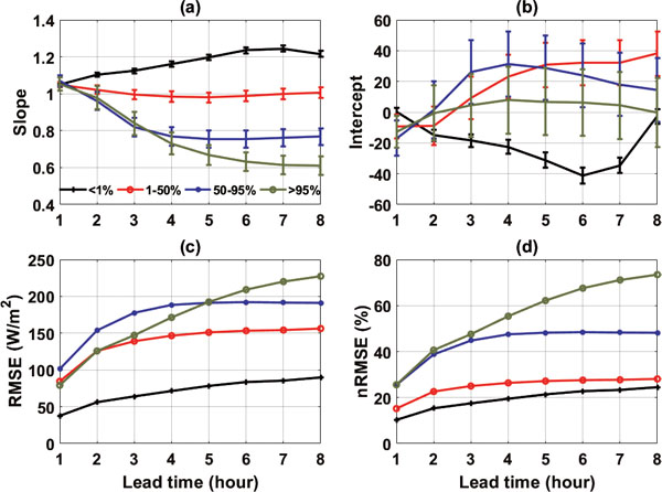
Performance of the LSTM forecast composite with respect to four groups of cloud fraction at forecast time zero: cloud fraction < 1 % in red; 1–50 % in red; 50–95 % in blue; and > 95 % in green. Four panels are the regression slope (a), regression intercept (b), RMSE (c) and nRMSE (d).
We further examine forecast performance with respect to the inputs at different temporal resolutions, to the different choices of input features, and to a key hyperparameter, the number of the last LSTM outputs (out_d). The goal is to estimate an optimal configuration for the LSTM forecast algorithm in terms of computational speed and accuracy. RMSE and nRMSE will be used in the assessment of different configurations, as they are more useful than the linear regression statistics for such purposes (Orwig et al. 2015).
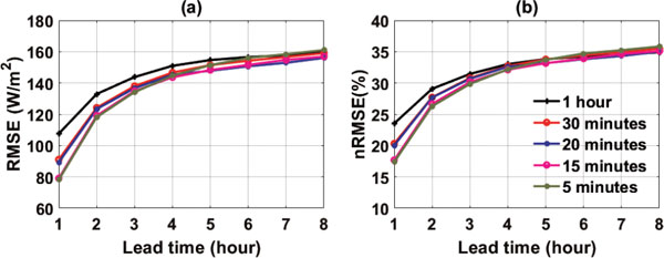
a. Temporal resolutionsFive temporal resolutions for the input features are tested, i.e., five-minute, 15-minute, 20-minute, 30-minute, and 1-hour inputs. Other configurations are identical to what is used in Section 3.1. For each temporal resolution, the LSTM network is trained separately. The performances are shown in Fig. 5. After the 4th hour, the RMSE and nRMSE both show little dependence on the temporal resolutions of the input features. Within four hours, a finer temporal resolution can improve the performance but the dependence is stepwise instead of linear. For example, the five-minute and 15-minute inputs have nearly identical performance, so do the 20-minute and half-hour inputs. The improvements from one-hour to half-hour resolution, in terms of RMSE and nRMSE, are ∼ 20 % while from half-hour to five-minute resolution the improvement is only ∼ 10 %. On the same computer platform, it takes 5, 22, 50, 88, and 790 seconds to finish one iteration of training for the inputs with 1-hour, 30-minute, 20-minute, 15-minute, and five-minute resolutions, respectively. The prediction takes 37, 134, 306, 480 and 4848 seconds for the inputs with 1-hour, 30-minute, 20-minute, 15-minute, and five-minute resolution, respectively. The computational cost from 15-minute to five-minute resolution increases by a factor of ∼ 10 while the forecast performance is comparable. Recommended among all temporal resolutions examined here are inputs with 15-minute resolution, given the RMSE dependence and the computing cost.
Among six input features, the most important one is observed GHI. It is meaningful to look a LSTM network using the GHI as the only input feature and to compare its performance with the counterpart that uses all six features as input to train the LSTM network. Figure 6 summarizes the comparisons of performance between six features and only the GHI feature. For the 1-hour inputs, though the 6-feature prediction always performs better than the one feature prediction, the difference is small for the first two hours (∼ 2 %) and then increases with the forecast horizon to ∼ 5 %. For the 15-minute inputs, the difference is only 1 % or less. On the same platform, one iteration in training of six-feature and one feature networks takes nearly the same amount of time. Given no difference in training, six features should be advocated instead of one feature. But if the data availability is an issue, GHI observation with high temporal resolution (15-minute or even higher) alone can be used for such forecast.
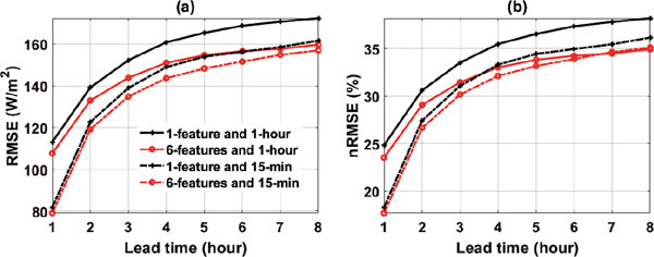
Sensitivity of RMSE (a) and nRMSE (b) to number of features used as the inputs. Results predicted using 1-hour inputs and 15-minute inputs are in solid and dashed lines, respectively. One feature is to use GHI only. Six features include time, GHI, total cloud fraction, solar irradiance at TOA, relative humidity, and air temperature. The same LSTM configuration used for Figs. 2–4 is used here.
Five configurations of out_d are tested. The performances are shown in Fig. 7. For 1-hour inputs (Figs. 7a, c), when out_d varies from 50 to 100, the performance is essentially the same. When out_d increases from 10 to 50, the performance is significantly improved for the first-hour prediction. For the case of 15-minute (Figs. 7b, d), however, changing out_d from 10 to 100 nearly leads to no improvement in the performance for all forecast horizons. The trade-off between out_d and the temporal resolution of the inputs can be clearly seen by contrasting left panels and right panels in Fig. 7. For a 1–5 hour lead time, the performances with any out_d using 15-minute inputs are better than the performances with out_d = 100 and 1-hour inputs. Beyond the 5th hour, however, the performance using 15-minute inputs becomes comparable to the performance using 1-hour inputs with out_d ≥ 50. The time to train a LSTM network with out_d = 100 is 2.5 times as much as the time needed to train a LSTM network with out_d = 10. Based on these facts, 15-minute inputs with out_d = 10 are an affordable option with performance no worse than any other configurations examined here.
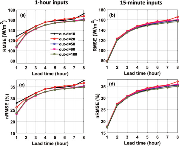
Sensitivity of RMSE and nRMSE to the number of LSTM output (out_d). Left column: 1-hour inputs are used. Right column: 15-minute inputs are used. Upper row is for RMSE and lower row is for nRMSE. Results from different out_ds are shown in different colors, as labeled in (a) for all the panels.
This section is to test whether the features from adjacent locations can help improve the forecast. Given that the actual GHI observations at neighboring locations to this NREL site are not available, we use hourly GHIs from the latest European Centre for Medium-Range Weather Forecasts (ECMWF) ERA5 reanalysis (Copernicus Climate Change Service 2017) over a 0.75-degree by 0.75-degree domain centered at the grid box encompassing NREL location. The hourly GHIs from ERA5 are at a resolution of 0.25-degree by 0.25-degree. The ERA5 GHIs on 3-by-3 grids are thus used as input features to the LSTM to predict the GHI at NREL, together with other features used in the previous subsections. Figure 8 shows the differences between with and without GHIs from the ERA5 reanalysis, for RMSE and nRMSE, respectively. The differences are negative up to a 7-hour lead time, with maximum difference being 5 W m−2 for the RMSE and 1 % for the nRMSE. Therefore, using neighboring GHI features near the observed site can help the prediction performance.
Using the FS defined in Subsection 2.3 as a metric, we compare the performance of LSTM with that of the random forest method (Breiman 2001) and of NWP made by the NCAR's Weather Research and Forecasting version 3.9 (WRF; Skamarock et al. 2008), as well as the FS from a physical method published by Miller et al. (2018). The same five-minute data used for the LSTM model training is used for the random forest training. The WRF model forecast domain is centered at NREL Golden site with an outside domain of 192 km by 192 km (a 3-km grid on each direction) nested with an inner domain of 64 km by 64 km (1-km grid on each direction). The model used NCEP operational Global Forecast System (GFS) analysis as initializations and lateral boundary conditions for a 8-hourly daytime forecast every day in 2015, and then the GHI forecast were evaluated against observation.
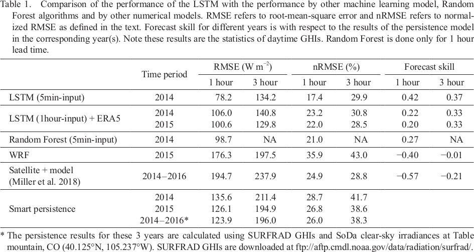
The overall comparisons are summarized in Table 1. The LSTM algorithm outperforms the random forest, with ∼ 2 % reduction for nRMSE and 8–10 W m−2 reduction in RMSE. Compared to numerical weather forecast by the WRF model, the LSTM algorithm can reduce RMSE by 54–68 W m−2 and nRMSE by ∼ 12 %. Miller et al. (2018) used a NWP model in combination with satellite-based cloud advection techniques to predict GHIs with a lead time of 1–3 hours. They evaluated their method at four different locations including the Table Mountain in Boulder, Colorado (40.125°N, 105.237°W), which is close to the NREL site. They found that, for this site over a three-year period, the 1-hour and 3-hour forecast RMSEs are 194.7 W m−2 and 237.9 W m−2, respectively. The FS is negative. These findings are comparable to our WRF model results (Table 1). In contrast, the 3-h and 1-h FSs of LSTM are 0.22–0.33 for hourly inputs and 0.37 ∼ 0.42 for 5-minute inputs, better than those of NWP forecast. FS for all 1–8 hour lead times is shown in Fig. 9. Overall, the FS in 2014 ranges from 0.22 to 0.39 for hourly inputs and from 0.34 to 0.42 for 5-minute inputs.
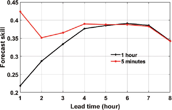
Forecast skill in 2014 compared to smart persistence model.
This study designed a LSTM-based model to perform intra-day GHI forecast and evaluated its performance using observations from a single station at Golden, Colorado by NREL. Four years of observations from 2010 to 2013 were used to train the model, and the evaluation is based on the prediction for the entire year of 2014. The normalized RMSE is ∼ 20 % for the 1st-hour prediction. Consistent with our physical understanding of the traits of different weather systems governing the GHI variations in different seasons, the performance is better in the winter (RMSE = 58.0 W m−2) than in the summer (RMSE = 109.1 W m−2). The forecast performance levels off after the fourth hour with a nRMSE around 30 %. The forecast skill to smart persistence model is 0.22–0.39 for hourly inputs and 0.34–0.42 for five-minute inputs. Such performance is better than that of forecast based on random forest method (0.27), and is much better than that of numerical weather forecast using the WRF model (−0.40). The performance within the first four hours shows dependence on the temporal resolution of the input features: inputs with high temporal resolution, in general, perform better than those with low temporal resolution but the performance shows stepwise dependence with temporal resolution. Using multiple features with physical relevance to GHI in the context of atmospheric radiation outperforms a single GHI feature, especially for forecast beyond two hours. But there is a trade-off between the temporal resolution of the inputs and the number of input features, as well as a trade-off between the temporal resolution of the inputs and the choice of a key hyperparameter, i.e., the number of outputs from the last cell of the LSTM (out_d). With computational cost and accuracy both considered, an optimal LSTM configuration for the intra-day GHI forecasting can be 15-minute GHI as the only input to LSTMs with out_d = 10. We also found that using the GHI features from neighbor locations (such as GHIs derived from the ERA5 reanalysis) can improve the LSTM model forecast performance.
This study explores the potential of LSTM in solar forecasting with the use of only indigenous observations. Limited by observational data, some key physical factors such as aerosol loadings were not available for this study. In principle, introducing such features that are directly related to GHI can have promise to further improve the performance of machine-learning based algorithm, which is one pathway that we are interested in pursuing further. Meanwhile, introducing features from other data sources, such as simultaneous satellite observations and information about largescale weather patterns from NOAA National Weather Service, also have a chance to improve the performance of such algorithms further. It is encouraging to further explore other RNNs in such forecast applications, if the LSTM, as one type of RNN, can be successfully employed for solar forecasting.
We want to thank two anonymous reviewers for their comments and suggestions. We also thank the Editorial Committee members for their comments and careful proofreads. The National Renewable Energy Laboratory (NREL) ground measurements are downloadable at https://midcdmz.nrel.gov/apps/go2url.pl? site=BMS. SoDa data is downloaded from http://www. soda-pro.com/web-services/radiation/cams-mcclear. GFS forecast and analysis data is downloaded from https://rda.ucar.edu/datasets/ds084.1/. The code used in this study is available at https://github.com/Huang-Group-UMICH/Solar_forecast_LSTM. This work was supported by Office of Research at the University of Michigan.
Details of LSTM neural network can be found in Olah (2015) and Sun et al. (2017). Below is a brief summary of the essence of LSTM. Figure A1 shows the typical LSTM neural network cell. The data flow in and out of three type of gates, namely h (t - 1) and x (t) as two input gates, C (t) as a keep gate, and h (t) as an output gate. h (t - 1) contains outputs from the previous LSTM cell state and x (t) are the current inputs directly from the input layer. C (t) and h (t) are expressed as:
 |
 |
 |
 |
 |
 |
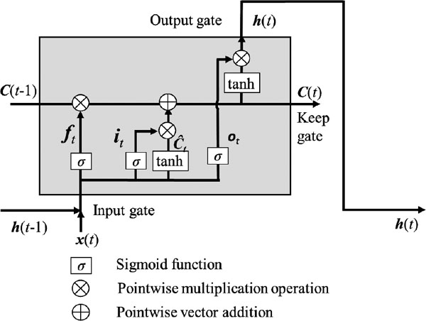
Sketch of the structure of LSTM neural network cell based on illustration from Olah (2015) and Sun et al. (2017).
Based on above formulas, the interpretation of each LSTM cell can be given as follow. ft is between 0 and 1, with one being completely keeping the previous cell state, C (t − 1), and zero being completely discarding it. Ĉt are new candidate values derived from tanh function with input of both outputs from the previous LSTM cell, h (t − 1), and the current input, x (t). it determines to what extent Ĉt is used for updating the current state C(t). ot decides the fraction of tanh (C(t)) to be used for computing the current output h(t).
