Assimilation of Lidar Water Vapour Mixing Ratio and Temperature Profiles into a Convection-Permitting Model

Abstract

The impact of assimilating thermodynamic profiles measured with lidars into the Weather Research and Forecasting (WRF)-Noah-Multiparameterization model system on a 2.5-km convection-permitting scale was investigated. We implemented a new forward operator for direct assimilation of the water vapor mixing ratio (WVMR). Data from two lidar systems of the University of Hohenheim were used: the water vapor differential absorption lidar (UHOH WVDIAL) and the temperature rotational Raman lidar (UHOH TRL). Six experiments were conducted with 1-hour assimilation cycles over a 10-hour period by applying a 3DVAR rapid update cycle (RUC): 1) no data assimilation 2) assimilation of conventional observations (control run), 3) lidar–temperature added, 4) lidar–moisture added with relative humidity (RH) operator, 5) same as 4) but with the WVMR operator, 6) both lidar–temperature and moisture profiles assimilated (impact run). The root-mean-square-error (RMSE) of the temperature with respect to the lidar observations was reduced from 1.1 K in the control run to 0.4 K in the lidar–temperature assimilation run. The RMSE of the WVMR with respect to the lidar observations was reduced from 0.87 g kg⁻¹ in the control run to 0.53 g kg⁻¹ in the lidar-moisture assimilation run with the WVMR operator, while no improvement was found with the RH operator; it was reduced further to 0.51 g kg⁻¹ in the impact run. However, the RMSE of the temperature in the impact run did not show further improvement. Compared to independent radiosonde measurements, the temperature assimilation showed a slight improvement of 0.71 K in the RMSE to 0.63 K, while there was no conclusive improvement in the moisture impact. The correlation between the temperature and WVMR variables in the static-background error-covariance matrix affected the improvement in the analysis of both fields simultaneously. In the future, we expect better results with a flow-dependent error covariance matrix. In any case, the initial attempt to develop an exclusive thermodynamic lidar operator gave promising results for assimilating humidity observations directly into the WRF data assimilation system.

1. Introduction

The vertical and horizontal distribution of water vapor and temperature in the atmosphere is crucial for the evolution of weather on all spatial and temporal scales. Detailed observations are important for improving the initial fields for numerical weather prediction (NWP) from nowcasting to the very short-range, the short-range, and the medium range. However, our present representation of land–atmosphere (L–A) interaction and convection initiation (CI) suffers in mesoscale models largely from huge observational gaps, consequently also limiting the predictive skill of NWP. Therefore, it is essential to enhance these observations and to investigate the impact of new remote sensing systems which are capable of measuring water vapor and temperature profiles into NWP models by means of data assimilation (DA).

Small-scale variations in moisture due to collision of boundaries (Kingsmill 1995), horizontal convective rolls and mesocyclones (Weckwerth et al. 1996; Murphey et al. 2006), and intersections between boundaries and horizontal convective rolls (Dailey and Fovell 1999) influences the location and timing of CI. The amount of moisture and variations in the vertical gradients of moisture and temperature at lower levels of the atmosphere can change the strength of CI significantly (Lee et al. 1991; Crook 1996). Several field campaigns have been conducted to understand the relationship between the three-dimensional thermodynamic fields and CI as well as the impact of assimilation of thermodynamic profiles. These have included the Mesoscale Alpine Program 1990 (Richard et al. 2007); the International H₂O Project (IHOP) 2002 (Weckwerth and Parsons 2006); the Convection Storm Initiation Project conducted in the summer period of 2004 and 2005 (Browning et al. 2007) and which provided sufficient data for impact studies using the Met Office unified model (Dixon et al. 2009); the Lindenberg Campaign for Assessment of Humidity and Cloud Profiling Systems and its Impact on High-Resolution Modeling (LAUNCH, Engelbart and Haas (2006) in the late summer of 2005; the Convective and Orographically-induced Precipitation Study (COPS) 2007 (Wulfmeyer et al. 2011); and the Plains Elevated Convection At Night (Geerts et al. 2017) campaign in summer 2015.

Recently, studies of land–atmosphere (L–A) feedback have also become the focus of improving the quality of weather forecast models as it was realized that a realistic representation of L–A interaction in mesoscale models is crucial for an accurate prediction of the pre-convective, dynamic, and thermodynamic environments. The first extensive study was the Land Atmosphere Feedback Experiment (Wulfmeyer et al. 2018) conducted in August 2017, which also provided a large data set for the assimilation of thermodynamic profiles measured with lidar in mesoscale models. The importance and sensitivity of L–A feedback for the simulation and prediction of the formation and organization of clouds and precipitation was exemplified in Santanello et al. (2018).

At the major forecast centers, there are mainly three DA approaches which are currently used: (1) variational techniques like 3DVAR and 4DVAR (Courtier 1998; Barker et al. 2004; Huang et al. 2009); (2) ensemble-based approaches which include flavors of the ensemble Kalman filter (Evensen 2003), and (3) hybrid combinations of these (Ingleby et al. 2013). In 3DVAR, the data is assimilated at specific analysis time-steps, whereas in 4DVAR there is an adjoint model so that the cost function is minimized over a time period and not at a particular time-step. The drawback of the 3DVAR is the static nature of the background error covariance (B) matrix in the cost function. This prevents the model from incorporating the present dynamics of the atmosphere. Although 4DVAR implicitly incorporates a time-evolving background error covariance model (Lorenc 2003), the same static matrix, B, is propagated implicitly to a later time-step. However, the 4DVAR is superior to the 3DVAR scheme due to the evolution of the background error covariance matrix and the reduction of the model imbalance at the analysis time. Meteo-France uses the incremental 3DVAR in the Aire Limitée Adaptation dynamique Développement Inter National (ALADIN) model (Brousseau et al. 2011; Berre 2000); the German Weather Service (DWD) and MeteoSwiss uses the Local Ensemble Transform Kalman Filter (LETKF) DA in the Consortium for Small-scale Modelling (COSMO) model (Schraff et al. 2016); the UK Met Office has implemented incremental 3DVAR and 4DVAR (Ingleby et al. 2013); NOAA's National Centers for Environmental Prediction uses incremental hybrid 3DEnVar and non-variational cloud analysis (Wu et al. 2017; Hu et al. 2006, 2017; Benjamin et al. 2004, 2016); and the Japan Meteorological Agency (JMA) applies incremental 4DVAR and 3DVAR (Honda et al. 2006; Aranami et al. 2015). A recent discussion of the DA methods used in various forecast centers is given by Gustafsson et al. (2018). All of these DA techniques are capable of assimilating profiles of the thermodynamics and dynamics of the atmosphere.

Radiosonde and aircraft measurements are the only conventional data observation sources currently providing water vapor and temperature data within the planetary boundary layer (PBL) and lower troposphere. Radiosondes provide a vertical thermodynamic profile of the atmosphere from the surface layer through the lower troposphere whereas weather stations provide only surface measurements with limited impact on the vertical thermodynamic structure. Radiosondes provide instantaneous data only at the time of ascent, giving more or less a snapshot of the atmosphere along their vertical track. Therefore, the soundings suffer from significant sampling errors, especially in the boundary layer with its highly turbulent fluctuations (Weckwerth et al. 1999). The coverage of the radiosonde network is quite coarse, and the number of radiosonde stations is decreasing rather than increasing in most countries due to their high cost of operation.

Another option is the application of passive and active remote sensing data. Wulfmeyer et al. (2015) gave a comprehensive overview of the current observational capabilities of remote sensing techniques with respect to thermodynamic fields in the lower troposphere. It was demonstrated that using space-borne passive remote sensing systems for thermodynamic observations does not provide the necessary vertical resolution in the lower troposphere to recover its vertical structure. Ground-based passive remote sensing instruments like microwave radiometers produce reliable data but have a coarse resolution of around 300 m to 1000 m in the lower 2000 m above the ground (Blumberg et al. 2015; Cadeddu et al. 2002; Wulfmeyer et al. 2015). IR spectrometers have higher vertical resolutions due to having more spectroscopic lines which can be evaluated; however, their vertical resolution is still limited to 100 m to 800 m up to 2000 m above ground level (Turner and Löhnert 2014). Convection-permitting models have vertical resolutions in the range of 100 m or less within the boundary layer, where fine-scale processes are crucial, in order to recover the thermodynamic structure of the atmosphere. Therefore the observation systems must fulfill the data requirements of convective-scale DA models to ensure higher representativeness (Wulfmeyer et al. 2015). Therefore, microwave radiometers and IR spectrometers are not capable of resolving the vertical structure of the lower troposphere, including the top of the PBL, the inversion strength at the PBL top, or the elevated inversion layers and the moisture structure in the free lower troposphere. However, this capability is expected to be crucial to achieving an improved prediction of L–A feedback and CI. Typical temporal resolutions of passive remote sensing instruments are 5–10 minutes, but further processing time is required either for the inversion of the spectra to vertical water vapor and temperature information or for the assimilation of the spectra through a forward operator in a DA system.

Active remote sensing techniques offer high temporal and spatial resolution data simultaneously to accurately capture the atmospheric fields without much loss of temperature and moisture gradient information. Two main techniques for humidity profiling are available: water vapor differential absorption lidar (WVDIAL) and water vapor Raman lidar (WVRL). Both systems achieve a high vertical and temporal resolution during both day- and night-time (Lange et al. 2018; Späth et al. 2018). Whereas WVDIAL does not require calibration (Ismail and Browell 1989; Bösenberg 1998), it has been demonstrated that, for WVRL, the calibration has long-term stability, and a high accuracy can be maintained for the measurements. Ground-based WVDIAL has been implemented for tropospheric measurements at various centers. Depending on the efficiency of the receiver and the average power of the laser transmitter, the combination of temporal and spatial resolution ranges from 1 s, 15 m (Metzendorf 2019) to 5 min, 300 m (Spuler et al. 2015). The NCAR and Montana State University have developed a compact, field-deployable micro-pulse DIAL (Spuler et al. 2015; Weckwerth et al. 2016) with a range resolution of 300 m and a temporal resolution of 1–5 min. The vertically pointing WVDIAL of the Institute of Physics and Meteorology (IPM, Wagner et al. 2011, 2013; Metzendorf 2019) has a range resolution of 15–300 m and temporal resolution of 1–10 s. The first WVDIAL with a 3-D scanner was also developed at the IPM of the University of Hohenheim (UHOH, Behrendt et al. 2009; Späth et al. 2014). Typical accuracies of the absolute humidity for the IPM's WVDIAL are in the range of 5–10 % within the PBL during the daytime. WVRLs have been making continuous measurements at various centers, such as the operational WVRL (Goldsmith et al. 1998; Turner and Goldsmith 1999) at the Atmospheric Radiation Measurements Southern Great Plains site in the U.S; the Raman Lidar for Meteorological Observations (RALMO, Dinoev et al. 2013; Brocard et al. 2013) in Payerne, Switzerland used by MeteoSwiss; the Raman Lidar for Atmospheric Moisture Sensing (RAMSES, Reichardt et al. 2012) in Lindenberg, Germany, used by the German Meteorological Service (DWD); and the WVRL at the Cabauw Experimental Site for Atmospheric Research (CESAR, Apituley et al. 2009) in the Netherlands. Typical resolutions of WVDIALs are around 150 m for the spatial resolution and 10 s for the temporal resolution, with an accuracy of < 5 %.

For temperature profiling in the lower troposphere, the temperature rotational Raman lidar (TRL) technique demonstrated the best performance (Behrendt et al. 2004; Di Girolamo et al. 2004; Arshinov et al. 2005; Radlach et al. 2008). It is now possible to measure temperature profiles from close to the surface to the lower troposphere with a temporal resolution of a few minutes and a vertical resolution of approximately 100 m. This performance permits the detection of inversion layers and the characterization of the temperature gradient with a high degree of accuracy (Hammann et al. 2015). Continuous time–height cross-sections of the atmospheric thermodynamic profile are a unique feature of these lidar systems which enables promising research and applications in the direction of mesoscale DA. Therefore, WVDIAL, WVRL, and TRL are suitable and ready for application in DA impact studies.

The subject of this work is the analysis of the impact of two relatively new lidar systems used for water vapor and temperature profiling in mesoscale DA. The two active remote sensing system are the high-power, high-efficiency, 3D scanning WVDIAL which has an extraordinary resolution, accuracy, and range (Wagner et al. 2013; Späth et al. 2014, 2016) and the TRL for daytime and night-time temperature profiling (Radlach et al. 2008; Hammann et al. 2015; Behrendt et al. 2015; Lange et al. 2018), both developed and operated at the IPM in Stuttgart, Germany.

The experimental setup was based on the Weather Research and Forecasting-Noah-Multiparameterization (WRF-Noah-MP) model system and the WRF DA (WRFDA) system using a 3DVAR rapid update cycle (RUC). This RUC was developed and optimized for Europe (Schwitalla and Wulfmeyer 2014) and is operated on the convection-permitting scale. Previously, the water vapor mixing ratio (WVMR) or other water vapor variables were assimilated by applying the radiosonde relative humidity (RH) operator. It is obvious that this is not the optimal approach because the RH is strongly sensitive to temperature. Therefore, we developed a new forward operator for the assimilation of absolute humidity, mixing ratio or specific humidity independent of any cross-sensitivity to temperature. This forward operator was based on an already-existing atmospheric infrared sounding retrieval (AIRSRET) observation operator in the WRFDA system. We expected that this new operator would provide a strong and direct impact. The first key objective of this work was to quantify this impact.

So far, there have been only a few impact studies using thermodynamic lidar data. During IHOP 2002, Wulfmeyer et al. (2006) assimilated airborne water vapor DIAL data from the NASA LASE system into the 5th generation Pennsylvania State University-NCAR Mesoscale Model (MM5), which was based on a 4DVAR DA system. The results from the assimilation resulted in a considerably improved prediction of CI due to strong and positive analysis increments, not only with respect to water vapor but also to dynamics. During LAUNCH, Grzeschik et al. (2008) assimilated water vapor data from a triangle of three WVRLs, again into the MM5. The initial water vapor field was corrected by about 1 g kg⁻¹ and the WVRL impact on the water vapor field continued for up to 12 h in the forecast model. Airborne water vapor data from the Water Vapour Lidar Experiment in Space demonstrator was assimilated into the ECMWF 4DVAR global model by Harnisch et al. (2011). The analysis error was reduced after the assimilation of WVDIAL observations. COPS (Wulfmeyer et al. 2011) had two airborne lidars which measured lower tropospheric water vapor fields: these were assimilated into the 3DVAR assimilation system of the Application of Research to Operations at MEsoscale (AROME) numerical weather prediction model (Bielli et al. 2012). Temperature data from TRL were assimilated into the WRF model by Adam et al. (2016), which produced positive results. Also recently, as described in Yoshida et al. (2020), water vapor profiles from Raman lidar were assimilated using the LETKF system to investigate the effects on precipitation forecasts. All of these results confirm the positive impact of thermodynamic lidar DA on NWP models. The first study where WV and T profiles from active remote sensing measurements were assimilated simultaneously into a forecast system will be presented here.

For this purpose, we investigated the impact of assimilating high-resolution temperature profiles from the UHOH TRL and water vapor profiles from the UHOH WVDIAL into our version of the WRFDA model using a 3DVAR RUC.

This work describes how well the new forward operator can assimilate WVMR and temperature data from the lidar instruments and focuses on the following questions:

• - Does the new operator work and have a reasonable impact on the analysis of the WV field?
• - What is the impact of WV DA alone, the impact of T DA alone, and the combined impact?
• - How large is the inter-dependency of the WVMR and temperature variables in the DA system?

The manuscript is arranged as follows. Section 2 gives a brief overview about the HOPE campaign. Section 3 describes the WRFDA system, the configuration of the RUC applied in our study, as well as the new water vapor operator. The lidar observations are shown at the end of Section 3 together with a brief description of their principles. Section 4 describes the results of the impact study with respect to temperature and moisture. The manuscript finishes with a summary of our results and an outlook.

2. Observations

2.1 The HOPE measurement campaign

The High Definition Clouds and Precipitation for advancing Climate Prediction HD(CP)² project aimed at improving the representation of clouds and precipitation in atmospheric models. By resolving clouds and precipitation processes, the uncertainty in climate change predictions can be significantly reduced (Stevens and Bony (2013); see http://www.hdcp2.eu for more information). The project was initiated by the German Federal Ministry of Education and Research in coordination with the German Meteorological Service (DWD) in October 2012. In order to evaluate the performance of models, the HD(CP)² Observation Prototype Experiment (HOPE) campaign (Macke et al. 2017) was conducted to provide high-resolution observations. The HOPE campaign focused on multisensor synergy within a micro- to mesoscale domain. The campaign took place in north-western Germany around the Jülich Research Centre during April and May 2013. The HOPE field campaign was conducted mainly at three supersites, which covered an approximately 10-km radius around the Jülich Research Centre. The supersites were designed in such a way to derive data concerning moisture, temperature, and wind at a resolution of 100 m for a volume of around 10 km × 10 km × 10 km. The three supersites used, where the main remote sensing facilities were deployed, were Jülich (JUE), Krauthausen (KRA), and Hambach (HAM). The IPM lidar systems were deployed at the Hambach site, where radiosondes were also launched during intensive observation periods (IOPs). The radiosonde type used during the IOPs was the DFM-09 model from GRAW (https://www.graw.de/products/radiosondes/dfm-09/). The WVDIAL (Späth et al. 2016) and the TRL (Hammann et al. 2015) from UHOH were positioned at 50°53′50.55″N, 6°27′50.27″E and 110 m above sea level (Fig. 1). The IPM lidar systems were designed to observe the three-dimensional thermodynamic temperature and moisture fields along with their turbulent fluctuations (Muppa et al. 2016; Behrendt et al. 2015; Wulfmeyer et al. 2016).

Fig. 1.

The WRF model domain at a horizontal resolution of 2.5 km with orography and the location of the TRL and WVDIAL of UHOH during the HOPE campaign.

2.2 UHOH WVDIAL

In the DIAL technique, two laser signals are used, namely P_on and P_off , the online and offline signals, respectively. The wavelength of the P_on signal is tuned in such a way that there is a strong absorption of water vapor in the atmospheric signal resulting in a reduction in the backscatter, whereas the P_off signal wavelength is tuned for weak absorption. The number density of the water vapor molecules is derived from the differential absorption of the online and offline signals (Schotland 1966):   

where N_WV is the water vapor number density, σ denotes the absorption cross section, P_B is the background signal, and the argument r is the distance measured from the lidar system to the scattering volume along the line of sight of the laser beam. Further details of the UHOH WVDIAL can be found in Wagner et al. (2013) and Späth et al. (2016).

The data acquisition system had a sampling rate of 10 MHz, which allowed the atmospheric backscatter signals to be recorded with a fine vertical resolution of 15 m. The data were recorded for each laser shot and averaged over a period of 1 s to 10 s. The raw data used for the present study had a temporal resolution of 10 s. In Eq. (1), the derivative with respect to the range is derived by the Savitsky–Golay (SaGo) algorithm (Savitzky and Golay 1964). The window length in the SaGo algorithm was set to 135 m up to a height of 1500 m above ground level based on a consideration of the average height of the PBL. Between 1500 m and 3000 m, a window length of 285 m was applied since the signal-to-noise-ratio (SNR) of the signals decreased due to a reduction in the signal strength and differential optical thickness.

Time windows of ±10 minutes around the assimilation time step were chosen. A total of 120 lidar profiles from the high-resolution absolute humidity data (Fig. 2) which fall into these 20-minute windows were averaged for input at each assimilation time-step. The absolute humidity data and the corresponding error derived from the number density were then converted to WVMR data with associated errors. We ensured that the input data for the assimilation had a resolution roughly similar to that of the model. Hence the WVMR data, which was in 15-m steps, was fed into the assimilation data in 30-m steps. The WVDIAL error for the resolutions that were used ranged from 0.01 g kg⁻¹ at a height of 400 m to a maximum of 1 g kg⁻¹ at heights above 2 km (Späth et al. 2014).

Fig. 2.

Absolute humidity time series from the WVDIAL with a vertical resolution of 15 m and a temporal resolution of 60 s between 09 UTC and 18 UTC on 24 April 2013.

2.3 UHOH TRL

The UHOH TRL measures atmospheric temperature profiles through the rotational Raman technique (Cooney 1972; Behrendt and Reichardt 2000; Behrendt et al. 2004). This method relies on the temperature-dependent inelastic scattering of UV laser pulses when collided with, Nitrogen and Oxygen molecules, the major gaseous constituents of the atmosphere.

The rotational Raman spectrum of air consists of two parts, the Stokes and the anti-Stokes branches. The Stokes branch is found at wavelengths greater than that of the incident radiation while the anti-Stokes branch is found at shorter wavelengths. The UHOH TRL extracts only signals of the latter. The temperature is determined using the ratio Q of the two background-corrected Raman signals RR2 and RR1. P_RR2 and P_RR1 are the signals for low and high quantumnumber transition settings of the filter, respectively, so that   

The temperature profile of the atmosphere T (r) is obtained from   

where a and b are calibration constants. The statistical error in the temperature measurements are derived from Poisson statistics applied to the signal intensities of the photon-counting data. For a signal count number s, σ denoting the standard deviation, 1σ statistical error is given by the square root of s. The error characteristics are detailed in Behrendt et al. (2015), Behrendt and Reichardt, (2000), and Wulfmeyer et al. (2015, 2016). The temperature profiles are also averaged over a time window of 20 minutes at each assimilation time-step before assimilation into the model. The vertical profile from the TRL was smoothed with a running-average window of 108.75 m and then thinned to one value of 3.75 m. The error range of the profiles was from 0.1 K at 500 m to 1.1 K at 3000 m (Hammann et al. 2015). Figure 3 shows the time series data prior to further temporal averaging over 20 minutes. The averaged data were then used for assimilation.

Fig. 3.

Temperature time series from the TRL with a vertical resolution of 3.75 m and a temporal resolution of 60 s between 09 UTC and 18 UTC on 24 April 2013.

2.4 Conventional observations

The DA system was augmented by a dense network of surface reports, SYNOP and METAR, over Europe. A set of radiosonde (RS) measurements, TEMP, provided a snapshot of the thermodynamic structure of the atmosphere from the point of launch. A set of wind profilers (PROFL) provided wind measurements along with the wind data provided along with the radiosonde products. Aircraft measurements (AMDAR) were also assimilated as part of the conventional observations. All of these observations were obtained from the Global Telecommunication System data archive of the WMO, which are stored at the ECMWF. Satellite Atmospheric Motion Vectors (AMVs) above 700 hPa from the Meteosat Second Generation satellite were also included in the assimilation dataset. The AMVs data below 700 hPa were discarded since the data retrieval algorithm is not reliable (Horváth et al. 2017). Apart from these observations, global navigation satellite systems-zenith total delay (GNSS-ZTD) data were used in the DA system for improving the accuracy for humidity distributions over the domain. These data were obtained from the E-GVAP network (http://egvap.dmi.dk/). Table 1 shows a summary of the already large number of observations assimilated into the DA system within the conventional DA run, which meant that it was quite a challenge for the lidar data to achieve any additional impact. Figure 4 depicts the conventional observations assimilated into the model for 09 UTC: this was roughly the same for all the subsequent assimilation cycles.

Fig. 4.

Observation types and their locations for the assimilation time-step 09 UTC 24 April 2013. Black: surface stations (SYNOP + METAR), blue: ship observations (SHIP), green: aircraft observations and atmospheric motion vectors from satellite (AMDAR + SATOB), red: GPS zenith total delay, yellow: radiosondes (TEMP), and brown: wind profiler (PROFL).

3. Model setup

3.1 WRF model and configuration

The WRF model (Skamarock et al. 2008), version 3.8.1, was used for the impact study presented here. The WRF model has been applied for research at various characteristic spatial scales like the synoptic-scale, mesoscale, and large eddy simulation (LES) scale (Talbot et al. 2012; Wei et al. 2017; Muppa et al. 2018; Schwitalla et al. 2017). Furthermore, the WRF model is extensively used for operational forecasting in various weather forecasting centers across the world (Powers et al. 2017). The WRF has two dynamical solvers – the Advanced Research WRF (ARW) core (Skamarock et al. 2008) and the Nonhydrostatic Mesoscale Model core (Janjic 2003). The former was applied in our study.

Compressible and nonhydrostatic Euler equations are integrated in the ARW dynamic solver. The prognostic variables in the model are the velocity components u and v in Cartesian coordinates and w in the vertical coordinate, the perturbation potential temperature θ, the perturbation geopotential ϕ, and the perturbation surface pressure p_s. The WVMR q_v is also a prognostic variable in the ARW solver.

The model was configured with a spatial resolution of 2.5 km and 856 × 832 grid cells (Fig. 1). The vertical resolution of the model was set to 100 levels up to 50 hPa with 27 levels within the PBL. Compared to the study of Adam et al. (2016), the number of vertical levels in the model was increased from 57 to 100 in order to even better resolve gradients. The model time step for the simulation was set to 15 s. All simulations were initialized using European Centre for Medium Range Weather Forecasts (ECMWF) analysis with a spatial resolution of 0.125° (approximately 13.5 km). Also the Operational Sea Surface Temperature and Sea Ice Analysis (OSTIA; Donlon et al. 2012) data provided by the Met Office were applied to accurately initialize the sea surface temperatures.

The WRF model physics configuration used for the simulations is summarized in Table 2. The physics configuration used for the study was based on previous research and DA efforts (Adam et al. 2016; Schwitalla and Wulfmeyer 2014; Bauer et al. 2015; Schwitalla et al. 2011). The WRF was coupled with the Noah–MP Land Surface Model (Niu et al. 2011; Yang et al. 2011) which includes a canopy layer, three layers of snow, and four layers of soil. The skin temperature of the canopy and snow or soil surface are predicted by an interactive energy balance method. Shortwave and longwave radiation are parameterized with the RRTMG scheme (Iacono et al. 2008). Microphysical properties are represented by the Thompson double-moment scheme (Thompson et al. 2008), which explicitly predicts mixing ratios of cloud water, rain, cloud ice, snow, and graupel. The Mellor–Yamada Nakanishi Niino (MYNN; Nakanishi and Niino 2006) Level-2.5 scheme (Nakanishi and Niino 2009) was used as the PBL scheme. A new formulation of the turbulent length scales and parameterization of the pressure covariance as well as parameterization of the stability functions of third-order turbulent fluxes were incorporated in this MYNN scheme.

Deep-convection parameterization was not used in the study since we were running the model at the convection-permitting scale (Weisman et al. 2008). For shallow cumulus parameterization, the Global/Regional Integrated Model System Scheme (Hong et al. 2013) was used.

3.2 Data assimilation system

The WRFDA system incorporates a number of DA techniques which can be broadly classified as being based on the deterministic approach or the probabilistic approach. Deterministic approaches include the variational DA systems like the 3DVAR and 4DVAR. In this study, we applied the 3DVAR DA system in a RUC mode with an hourly update cycle. The code of the RUC is completely automated from the preprocessing stage to post-processing of the analysis and is designed for variable assimilation time windows. The WRFDA 3DVAR system is based upon the principle of iteratively minimizing the cost function J (x), whose independent variable or the control variable is the analysis state vector x. The equation of the cost function for 3DVAR reads   

The cost function J (x) consists of two terms, a background and an observation term. The vector fields x, x_b and y are the analysis state, the background or the first guess, and the observation state vectors, respectively. H is the forward operator, which maps the analysis state vector space to the observation vector space. For instance, a corresponding operator is required for the DA of WVMR profiles, but this did not exist at the time this project started.

Apart from the general column vectors, there are two square matrices which play a major role in the cost function minimization: the background error covariance matrix B and the observation error covariance matrix R. In the DA system, R is a diagonal matrix since we assume that there is no correlation among the observation errors between different instruments or height levels. B is a square, positive, semi-definite and symmetric matrix whose eigenvalues are positive. B consists of the variances of the background forecast errors as the diagonal elements, and the covariance between them as the symmetric upper and lower triangular elements. The variances and covariances of B strongly contribute to the response of an analysis after an observation has been assimilated. The ratio of these values to the RMS errors of R determine the impact on the analysis. Hence an appropriate determination of B is crucial in a variational DA system.

B can be calculated mainly by three methods, namely, the NMC method (Parrish and Derber 1992), the analysis ensemble method (Fisher 2003), and by using innovation statistics (Hollingsworth and Lönnberg 1986). All these methods have their own merits (and drawbacks). The NMC method, in which climatological background error covariances are estimated, is the most widely used method for the generation of B. We used the NMC method in our study since it provides physically reasonable results in regional model domains and is computationally less expensive than the ensemble method. In the NMC method, forecast difference statistics are computed, from which the forecast error covariance is then derived. The forecast error covariance is specifically derived for the domain in order to incorporate the errors applicable to that domain. However, the NMC method has certain drawbacks: it overestimates the covariances in largescale simulations and poorly observed regions (Berre 2000; Fischer 2013; Berre et al. 2006). The statistics were derived for a period of a month from forecast differences of 24 hours and 12 hours since we were performing a regional simulation. The month of April 2013 was selected to derive the statistics. We used the CV6 option for implementing multivariate background error statistics in the B matrix. In the CV6 option, the moisture analysis is multivariate, which means that moisture increments are derived from temperature and wind increments and vice-versa.

3.3 WVMR forward operator

To assimilate the WVMR directly, a new forward operator had to be developed and incorporated in the WRFDA. This new forward operator allowed WVMR data to be used directly without converting it to RH, for which temperature data is also needed. Until now, the WRFDA system has ingested humidity data in the form of RH through the conventional radiosonde operator. Previously, all the vertical profile data products from radiosondes, ground-based microwave radiometers, and other humidity profiling instruments have used the radiosonde operator for the assimilation of humidity in the form of RH (Bielli et al. 2012).

The advantage of expressing moisture in the form of the WVMR is that the variable is a tracer and remains insensitive if there are changes in the atmospheric temperature or pressure fields. Consequently, the maximum information content of the observation is used with respect to the WV budget in the area of interest and unnecessary cross-sensitivities are avoided.

When the RH operator in the WRFDA is used for assimilating mixing ratio measurements m, the following relationship is used:   

Here, T is the ambient temperature in units of K and p is the total atmospheric pressure exerted by moist and dry air in units of Pa. R_w and R_L are the specific gas constants of water vapor and dry air, respectively, in units of J kg⁻¹ K⁻¹. This relationship confirms that it is not the best idea to assimilate the WVMR using an RH operator because the sensitivity to temperature in the equation for the water vapor saturation pressure E (T) (Bolton 1980),   

is comparable with the sensitivity to m and thus not negligible. This can be proved by deriving the total derivative of RH with respect to the variables m, p, and T. Starting from the total derivative of Eq. 5 with reference to Eq. 6, we finally get the expression for δRH as   

Considering the absolute values of the terms within the square brackets in Eq. 7, the third term δT is comparable with the first term . The second term is very small compared to the other two terms. Please refer to the appendix section for a quantified analysis. From Eq. 7, we infer that the value of RH is dependent on T and m.

Therefore, a new operator that focuses on increased analysis of the WVMR field was implemented in the WRFDA in this study. In the case of the measurement of WVMR, the conversion is trivial because this is the prognostic variable used in the WRFDA. It should be noted that, in contrast to the WVRL, the WVDIAL measures absolute humidity and not the WVMR as the primary product. However, the conversion of absolute humidity to WVMR is not as critically sensitive to temperature as the conversion to RH is.

When the absolute humidity ρ_WV is measured, the conversion is very simple and reads   

For the conversion, simply the model temperature and pressure variables are used. The WVMR error becomes mainly dependent on the error in the absolute humidity and reads   

since and since is less than the other two terms. Please find a numerical example in the appendix.

The error in m was determined with the total error in the absolute humidity data, which is the sum of a time-independent systematic error, the noise error, and the representativeness error. The systematic error was obtained from previous comparisons with other sensors (Bhawar et al. 2011) and the WVDIAL equation error propagatio. (Wulfmeyer and Bösenberg 1998). Due to the self-calibration property of the WVDIAL, the results revealed a very low systematic error of approximately 3 %, and so this error could be neglected in the DA process. It is one of the big advantages of the WVDIAL methodology that the corresponding measurements can be considered as bias-free or very small and unknown, and thus used as a reference. Hence we can only consider the statistical uncertainty for DA studies. Regarding the bias of the model, we constrained ourselves to the quality control of the data input to the model at the time of assimilation by introducing a new variable max_error_q_DIAL, into the WRF model registry that is described later in this section. The model bias greatly depends upon the model physics, which was not modified in this research.

The noise error can be determined in near-real-time by the determination of the autocovariance function of the high-resolution absolute humidity time series at each height. This method is explained in detail in Lenschow et al. (2000) and Wulfmeyer et al. (2016) and is routinely implemented in the IPM data-processing algorithms. Another advantage of the temporal resolution of time series data is that it allows an estimate of the representativeness error to be obtained. If we apply the Taylor hypothesis to the water vapor time–height cross section measured in a grid box of the model system, the water vapor variability will be representative for this box for a time period , where Δx is the horizontal grid increment of the model and V is the horizontal wind speed. Using autocovariance function analysis, it is possible to separate atmospheric variance and noise variance to produce information about the accuracy of the measurement and the atmospheric variability. If the autocovariance is taken at lag 0, which is equivalent to calculating the total variance of the time series, we can take this as an estimate of the total error consisting of the noise error variance and the variance of the representativeness error so that we can write   

These error profiles were calculated by averaging temporally over a 20-minute window of ±10 minutes around the time-step of the assimilation.

The new operator contains a couple of further essential data-processing steps. The WRFDA system assimilates observations obtained from various instruments. The initial step is the conversion of raw observations from these instruments to the LITTLE R format. LITTLE R is an ASCII-based file format and is an intermediate format used by the WRFDA to assimilate any number of observation types in a universal manner. The observation preprocessor (OBSPROC) of the WRFDA package reads only observations in the LITTLE R format. The OBSPROC removes the observations which do not fit in the specified temporal and spatial domain. Also it applies a number of other tasks like reordering and merging or deleting duplicate data.

As a starting point in our efforts toward developing an exclusive forward operator for the atmospheric products derived by lidar, an already-existing atmospheric infrared sounding retrieval (AIRSRET) or the FM-133 observation operator was used. We tested the AIRSRET operator because this operator has temperature and WVMR fields, which are basically the lidar end-products, in the model. The AIRSRET operator takes RH and temperature data and then converts them to WVMR:   

which is basically Eq. (5). In the new operator, the WRFDA code was modified in such a way that the RH field was replaced by the WVMR data field by using Eq. (8). We call this new operator the thermodynamic lidar (TDLIDAR) operator.

The vertical profiles of the WVMR and temperature fields are linearly interpolated from the model levels to the observation data levels according to   

Here l is the model vertical level and l_in is the observation point within the model levels l + 1 and l. z is the height difference between two model levels.

As the total observation error for moisture measurements obtained from lidar is much lower than that for conventional datasets, a new error factor max_error_q_DIAL was incorporated in the WRFDA registry. This new error factor enables the user to adjust the size of the error window through which the observations are ingested by the model. The observations are ingested only if the innovation or the difference between the observation and the first guess fall within m_err (Eq. 13). The model filters out low-quality WVDIAL observations that have a significant difference with the first guess of the model. The filtering is done with the help of this variable. The error factor is a scalar quantity which is multiplied by δm, the observation error, to get   

The error factor can be included in the WRFDA name list under section wrfvar 5 as max_error_q_DIAL. We did not yet introduce a separate registry variable for the temperature. However, we will incorporate the error factor for temperature in the next version of the operator.

3.4 Experimental setup

The assimilation was designed with 10 assimilation time-steps with hourly intervals between them. As shown in Fig. 5, the RUC was started after a spin-up period of 18 hours from 12 UTC 23rd April to 06 UTC 24th April, 2013. This spin-up was necessary for the model to stabilize itself with the initial and boundary conditions so that the model could then be forced in any desired manner. Only after a minimum spin-up time period are the model forecasts reliable for further analysis through DA.

Fig. 5.

Schematic of the 3DVAR rapid update cycle initialized from the ECMWF analysis. A spin-up of 18 hours was performed until 06 UTC on 24 April 24 2013. Five experiments with different setups were performed. NO_DA (black) is the run with no data assimilation, CONV_DA (green) is the control run assimilating conventional data from 06 UTC to 18 UTC, RH_DA (olive green) is the assimilation with WVDIAL and conventional data from 09 UTC to 18 UTC using the RH operator, T_DA (blue) is the assimilation with TRL and conventional data from 09 UTC to 18 UTC, Q_DA (dark purple) is the assimilation with WVDIAL and conventional data from 09 UTC to 18 UTC using the TDLIDAR operator, and QT_DA (red) is the assimilation with WVDIAL, TRL, and conventional data from 09 UTC to 18 UTC using the TDLIDAR operator.

We conducted 6 experiments: 1) a run (NO_DA) with no assimilation, 2) a conventional run (CONV_DA) with all the conventional data assimilated—the control run, 3) a TRL DA (T_DA) with TRL data assimilated along with conventional data using the standard TEMP forward operator, 4) a WVDIAL DA (Q_DA) with WVMR data assimilated along with conventional data using the TDLIDAR operator, 5) a WVDIAL DA (RH_DA) with RH data assimilated along with conventional data using the RH operator, and 6) finally the combined WVDIAL and TRL DA run (QT_DA) with WVMR and temperature lidar data along with conventional data assimilated using the TDLIDAR operator. In the Q_DA run, since the new operator also required the input of a temperature profile, we used for this the background temperature. After the initial spin-up of 18 hours, the CONV_DA run was initiated for three cycles starting from 0600 UTC each hour. At 0900 UTC, the other DA runs commenced with the forecast based on the 0800 UTC analysis that was valid for 0900 UTC as the background for that assimilation time-step. From 0900 UTC, all DA runs including the CONV_DA initiated from 0600 UTC were cycled till 1800 UTC (Fig. 5). In addition, a preconditioning DA run that included only hourly conventional data between 0600 and 0800 UTC was carried out to prepare the lidar DA and then to analyze the exclusive impact of the lidar data.

4. Results

We analyzed the impact of assimilating the temperature and WVMR by applying TDLIDAR and also the RH forward operator for comparison. This section is divided into 4 subsections: first, the single observation tests for WVMR and temperature are described followed by an analysis of the sensitivity to the WVMR error factor, the impact of the temperature, and finally the impact of WVMR. The results of the assimilations are compared with available, independent radiosondes, which were launched every two hours during the IOP. It is important to note that the radiosonde measurements performed during the IOP were not assimilated in any of the experiments conducted.

4.1 Single observation tests

The spatial impact of assimilating an observation into the 3DVAR DA system is dependent on the structure of B. In order to understand the behavior of B, single observation tests (SOTs) were conducted. As we assimilated the WVMR and temperature profiles that also included experiments with background temperature profiles into the WRFDA system, the correlation of WVMR and temperature needs to be understood to interpret the combined impact with B. Since we were interested in the impact of WVMR data in the WRFDA system, an increment of 1 g kg⁻¹ with a unit error of 1 g kg⁻¹ was assigned at model level 10, which was approximately 255 m above ground level. This height was chosen to investigate the impact of assimilating near-surface observations. The impact on the vertical profile of the SOT is shown in Fig. 6a. The assimilation of a pseudo-WVMR observation of 1 g kg⁻¹ results in an analysis increment of 0.3 g kg⁻¹ at model level 10. As there is an increment in the WVMR analysis, there is a corresponding decrement in the temperature analysis at the same sigma level describing the correlation of temperature and WVMR in the DA system. The temperature at sigma level 10 has undergone an analysis decrement of 0.15 K. The impact of the assimilated WVMR pseudo-variable has a Gaussian-like distribution response across the vertical levels. While the WVMR assimilation created an increment in the WVMR variable, not only in the model level where assimilation was done but also in the model levels above, the temperature showed an opposite response. Figures 6b and 6c show the spatial impact of the SOT conducted at model level 10 for an assimilation carried out over the whole model domain. The impact of the assimilation has the highest WVMR increment at the point of assimilation and decreases radially with a Gaussian-like shape. The results for the temperature are similar but with the opposite sign. The WVMR increment was 0.1 g kg⁻¹ to 0.3 g kg⁻¹ over a region 250 km in diameter (Fig. 6b), while the temperature decrement was 0.1 K to 0.15 K over a region with a 300-km diameter (Fig. 6c). A similar SOT with a 1-K temperature increment and error of 1 K was also carried out at model level 10. Figure 6d shows the vertical profile of the SOT used for the temperature increment. An analysis increment of 0.28 K resulted from the SOT with a corresponding decremented response of 0.17 g kg⁻¹ for the WVMR. The temperature increment was 0.1 K to 0.28 K over a region 300 km in diameter (Fig. 6e), while the WVMR decrement was 0.1 g kg⁻¹ to 0.17 g kg⁻¹ over a region 150 km in diameter (Fig. 6f).

Fig. 6.

Vertical profiles and spatial distribution of analysis increments from single observation tests (SOTs) performed for a WVMR increment of 1 g kg⁻¹ and 1-K temperature increment at model level 10 (255 m AGL). (a) Vertical profile, (b) and (c) spatial distribution of the analysis increments resulting from the WVMR SOT. (c), (e) and (f) results of the temperature SOT.

4.2 Sensitivity to WVMR error factor

In order to test the sensitivity to the error factor, the QT_DA experiment was conducted in two modes: one with the factor max_error_q_DIAL = 1 (QE1) and the other with max_error_q_DIAL = 4 (QE4). There were considerable differences in the model outputs of the two experiments since the number of observations assimilated was different in QE1 and QE4. Although the number of observations assimilated in QE1 and QE4 at 09 UTC were similar at 46 and 51, respectively, the later time-steps differed in terms of the number of observations assimilated, which was greater for QE4 than for QE1. The total number of observations during each assimilation cycle was 70.

The model rejected most of the observations in the interfacial layer, where the gradient of WVMR was high, since the observations were too far away from the first guess. The difference between the observation and the first guess value of any variable (innovation) decides whether the observation should be assimilated or not. The vertical profile of the analysis, profile of the background, and the WVDIAL WVMR observation profile along with its error bars are depicted in Fig. 7. From Fig. 7 we can see that at 09 UTC, QE4, which used 51 observations, shows a clearer impact on the vertical profile at 09 UTC than QE1, which used 46 observations. The QE1 profile has a higher deviation from the WVDIAL observations in the PBL than QE4. The WVMR profile from the WVDIAL has a low observation error until a height of 1300 m but grows significantly above this height. Hence the error window in the PBL is too small for the observations to be ingested into the DA.

Fig. 7.

Vertical profiles of the WVMR from 09 UTC, 11 UTC, 13 UTC, and 15 UTC on 24 April 2013 for the QE1 and QE4 experiments along with WVDIAL observations and associated error bars. The solid line represents the analysis profile and the dashed line the background profile.

The choice of the error factor is crucial for the quality of the model output. If it is too low, the model rejects most of the observations, not letting the model adapt toward the observations, which in turn does not improve the analysis. Otherwise, the model ingests all the observations including observations with considerable errors compared to the real-time observations, and this can cause the quality of the analysis to decrease. In this study, the error factor was fixed as four times the DIAL WVMR observation error, which was considered enough for the experiments to pass the quality check.

4.3 Temperature

Figure 8 depicts the temperature profiles at the assimilation time steps 09, 11, 13, and 15 UTC of all five experiments together with TRL and radiosonde observations. The radiosonde observations provided by the KIT cube (Kalthoff et al. 2013) were quality controlled before validation of the temperature profiles since GRAW DFM-09 radiosondes have a significant bias (Ingleby 2017). At these time-steps in the PBL, the NO_DA experiment showed a maximum deviation of around 2 K, which was less than the difference between the other DA experiments and the radiosonde observations. In the other five profiles where DA was performed, the temperature profiles significantly improved in the PBL. The CONV_DA and T_DA runs show a significant improvement in the temperature profile in the PBL compared to the NO_DA run for all four time-steps. Q_DA, RH_DA, and QT_DA agree well with the radiosonde at 09 UTC in the PBL but start to deviate slowly to a higher temperature value after the first time-step. The Q_DA and RH_DA deviate by more in the PBL compared to the other three DA runs since no external temperature profile was assimilated. As the height increases, the CONV_DA profile becomes similar to the NO_DA profile. This is due to a lack of data points above the PBL in the conventional observations. However, after assimilating the TRL data along with the conventional data into the model, the deviation is reduced. In the interfacial layer and the lower free troposphere above this, the T_DA temperature profile, now having assimilated ample data points, is in good agreement with the TRL profile at all four assimilation time-steps. The radiosonde profile is almost the same as the TRL profile for 09, 11, and 13 UTC but deviates above the PBL at 15 UTC. There is a difference of almost 1 K above the PBL; this gradually decreases with increasing height. This difference occurs due to the decrease of the SNR in the TRL profiles with height and the increase in distance between the sensors. The Q_DA, RH_DA, and QT_DA profiles in the lower free troposphere, deviate by less than 1 K and 2 K in the morning and afternoon, respectively, compared to the radiosonde observations. However, in the interfacial layer, the QT_DA is able to capture the inversion at all four time-steps, which Q_DA and RH_DA cannot. Figure 8 shows that Q_DA, RH_DA, and QT_DA deviate by more at higher ambient temperatures. In short, Q_DA, RH_DA, and QT_DA do not further improve the temperature profiles of the model compared to the improvement made by T_DA.

Fig. 8.

Temperature profiles of TRL, radiosondes, and analyses at (a) 09 UTC, (b) 11 UTC, (c) 13 UTC, and (d) 15 UTC. The TRL observations (orange) along with their total errors shown by error bars are plotted up to 3000 m AGL. Radiosonde observations (violet) which were not assimilated are plotted for reference. Black: NO_DA, green: CONV_DA, olive green: RH_DA, dark purple: Q_DA, blue: T_DA, and red: QT_DA.

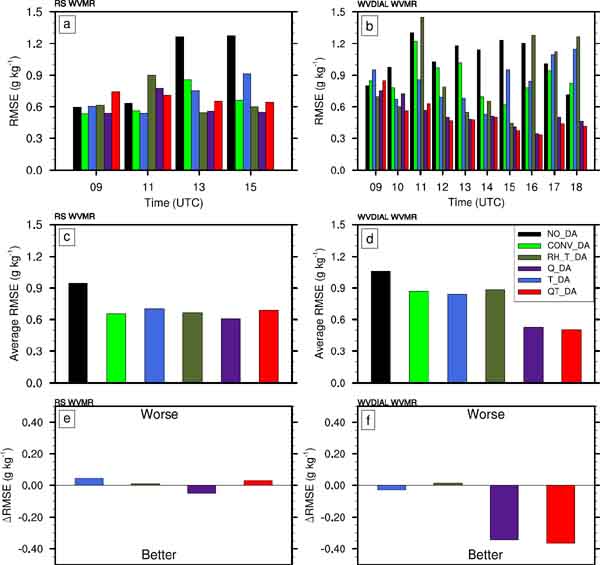
Figures 9a and 9b shows the RMSE with respect to the radiosonde data for all four assimilation times shown in Fig. 8 and the RMSE with respect to lidar data for all ten assimilation times, respectively. The overall average RMSE for each experiment (Figs. 9c, d), and the relative change in the RMSE for other DA experiments with respect to CONV_DA (Figs. 9e, f). At 09 UTC, in Fig. 9c, CONV_DA and T_DA have almost the same RMSE, though the radiosonde temperature profile deviates from the TRL observations slightly in the upper part of the PBL region. At 11 and 13 UTC, the RMSE of T_DA has the lowest value. At 15 UTC, the RMSE is higher due to the difference between the TRL and radiosonde profiles above the PBL which has been discussed earlier. Q_DA, RH_DA, and QT_DA have a slightly higher RMSE than the other two DA runs but show an improvement compared to the NO_DA experiment. Compared to CONV_DA, the relative change in the RMSE (ΔRMSE) in Fig. 9e for T_DA shows a decrease of 0.1 K, but Q_DA, RH_DA, and QT_DA show an increase of 0.5 K, 0.5K, and 0.45 K, respectively.

Fig. 9.

Temperature RMSE of the analyses compared to local radiosonde data not assimilated into the model together with assimilated TRL observations. (a) Comparison of the RMSE at the four assimilation time-steps (09, 11, 13, 15 UTC) with respect to the radiosonde data and (b) comparison of the RMSE with respect to the TRL observations at the 10 assimilation time-steps from 09 UTC to 18 UTC 24 April 2013. (c) and (d) comparison of the overall temperature RMSE for the corresponding time-steps for (a) and (b), respectively. (e) and (f) depict the relative change in the average RMSE of (c) and (d), respectively, compared to the RMSE of CONV_DA.

The RMSE of the analysis compared to the lidar observations is shown in Fig. 9b for all 10 assimilation time-steps. Q_DA, RH_DA, and QT_DA overestimated the temperature during daytime and, hence, the temperature RMSE with respect to the TRL observations increases from the first assimilation to the later cycles and decreases again for the final cycle. Q_DA and RH_DA have a higher RMSE than NO_DA for later cycles. The interesting feature to note here is that when the amount of moisture in the boundary layer is higher—that is, from 0900 UTC to 1100 UTC and from 1400 UTC to 1800 UTC—than between 1200 UTC and 1300 UTC, the assimilation has a higher impact. The RMSE for QT_DA is less than for CONV_DA during this time period. Between 1200 UTC and 1300 UTC, when the moisture in this region is lower, the temperature is overestimated, leading to a higher RMSE during this time. This is again a clear impact of the static nature of the background error covariance. Due to these counteracting impacts of the assimilation at different time-periods, the RMSEs for CONV_DA and QT_DA are similar in magnitude. The T_DA temperature RMSE is mostly constant over the assimilation cycles although there is a decrease of 0.2 K at around 1300 UTC from 0.4 K at 0900 UTC. From Fig. 9f, QT_DA has an increase of less than 0.05 K in ΔRMSE, which means that QT_DA did not worsen CONV_DA much, whereas Q_DA and RH_DA showed an increase of 0.5 K in ΔRMSE. T_DA shows a decrease of 0.7 K in ΔRMSE. In summary, T_DA outperformed all the other experiments in terms of the temperature impact.

4.4 Water vapor mixing ratio

Figure 10 depicts the profiles of the analyzed WVMR at the assimilation time steps 09, 11, 13, and 15 UTC for all the different DA experiments including the observations. The DIAL WVMR observations were limited to a height of 2.5 km since the observation error was higher than the observed value.

Fig. 10.

WVMR profiles of WVDIAL, radiosondes, and analyses at (a) 09 UTC, (b) 11 UTC, (c) 13 UTC, and (d) 15 UTC. The WVDIAL observations (orange) along with their total errors shown by error bars are plotted up to 2500 m AGL. Radiosonde observations (violet) which were not assimilated are plotted for reference. Black: NO_DA, green: CONV_DA, olive green: RH_DA, dark purple: Q_DA, blue: T_DA, and red: QT_DA are shown.

All the assimilation runs do not show much difference from NO_DA in the PBL at 09 UTC. The surface observations were well captured by all the experiments at 11 UTC except for Q_DA which shows insignificant values of WVMR. But in the PBL above the surface layer, Q_DA and QT_DA are in good agreement with the radiosonde and DIAL observations at later time-steps. The Q_DA and QT_DA profiles agree with the radiosonde and DIAL observations at 13 UTC and 15 UTC, whereas NO_DA, CONV_DA, and T_DA have higher values of WVMR in the PBL. The Q_DA and QT_DA profiles are similar to those of the other two assimilation experiments in the surface layer since there were no lidar observations available at those levels. NO_DA shows an overestimation in the WVMR of around 1 g kg⁻¹ in the PBL. RH_DA did not outperform Q_DA and QT_DA as expected although it was close to QT_DA at 09 UTC.

The interfacial layer was best captured by Q_DA and QT_DA at all time-steps apart from the first assimilation time-step at 09 UTC. NO_DA and CONV_DA underestimated the WVMR at all time-steps, whereas T_DA shows a positive deviation at 13 UTC and 15 UTC in the interfacial layer. RH_DA shows a negative deviation at 11 UTC and a positive deviation at 15 UTC. The lower free troposphere impact for Q_DA, RH_DA, and QT_DA is in better agreement with the observations than compared to the other runs, which have mixed results. NO_DA and CONV_DA always have a positive deviation. T_DA has positive and negative deviations at 09 UTC and 15 UTC, respectively, but matches with Q_DA, RH_DA, and QT_DA at 11 UTC and 13 UTC. In short, Q_DA and QT_DA had a more major impact on the WVMR than the other experiments.

Figures 11a and 11b depict the WVMR RMSE compared to the radiosonde observations at 09, 11, 13, and 15 UTC, and the WVMR RMSE compared to the lidar observations at all ten assimilation time steps from 09 UTC to 18 UTC, respectively. The overall average of RMSE for each experiment are shown in Figs. 11c and 11d. The relative change in RMSE for the other DA experiments compared to CONV_DA are shown in Figs. 11e and 11f. Keeping in mind the radiosonde error due to drifting, Q_DA and QT_DA performed better than the other experiments although the difference with T_DA was less. The RMSE for RH_DA is the same as for CONV_DA although slightly better than T_DA and QT_DA. From Fig. 11a, the decline in WVMR RMSE as the assimilation cycle progresses is visible. Although the QT_DA RMSE decline rate is small, the decrease is consistent. Although the overall RMSE for Q_DA and QT_DA is closer to that for T_DA and CONV_DA, it is lower (Fig. 11c). The RMSE differences compared to CONV_DA are considerably less with magnitudes of +0.01 g kg⁻¹ for RH_DA, +0.03 g kg⁻¹ for QT_DA, and +0.05 g kg⁻¹ for T_DA. Q_DA has a difference of −0.05 g kg⁻¹ compared to CONV_DA.

Fig. 11.

WVMR RMSE of the analyses compared to local radiosonde data not assimilated into the model together with assimilated WVDIAL observations. (a) Comparison of the RMSE at the four assimilation time-steps (09, 11, 13, 15 UTC) with respect to the radiosonde data and (b) comparison of the RMSE with respect to the WVDIAL observations at the 10 assimilation time-steps from 09 UTC to 18 UTC 24 April 2013. (c) and (d) compare the overall WVMR RMSE for the corresponding time-steps for (a) and (b), respectively. (e) and (f) depict the relative change in the average RMSE of (c) and (d) respectively, compared to the RMSE of CONV_DA.

Compared to the WVDIAL observations, the RMSEs in the WVMR (Figs. 11b, d) also have a similar declining trend to those seen in the radiosonde comparisons in consecutive assimilation cycles, but the decline is higher. An important difference between the WVDIAL and radiosonde observations which needs to be considered is the error due to the temporal coverage of the two datasets. The WVDIAL dataset gives a complete profile of the atmosphere every 10 s, while the radiosonde provides data only from the point of ascent. The mean rate of ascent of the radiosondes launched during IOP 6 of the HOPE campaign was around 5 m s⁻¹. This means that the time taken for a radiosonde to cross the PBL (taking its height to be 1500 m) would be 5 minutes, which is still 30 times higher than the time required for obtaining a single lidar profile. This temporal resolution is not optimal if the atmosphere is rapidly changing. Hence, the DIAL dataset is a continuous measurement whereas the radiosonde data are instantaneous ones. This also explains the reason why the DIAL dataset does not have such a smooth profile as the radiosonde data because the DIAL data capture all the fluctuations in the atmosphere. Q_DA and QT_DA (Fig. 11b) have the lowest RMSE in all the assimilation cycles; also, the declining trend for the RMSE in the successive assimilations proves that the model successfully corrects the WVMR. T_DA does not show a visible impact for successive assimilations. Hence, the WVMR RMSE for T_DA in Fig. 11b is always higher than for Q_DA and QT_DA. However, the WVMR RMSE for T_DA has a value similar to the CONV_DA. Although RH_DA has lower RMSE values than CONV_DA at 09 UTC and 10 UTC, later cycles have a higher RMSE. In Fig. 11d, the overall RMSE for QT_DA is the lowest for all the experiments. The ΔRMSE in Fig. 11f indicates that there is a decrease of 0.36 g kg⁻¹ for QT_DA and 0.3 g kg⁻¹ for Q_DA but only 0.03 g kg⁻¹ for T_DA when compared to CONV_DA. RH_DA shows an increase of 0.02 g kg⁻¹ compared to CONV_DA. Figure 12 shows an analysis of the difference between QT_DA and CONV_DA. The spatial analysis difference at 09 UTC and 18 UTC on 24 April 2013 are shown in Figs. 12a and 12b, respectively. A vertical cross-section of the analysis difference at 09 UTC is shown in Fig. 12c. In order to analyze the impact of the assimilated lidar data, a 6-hr forecast difference between QT_DA and CONV_DA initiated from 18 UTC is shown in Fig. 12d. However the assimilation impact cannot be due completely to the lidar observations and, presumably, the number of observations in the conventional data should be considered. The spatial analyses shown in Figs. 12a, 12b, and 12d are for a height of 2000 m, which is assumed to be the PBL top, where the impact is significant. The impact of a single lidar profile spreading over an area with a diameter of 300 km shows the potential of a network of lidars. The forecast difference after six hours initiated from 18 UTC (Fig. 12d) clearly shows that the impact of the assimilation is both enduring and stable since the impact of the assimilated lidar data lasts for short-range forecasts and does not lead to significant errors during this forecast range. The six-hour forecast difference does not exceed an absolute value of 1.2 g kg⁻¹ in the areas near the lidar instrument location, which accounts for the stability of the atmosphere after assimilating the thermodynamic lidar data.

Fig. 12.

Analysis of the difference between QT_DA and CONV_DA at (a) 09 UTC and (b) 18 UTC 24 April 2013; (c) shows the vertical cross section of the difference, valid at 09 UTC; (d) is the six-hour forecast difference between QT_DA and CONV_DA initiated from 18 UTC. The spatial distributions are valid at a height of 2000 m ASL.

5. Summary and outlook

In this study, we investigated the impact of assimilating WVMR and temperature data from lidar systems on the vertical structure of temperature and moisture inside the PBL. For this purpose, we applied WRF version 3.8.1 together with its 3DVAR DA system at a convection-permitting horizontal resolution of 2.5 km over central Europe. The DA system was operated in the RUC mode, meaning that the assimilations were hourly. For the present study, lidar data from the HOPE campaign were used for the assimilation. The IOP took place from 0900 UTC to 1800 UTC on the 24 April 2013 in western Germany on a clear-sky day with hardly any optically thick clouds. Temperature data from heights of 500 m to 3000 m above the ground were taken for the experiment. WVMR data were taken from 400 m to 2500 m above the ground level. Data from lower levels had to be discarded due to the overlap error. Apart from the lidar measurements, there were four radiosonde launches at 09, 11, 13 and 15 UTC. The mean of these radiosonde measurements was used for calibrating the TRL and as an independent measurement for comparison with the model output since these radiosonde measurements were not assimilated in the DA system.

Six model runs were conducted for the whole impact study. A run (NO_DA) with no data assimilated, conventional data assimilation (CONV_DA) or the control run with only conventional observations from the ECMWF, TRL data assimilation (T_DA) along with the conventional dataset, WVMR data assimilation (Q_DA) along with the conventional dataset, RH data assimilation (RH_DA) along with the conventional dataset, and finally the WVMR and TRL data assimilation (QT_DA) along with the conventional data.

In this study, we introduced a new forward operator called TDLIDAR for direct WVMR DA, which was developed through the modification of an already-existing operator in the WRFDA system, the AIRSRET operator. Also, separate sensitivity tests were conducted with the QT_DA to study the sensitivity of the newly introduced error factor (max_error_q_DIAL) in the WRFDA registry. SOTs were conducted to analyze the response of the input WVMR and temperature data separately in the DA system. An increase in the WVMR resulted in a subsequent cooling at the point of assimilation in the model. On the other hand, an increase in the temperature resulted in a subsequent drying.

The impact of the assimilation of WVMR and temperature lidar data through the new forward operator was, overall, positive. The input observations were assimilated with a very low number of rejected observations: the model only rejected a few observations during the first assimilation cycle. The WVMR and temperature profiles of the model output indicated that the input lidar observations could correct the first guess during the assimilation process to a reasonable extent. From the results of the five DA runs, we conclude that, the assimilation of both temperature and WVMR lidar observations improved the thermodynamic profiles in the analyses. T_DA and Q_DA improved the temperature and moisture profiles, respectively, whereas QT_DA improved both compared to CONV_DA. RH_DA did not outperform either Q_DA or QT_DA in the study, showing that the TDLIDAR operator leads to a better impact than the RH operator. We quantified the analyses by their RMSE with respect to the assimilated lidar observations as well as independent radiosonde observations. However, the lidar observations were more suitable for model verification than radiosonde data because they point exactly to the zenith rather than along an irregular vertical track. The WVMR RMSE computed with respect to the WVDIAL observations for QT_DA reduced by 40 % compared to those computed for CONV_DA run whereas RH_DA did not show an overall improvement. This highlights that using the forward operator for the data input had a positive impact on the modeled WVMR variable. However, at the same time, the impact on the temperature was reduced due to the significant dependency between the WVMR and temperature variables in the analysis.

In real-time operational forecasting with data assimilated from active remote-sensing instruments like lidars, which provide data with a very low observational bias, a deterministic DA system whose correlation statistics are derived from a set of forecast error differences might not provide the best analysis. With the introduction of a flow-dependent background error-covariance matrix with the help of ensemble-based DA systems, the cross-correlation between the temperature and humidity variables is expected to be a better representative of the real-time scenario. The matrix B in ensemble-based DA systems reflects the dynamic nature of the atmosphere. Thus, we plan to assimilate thermodynamic lidar data with ensemble DA techniques in the future. Furthermore, modules for the conversion of absolute humidity and specific humidity to the WVMR will be incorporated. Currently, with a limited number of lidars, we limited our studies to convective-scale DA. However, in the future, with a larger number of lidars which operate as a network, we can enhance our studies to synoptic-scale DA. We foresee synoptic-scale DA of lidar networks as very beneficial for operational numerical weather forecasting centers.

Acknowledgments

We express our sincere gratitude to the High Performance Computing Centre Stuttgart (HLRS) for providing the necessary computational resources for the completion of the simulations. We are also grateful to the ECMWF for providing the operational analysis data. We also express our sincere gratitude to colleagues from KIT Cube for providing radiosoundings during the IOPs.

Appendix

The total derivative of RH expands as per the equation.

  

After dividing Eq. A1 by RH we get the relative error equation

  

For normal atmospheric conditions

  

We took a normal value of 10 g kg⁻¹ and an error of 1 g kg⁻¹ for the mixing ratio in the numerical example, which are similar to the values for the absolute humidity measurements from the WVDIAL. Similarly, a temperature error of 1.1 K was taken for the TRL measurements. Substituting the above values in Eq. A2, we get these values for the individual terms:

  

The WVMR error δm expands to

  

For normal atmospheric conditions

  

Substituting the above values we get

  

References

•  Adam,  S.,  A.  Behrendt,  T.  Schwitalla,  E.  Hammann, and  V.  Wulfmeyer, 2016: First assimilation of temperature lidar data into an NWP model: Impact on the simulation of the temperature field, inversion strength and PBL depth. Quart. J. Roy. Meteor. Soc., 142, 2882-2896.
•  Apituley,  A.,  K. M.  Wilson,  C.  Potma,  H.  Volten, and  M.  de Graaf, 2009: Performance assessment and application of Caeli — A high-performance Raman lidar for diurnal profiling of water vapour, aerosols and clouds. Proceedings of the 8th International Symposium on Tropospheric Profiling, Delft, Netherlands, S06-O10, 4 pp. [Available at http://projects.knmi.nl/cesar/istp8/data/1753005.pdf.]
•  Aranami,  K.,  T. A.  Hara,  Y. A.  Ikuta,  K. O.  Kawano,  K. E.  Matsubayashi,  H. I.  Kusabiraki,  T. A.  Ito,  T. A.  Egawa,  K. O.  Yamashita,  Y. U.  Ota, and  Y. O.  Ishikawa, 2015: A new operational regional model for convection-permitting numerical weather prediction at JMA. Research activities in atmospheric and oceanic modelling. WCRP Report No. 12/2015,  Astakhova,  E. (ed.), CAS/JSC Working Group on Numerical Experimentation, 2 pp. [Available at 2https://www.wcrpclimate.org/WGNE/BlueBook/2015/individual-articles/05_Aranami_Kohei_asuca.pdf.]
•  Arshinov,  Y.,  S.  Bobrovnikov,  I.  Serikov,  A.  Ansmann,  U.  Wandinger,  D.  Althausen,  I.  Mattis, and  D.  Müller, 2005: Daytime operation of a pure rotational Raman lidar by use of a Fabry–Perot interferometer. Appl. Opt., 44, 3593-3603.
•  Barker,  D. M.,  W.  Huang,  Y.-R.  Guo,  A. J.  Bourgeois, and  Q. N.  Xiao, 2004: A Three-Dimensional Variational Data Assimilation system for MM5: Implementation and initial results. Mon. Wea. Rev., 132, 897-914.
•  Bauer,  H.-S.,  T.  Schwitalla,  V.  Wulfmeyer,  A.  Bakhshaii,  U.  Ehret,  M.  Neuper, and  O.  Caumont, 2015: Quantitative precipitation estimation based on high-resolution numerical weather prediction and data assimilation with WRF – A performance test. Tellus, 67, 25047, doi:10.3402/tellusa.v67.25047.
•  Behrendt,  A., and  J.  Reichardt, 2000: Atmospheric temperature profiling in the presence of clouds with a pure rotational Raman lidar by use of an interference-filter-based polychromator. Appl. Opt., 39, 1372-1378.
•  Behrendt,  A.,  T.  Nakamura, and  T.  Tsuda, 2004: Combined temperature lidar for measurements in the troposphere, stratosphere, and mesosphere. Appl. Opt., 43, 2930, doi:10.1364/ao.43.002930.
•  Behrendt,  A.,  V.  Wulfmeyer,  A.  Riede,  G.  Wagner,  S.  Pal,  H.  Bauer,  M.  Radlach, and  F.  Späth, 2009: Three-dimensional observations of atmospheric humidity with a scanning differential absorption lidar. Remote Sens. Clouds Atmos. XIV, 7475, 74750L, doi:10.1117/12.835143.
•  Behrendt,  A.,  V.  Wulfmeyer,  E.  Hammann,  S. K.  Muppa, and  S.  Pal, 2015: Profiles of second- to fourth-order moments of turbulent temperature fluctuations in the convective boundary layer: First measurements with rotational Raman lidar. Atmos. Chem. Phys., 15, 5485-5500.
•  Benjamin,  S. G.,  S. S.  Weygandt,  J. M.  Brown,  T. L.  Smith,  T.  Smirnova,  W. R.  Moninger,  B.  Schwartz,  E. J.  Szoke, and  K.  Brundage, 2004: An hourly assimilation-forecast cycle: The RUC. Mon. Wea. Rev., 132, 495-518.
•  Benjamin,  S. G.,  S. S.  Weygandt,  J. M.  Brown,  M.  Hu,  C. R.  Alexander,  T. G.  Smirnova,  J. B.  Olson,  E. P.  James,  D. C.  Dowell,  G. A.  Grell, and  H.  Lin, 2016: A North American hourly assimilation and model forecast cycle: The rapid refresh. Mon. Wea. Rev., 144, 1669-1694.
•  Berre,  L., 2000: Estimation of synoptic and mesoscale forecast error covariances in a limited-area model. Mon. Wea. Rev., 128, 644-667.
•  Berre,  L.,  S. E.  Ştefǎnescu, and  M. B.  Pereira, 2006: The representation of the analysis effect in three error simulation techniques. Tellus, 58, 196-209.
•  Bhawar,  R.,  P.  Di Girolamo,  D.  Summa,  C.  Flamant,  D.  Althausen,  A.  Behrendt,  C.  Kiemle,  P.  Bosser,  M.  Cacciani,  C.  Champollion,  T.  Di Iorio,  R.  Engelmann,  C.  Herold,  D.  Müller,  S.  Pal,  M.  Wirth, and  V.  Wulfmeyer, 2011: The water vapour intercomparison effort in the framework of the convective and orographically-induced precipitation study: Airborne-to-ground-based and airborne-to-airborne lidar systems. Quart. J. Roy. Meteor. Soc., 137, 325-348.
•  Bielli,  S.,  M.  Grzeschik,  E.  Richard,  C.  Flamant,  C.  Champollion,  C.  Kiemle,  M.  Dorninger, and  P.  Brousseau, 2012: Assimilation of water-vapour airborne lidar observations: Impact study on the COPS precipitation forecasts. Quart. J. Roy. Meteor. Soc., 138, 1652-1667.
•  Blumberg,  W. G.,  D. D.  Turner,  U.  Löhnert, and  S.  Castleberry, 2015: Ground-based temperature and humidity profiling using spectral infrared and microwave observations. Part II: Actual retrieval performance in clear-sky and cloudy conditions. J. Appl. Meteor. Climatol., 54, 2305-2319.
•  Bolton,  D., 1980: The computation of equivalent potential temperature. Mon. Wea. Rev., 108, 1046-1053.
•  Bösenberg,  J., 1998: Ground-based differential absorption lidar for water-vapor and temperature profiling: Methodology. Appl. Opt., 37, 3845-3860.
•  Brocard,  E.,  R.  Philipona,  A.  Haefele,  G.  Romanens,  A.  Mueller,  D.  Ruffieux,  V.  Simeonov, and  B.  Calpini, 2013: Raman lidar for meteorological observations, RALMO. Part 2: Validation of water vapor measurements. Atmos. Meas. Tech., 6, 1347-1358.
•  Brousseau,  P.,  L.  Berre,  F.  Bouttier, and  G.  Desroziers, 2011: Background-error covariances for a convective-scale data-assimilation system: AROME-France 3D-Var. Quart. J. Roy. Meteor. Soc., 137, 409-422.
•  Browning,  K. A.,  A. M.  Blyth,  P. A.  Clark,  U.  Corsmeier,  C. J.  Morcrette,  J. L.  Agnew,  S. P.  Ballard,  D.  Bamber,  C.  Barthlott,  L. J.  Bennett, and  K. M.  Beswick, 2007: The convective storm initiation project. Bull. Amer. Meteor. Soc., 88, 1939-1955.
•  Cadeddu,  M. P.,  G. E.  Peckham, and  C.  Gaffard, 2002: The vertical resolution of ground-based microwave radiometers analyzed through a multiresolution wavelet technique. IEEE Trans. Geosci. Remote Sens., 40, 531-540.
•  Cooney,  J., 1972: Measurement of atmospheric temperature profiles by Raman backscatter. J. Appl. Meteor., 11, 108-112.
•  Courtier,  P.,  E.  Andersson,  W.  Heckley,  D.  Vasiljevic,  M.  Hamrud,  A.  Hollingsworth,  F.  Rabier,  M.  Fisher, and  J.  Pailleux, 1998: The ECMWF implementation of three-dimensional variational assimilation (3D-Var). I: Formulation. Quart. J. Roy. Meteor. Soc., 124, 1783-1807.
•  Crook,  N. A., 1996: Sensitivity of moist convection forced by boundary layer processes to low-level thermodynamic fields. Mon. Wea. Rev., 124, 1767-1785.
•  Dailey,  P. S., and  R. G.  Fovell, 1999: Numerical simulation of the interaction between the sea-breeze front and horizontal convective rolls. Part I: Offshore ambient flow. Mon. Wea. Rev., 127, 858-878.
•  Di Girolamo,  P.,  R.  Marchese,  D. N.  Whiteman, and  B. B.  Demoz, 2004: Rotational Raman Lidar measurements of atmospheric temperature in the UV. Geophys. Res. Lett., 31, L01106, doi:10.1029/2003GL018342.
•  Dinoev,  T.,  V.  B. Simeonov,  Y.  Arshinov,  S.  Bobrovnikov,  P.  Ristori,  B.  Calpini,  M.  Parlange, and  H.  van den Bergh, 2013: Raman Lidar for meteorological observations, RALMO. Part 1: Instrument description. Atmos. Meas. Tech., 6, 1329-1346.
•  Dixon,  M.,  Z.  Li,  H.  Lean,  N.  Roberts, and  S.  Balland, 2009: Impact of data assimilation on forecasting convection over the United Kingdom using a high-resolution version of the met office unified model. Mon. Wea. Rev., 137, 1562-1584.
•  Donlon,  C. J.,  M.  Martin,  J.  Stark,  J.  Roberts-Jones,  E.  Fiedler, and  W.  Wimmer, 2012: The Operational Sea Surface Temperature and Sea Ice Analysis (OSTIA) system. Remote Sens. Environ., 116, 140-158.
•  Engelbart,  D. A. M., and  E.  Haas, 2006: LAUNCH-2005-International Lindenberg campaign for assessment of humidity and cloud profiling systems and its impact on high-resolution modelling. Proceeding of 7th International Symposium on Tropospheric profiling: Needs and technologies, 11-17.
•  Evensen,  G., 2003: The ensemble Kalman filter: Theoretical formulation and practical implementation. Ocean Dyn., 53, 343-367.
•  Fischer,  L., 2013: Statistical characterisation of water vapour variability in the troposphere. Doctoral dissertation, Ludwig Maximilian University of Munich, Germany, 124 pp. [Available at https://edoc.ub.unimuenchen.de/16208/1/Fischer_Lucas.pdf.]
•  Fisher,  M., 2003: Background error covariance modelling. Seminar on Recent Development in Data Assimilation for Atmosphere and Ocean, 45-63.
•  Geerts,  B.,  D.  Parsons,  C. L.  Ziegler,  T. M.  Weckwerth,  M. I.  Biggerstaff,  R. D.  Clark,  M. C.  Coniglio,  B. B.  Demoz,  R. A.  Ferrare,  W. A.  Gallus, Jr.,  K.  Haghi,  J. M.  Hanesiak,  P. M.  Klein,  K. R.  Knupp,  K.  Kosiba,  G. M.  McFarquhar,  J. A.  Moore,  A. R.  Nehrir,  M. D.  Parker,  J. O.  Pinto,  R. M.  Rauber,  R. S.  Schumacher,  D. D.  Turner,  Q.  Wang,  X.  Wang,  Z.  Wang, and  J.  Wurman, 2017: The 2015 plains elevated convection at night field project. Bull. Amer. Meteor. Soc., 98, 767-786.
•  Goldsmith,  J. E. M.,  F. H.  Blair,  S. E.  Bisson, and  D. D.  Turner, 1998: Turn-key Raman lidar for profiling atmospheric water vapor, clouds, and aerosols. Appl. Opt., 37, 4979-4990.
•  Grzeschik,  M.,  H. S.  Bauer,  V.  Wulfmeyer,  D.  Engelbart,  U.  Wandinger,  I.  Mattis,  D.  Althausen,  R.  Engelmann,  M.  Tesche, and  A.  Riede, 2008: Four-dimensional variational data analysis of water vapor Raman lidar data and their impact on mesoscale forecasts. J. Atmos. Oceanic Technol., 25, 1437-1453.
•  Gustafsson,  N.,  T.  Janjić,  C.  Schraff,  D.  Leuenberger,  M.  Weissmann,  H.  Reich,  P.  Brousseau,  T.  Montmerle,  E.  Wattrelot,  A.  Bučánek, and  M.  Mile, 2018: Survey of data assimilation methods for convective-scale numerical weather prediction at operational centres. Quart. J. Roy. Meteor. Soc., 144, 1218-1256.
•  Hammann,  E.,  A.  Behrendt,  F.  Le Mounier, and  V.  Wulfmeyer, 2015: Temperature profiling of the atmospheric boundary layer with rotational Raman lidar during the HD(CP)² Observational Prototype Experiment. Atmos. Chem. Phys., 15, 2867-2881.
•  Harnisch,  F.,  M.  Weissmann,  C.  Cardinali, and  M.  Wirth, 2011: Experimental assimilation of DIAL water vapour observations in the ECMWF global model. Quart. J. Roy. Meteor. Soc., 137, 1532-1546.
•  Hollingsworth,  A., and  P.  Lönnberg, 1986: The statistical structure of short-range forecast errors as determined from radiosonde data. Part I: The wind field. Tellus A, 38, 111-136.
•  Honda,  Y.,  M.  Nishijima,  K.  Koizumi,  Y.  Ohta,  K.  Tamiya,  T.  Kawabata, and  T.  Tsuyuki, 2006: A pre-operational variational data assimilation system for a non-hydrostatic model at the Japan Meteorological Agency: Formulation and preliminary results. Quart. J. Roy. Meteor. Soc., 131, 3465-3475.
•  Hong,  S.-Y.,  H.  Park,  H. B.  Cheong,  J. E. E.  Kim,  M. S.  Koo,  J.  Jang,  S.  Ham,  S. O.  Hwang,  B. K.  Park,  E. C.  Chang, and  H.  Li, 2013: The global/regional integrated model system (GRIMs). Asia-Pacific J. Atmos. Sci., 49, 219-243.
•  Horváth,  Á.,  O.  Hautecoeur,  R.  Borde,  H.  Deneke, and  S. A.  Buehler, 2017: Evaluation of the EUMETSAT global AVHRR wind product. J. Appl. Meteor. Climatol., 56, 2353-2376.
•  Hu,  M.,  M.  Xue, and  K.  Brewster, 2006: 3DVAR and cloud analysis with WSR-88D level-II data for the prediction of the Fort Worth, Texas, tornadic thunderstorms. Part I: Cloud analysis and its impact. Mon. Wea. Rev., 134, 675-698.
•  Hu,  M.,  S. G.  Benjamin,  T. T.  Ladwig,  D. C.  Dowell,  S. S.  Weygandt,  C. R.  Alexander, and  J. S.  Whitaker, 2017: GSI three-dimensional ensemble-variational hybrid data assimilation using a global ensemble for the regional rapid refresh model. Mon. Wea. Rev., 145, 4205-4225.
•  Huang,  X. Y.,  Q.  Xiao,  D. M.  Barker,  X.  Zhang,  J.  Michalakes,  W.  Huang,  T.  Henderson,  J.  Bray,  Y.  Chen,  Z. M. J.  Dudhia,  Y.  Guo,  X.  Zhang,  D.-J.  Won,  H.-C.  Lin, and  Y.-H.  Kuo, 2009: Four-dimensional variational data assimilation for WRF: Formulation and preliminary results. Mon. Wea. Rev., 137, 299-314.
•  Iacono,  M. J.,  J. S.  Delamere,  E. J.  Mlawer,  M. W.  Shephard,  S. A.  Clough, and  W. D.  Collins, 2008: Radiative forcing by long-lived greenhouse gases: Calculations with the AER radiative transfer models. J. Geophys. Res., 113, D13103, doi:10.1029/2008JD009944.
•  Ingleby,  B., 2017: An assessment of different radiosonde types 2015/2016. ECMWF Tech. Memo., No. 87, 71 pp, doi:10.21957/0nje0wpsa.
•  Ingleby,  N. B.,  A. C.  Lorenc,  K.  Ngan,  F.  Rawlins, and  D. R.  Jackson, 2013: Improved variational analyses using a nonlinear humidity control variable. Quart. J. Roy. Meteor. Soc., 139, 1875-1887.
•  Ismail,  S., and  E. V  Browell, 1989: Airborne and spaceborne lidar measurements of water vapor profiles: a sensitivity analysis; erratum. Appl. Opt., 28, 4981, doi: 10.1364/ao.28.004981.
•  Janjic,  Z. I., 2003: A nonhydrostatic model based on a new approach. Meteor. Atmos. Phys., 82, 271-285.
•  Kalthoff,  N.,  B.  Adler,  A.  Wieser,  M.  Kohler,  K.  Träumner,  J.  Handwerker,  U.  Corsmeier,  S.  Khodayar,  D.  Lambert,  A.  Kopmann,  N.  Kunka,  G.  Dick,  M.  Ramatschi,  J.  Wickert, and  C.  Kottmeier, 2013: KITcube - A mobile observation platform for convection studies deployed during HyMeX. Meteor. Z., 22, 633-647.
•  Kingsmill,  D. E., 1995: Convection initiation associated with a sea-breeze front, a gust front, and their collision. Mon. Wea. Rev., 123, 2913-2933.
•  Lange,  D.,  A.  Behrendt, and  V.  Wulfmeyer, 2018: Compact automatic rotational Raman lidar system for continuous day- and nighttime temperature and humidity mapping. Proceeding of 20th EGU General Assembly, EGU2018, 4–13 April, 2018, Vienna, Austria, 9114-9114.
•  Lee,  B. D.,  R. D.  Farley, and  M. R.  Hjelmfelt, 1991: A numerical case study of convection initiation along colliding convergence boundaries in northeast Colorado. J. Atmos. Sci., 48, 2350-2366.
•  Lenschow,  D. H.,  V.  Wulfmeyer, and  C.  Senff, 2000: Measuring second- through fourth-order moments in noisy data. J. Atmos. Oceanic Technol., 17, 1330-1347.
•  Lorenc,  A. C., 2003: The potential of the ensemble Kalman filter for NWP – A comparison with 4D-Var. Quart. J. Roy. Meteor. Soc., 129, 3183-3203.
•  Macke,  A.,  Seifert,  P.  Baars,  H.  Barthlott,  C.  Beekmans,  C.  Behrendt,  A.  Behrendt,  B.  Bohn,  M.  Brueck,  J.  Bühl,  S.  Crewell,  T.  Damian,  H.  Deneke,  S.  Düsing,  A.  Foth,  P.  DiGirolamo,  E.  Hammann,  R.  Heinze,  A.  Hirsikko,  J.  Kalisch,  N.  Kalthoff,  S.  Kinne,  M.  Kohler,  U.  Löhnert,  B. L.  Madhavan,  V.  Maurer,  S. K.  Muppa,  J.  Schween,  I.  Serikov,  H.  Siebert,  C.  Simmer,  F.  Späth,  S.  Steinke,  K.  Träumner,  S.  Trömel,  B.  Wehner,  A.  Wieser,  V.  Wulfmeyer, and  X.  Xie, 2017: The HD (CP)² observational prototype experiment (HOPE)–An overview. Atmos. Chem. Phys., 17, 4887-4914.
•  Metzendorf,  S., 2019: 10 W-Average-Power Single-Frequency Ti:sapphire laser with tuning agility–A breakthrough in high-resolution 3D water-vapor measurement. Doctoral dissertation, University of Hohenheim of Stuttgart, Germany, 242 pp. [Available at http://opus.uni-hohenheim.de/volltexte/2019/1558/pdf/Metzendorf_2018_Dissertation_Hohenheim.pdf.]
•  Muppa,  S. K.,  A.  Behrendt,  F.  Späth,  V.  Wulfmeyer,  S.  Metzendorf, and  A.  Riede, 2016: Turbulent humidity fluctuations in the convective boundary layer: Case studies using water vapour differential absorption lidar measurements. Bound.-Layer Meteor., 158, 43-66.
•  Muppa,  S. K.,  A.  Behrendt,  H.-S.  Bauer,  F.  Späth,  R.  Heinze,  C.  Moseley, and  V.  Wulfmeyer, 2018: Characterizing the turbulent higher-order moments in the convective boundary layer: Evaluation of large eddy simulations with high-resolution lidar observations. Proceeding of 20th EGU General Assembly, EGU2018, 4–13 April, 2018, Vienna, Austria, 14632-14632.
•  Murphey,  H. V.,  R. M.  Wakimoto,  C.  Flamant, and  D. E.  Kingsmill, 2006: Dryline on 19 June 2002 during IHOP. Part I: Airborne Doppler and LEANDRE II analyses of the thin line structure and convection initiation. Mon. Wea. Rev., 134, 406-430.
•  Nakanishi,  M., and  H.  Niino, 2006: An improved Mellor-Yamada Level-3 model: Its numerical stability and application to a regional prediction of advection fog. Bound.-Layer Meteor., 119, 397-407.
•  Nakanishi,  M., and  H.  Niino, 2009: Development of an improved turbulence closure model for the atmospheric boundary layer. J. Meteor. Soc. Japan, 87, 895-912.
•  Niu,  G. Y.,  Z. L.  Yang,  K. E.  Mitchell,  F.  Chen,  M. B.  Ek,  M.  Barlage,  A.  Kumar,  K.  Manning,  D.  Niyogi,  E.  Rosero,  M.  Tewari, and  Y.  Xia, 2011: The community Noah land surface model with multiparameterization options (Noah-MP): 1. Model description and evaluation with local-scale measurements. J. Geophys. Res.: Atmos., 116, D12109, doi:10.1029/2010JD015139.
•  Parrish,  D. F., and  J. C.  Derber, 1992: The National Meteorological Center's spectral statistical-interpolation analysis system. Mon. Wea. Rev., 120, 1747-1763.
•  Powers,  J. G.,  J. B.  Klemp,  W. C.  Skamarock,  C. A.  Davis,  J.  Dudhia,  D. O.  Gill,  J. L.  Coen,  D. J.  Gochis,  R.  Ahmadov,  S. E.  Peckham,  G. A.  Grell,  J.  Michalakes,  S.  Trahan,  S. G.  Benjamin,  C. R.  Alexander,  G. J.  Dimego,  W.  Wang,  C. S.  Schwartz,  G. S.  Romine,  Z.  Liu,  C.  Snyder,  F.  Chen,  M. J.  Barlage,  W.  Yu, and  M. G.  Duda, 2017: The weather research and forecasting model: Overview, system efforts, and future directions. Bull. Amer. Meteor. Soc., 98, 1717-1737.
•  Radlach,  M.,  A.  Behrendt, and  V.  Wulfmeyer, 2008: Scanning rotational Raman lidar at 355 nm for the measurement of tropospheric temperature fields. Atmos. Chem. Phys., 8, 159-169.
•  Reichardt,  J.,  U.  Wandinger,  V.  Klein,  I.  Mattis,  B.  Hilber, and  R.  Begbie, 2012: RAMSES: German Meteorological Service autonomous Raman lidar for water vapor, temperature, aerosol, and cloud measurements. Appl. Opt., 51, 8111-8131.
•  Richard,  E.,  A.  Buzzi, and  G.  Zängl, 2007: Quantitative precipitation forecasting in the Alps: The advances achieved by the Mesoscale Alpine Programme. Quart. J. Roy. Meteor. Soc., 133, 831-846.
•  Santanello,  J. A.,  P. A.  Dirmeyer,  C. R.  Ferguson,  K. L.  Findell,  A. B.  Tawfik,  A.  Berg,  M.  Ek,  P.  Gentine,  B. P.  Guillod,  C.  van Heerwaarden,  J.  Roundy, and  V.  Wulfmeyer, 2018: Land-atmosphere interactions: The LoCo perspective. Bull. Amer. Meteor. Soc., 99, 1253-1272.
•  Savitzky,  A., and  M. J. E.  Golay, 1964: Smoothing and differentiation of data by simplified least squares procedures. Anal. Chem., 36, 1627-1639.
•  Schotland,  R. M., 1966: Some observations of the vertical profile of water vapor by means of a laser optical radar (measurement and theory, including signal to noise and transfer function calculations, of atmospheric water vapor using ruby laser optical radar). Proceeding of the 4th Symposium on Remote Sensing of Environment, Rev. Edition, 4864-11-X, Ann Arbor, MI, Willow Run Lab., Inst. Sci. & Technol., Univ. of Michigan, 273-283.
•  Schraff,  C.,  H.  Reich,  A.  Rhodin,  A.  Schomburg,  K.  Stephan,  A.  Periáñez, and  R.  Potthast, 2016: Kilometre-scale ensemble data assimilation for the COSMO model (KENDA). Quart. J. Roy. Meteor. Soc., 142, 1453-1472.
•  Schwitalla,  T., and  V.  Wulfmeyer, 2014: Radar data assimilation experiments using the IPM WRF Rapid Update Cycle. Meteor. Z., 23, 79-102.
•  Schwitalla,  T.,  H. S.  Bauer,  V.  Wulfmeyer, and  F.  Aoshima, 2011: High-resolution simulation over Central Europe: Assimilation experiments during COPS IOP 9c. Quart. J. Roy. Meteor. Soc., 137, 156-175.
•  Schwitalla,  T.,  H. S.  Bauer,  V.  Wulfmeyer, and  K.  Warrach-Sagi, 2017: Continuous high-resolution midlatitude-belt simulations for July–August 2013 with WRF. Geosci. Model Dev., 10, 2031-2055.
•  Skamarock,  W. C.,  J. B.  Klemp,  J.  Dudhia,  D. O.  Gill,  D. M.  Barker,  W.  Wang, and  J. G.  Powers, 2008: A description of the advanced research WRF Version 3. NCAR Technical Note, NCAR/TN-475+STR. University Corporation for Atmospheric Research, 113 pp, doi: 10.5065/D68S4MVH.
•  Späth,  F.,  A.  Behrendt,  S. K.  Muppa,  S.  Metzendorf,  A.  Riede, and  V.  Wulfmeyer, 2014: High-resolution atmospheric water vapor measurements with a scanning differential absorption lidar. Atmos. Chem. Phys. Discuss., 14, 29057-29099.
•  Späth,  F.,  A.  Behrendt,  S.  Kumar Muppa,  S.  Metzendorf,  A.  Riede, and  V.  Wulfmeyer, 2016: 3-D water vapor field in the atmospheric boundary layer observed with scanning differential absorption lidar. Atmos. Meas. Tech., 9, 1701-1720.
•  Späth,  F.,  S.  Metzendorf,  S. K.  Muppa,  A.  Behrendt, and  V.  Wulfmeyer, 2018: Investigation of Humidity Structures from the Land-Surface to the Lower Troposphere Using a Scanning DIAL. Proceedings of 20th EGU General Assembly, EGU2018, 4–13 April, 2018, Vienna, Austria, 15198-15198.
•  Spuler,  S. M.,  K. S.  Repasky,  B.  Morley,  D.  Moen,  M.  Hayman, and  A. R.  Nehrir, 2015: Field-deployable diode-laser-based differential absorption lidar (DIAL) for profiling water vapor. Atmos. Meas. Tech., 8, 1073-1087.
•  Stevens,  B., and  S.  Bony, 2013: What are climate models missing? Science, 340, 1053-1054.
•  Talbot,  C.,  E.  Bou-Zeid, and  J.  Smith, 2012: Nested mesoscale large-eddy simulations with WRF: Performance in real test cases. J. Hydrometeor., 13, 1421-1441.
•  Thompson,  G.,  P. R.  Field,  R. M.  Rasmussen, and  W. D.  Hall, 2008: Explicit forecasts of winter precipitation using an improved bulk microphysics scheme. Part II: Implementation of a new snow parameterization. Mon. Wea. Rev., 136, 5095-5115.
•  Turner,  D. D., and  J. E. M.  Goldsmith, 1999: 24-Hour Raman lidar measurements during the Atmospheric Radiation Measurement program's 1996 and 1997 water vapor intensive observation periods. J. Atmos. Oceanic Technol., 16, 1062-1076.
•  Turner,  D. D., and  U.  LöHnert, 2014: Information content and uncertainties in thermodynamic profiles and liquid cloud properties retrieved from the ground-based Atmospheric Emitted Radiance Interferometer (AERI). J. Appl. Meteor. Climatol., 53, 752-771.
•  Wagner,  G.,  V.  Wulfmeyer, and  A.  Behrendt, 2011: Detailed performance modeling of a pulsed high-power single-frequency Ti:sapphire laser. Appl. Opt., 50, 5921-5937.
•  Wagner,  G.,  A.  Behrendt,  V.  Wulfmeyer,  F.  Späth, and  M.  Schiller, 2013: High-power Ti:sapphire laser at 820 nm for scanning ground-based water–vapor differential absorption lidar. Appl. Opt., 52, 2454-2469.
•  Weckwerth,  T. M., and  D. B.  Parsons, 2006: A review of convection initiation and motivation for IHOP_2002. Mon. Wea. Rev., 134, 5-22.
•  Weckwerth,  T. M.,  J. W.  Wilson, and  R. M.  Wakimoto, 1996: Thermodynamic variability within the convective boundary layer due to horizontal convective rolls. Mon. Wea. Rev., 124, 769-784.
•  Weckwerth,  T. M.,  V.  Wulfmeyer,  R. M.  Wakimoto,  R. M.  Hardesty,  J. W.  Wilson, and  R. M.  Banta, 1999: NCAR–NOAA lower-tropospheric water vapor workshop. Bull. Amer. Meteor. Soc., 80, 2339-2357.
•  Weckwerth,  T. M.,  K. J.  Weber,  D. D.  Turner, and  S. M.  Spuler, 2016: Validation of a water vapor micropulse differential absorption lidar (DIAL). J. Atmos. Oceanic Technol., 33, 2353-2372.
•  Wei,  J.,  O.  Branch,  H.-S.  Bauer,  H.-D.  Wizemann, and  V.  Wulfmeyer, 2017: Impact of enhanced hydrological processes on land-atmosphere feedbacks for the Attert catchment in Luxembourg – LES runs with WRF-Hydro-NOAH-MP vs. WRF-NOAH-MP. Proceedings of 20th EGU General Assembly, EGU2018, 4–13 April, 2018, Vienna, Austria, 16392-16392.
•  Weisman,  M. L.,  C.  Davis,  W.  Wang,  K. W.  Manning, and  J. B.  Klemp, 2008: Experiences with 0-36-h explicit convective forecasts with the WRF-ARW model. Wea. Forecasting, 23, 407-437.
•  Wu,  W. S.,  D. F.  Parrish,  E.  Rogers, and  Y.  Lin, 2017: Regional ensemble-variational data assimilation using global ensemble forecasts. Wea. Forecasting, 32, 83-96.
•  Wulfmeyer,  V., and  J.  Bösenberg, 1998: Ground-based differential absorption lidar for water-vapor profiling: Assessment of accuracy, resolution, and meteorological applications. Appl. Opt., 37, 3825-3844.
•  Wulfmeyer,  V.,  H. S.  Bauer,  M.  Grzeschik,  A.  Behrendt,  F.  Vandenberghe,  E. V  Browell,  S.  Ismail, and  R. A.  Ferrare, 2006: Four-dimensional variational assimilation of water vapor differential absorption lidar data: The first case study within IHOP_2002. Mon. Wea. Rev., 134, 209-230.
•  Wulfmeyer,  V.,  A.  Behrendt,  C.  Kottmeier,  U.  Corsmeier,  C.  Barthlott,  G. C.  Craig,  M.  Hagen,  D.  Althausen,  F.  Aoshima,  M.  Arpagaus,  H. S.  Bauer,  L.  Bennett,  A.  Blyth,  C.  Brandau,  C.  Champollion,  S.  Crewell,  G.  Dick,  P. D.  Girolamo,  M.  Dorninger,  Y.  Dufournet,  R.  Eigenmann,  R.  Engelmann,  C.  Flamant,  T.  Foken,  T.  Gorgas,  M.  Grzeschik,  J.  Handwerker,  C.  Hauck,  H.  Höller,  W.  Junkermann,  N.  Kalthoff,  C.  Kiemle,  S.  Klink,  M.  König,  L.  Krauss,  C. N.  Long,  F.  Madonna,  S.  Mobbs,  B.  Neininger,  S.  Pal,  G.  Peters,  G.  Pigeon,  E.  Richard,  M. W.  Rotach,  H.  Russchenberg,  T.  Schwitalla,  V.  Smith,  R.  Steinacker,  J.  Trentmann,  D. D.  Turner,  J. V.  Baelen,  S.  Vogt,  H.  Volkert,  T.  Weckwerth,  H.  Wernli,  A.  Wieser, and  M.  Wirth, 2011: The Convective and Orographically-induced Precipitation Study (COPS): The scientific strategy, the field phase, and research highlights. Quart. J. Roy. Meteor. Soc., 137, 3-30.
•  Wulfmeyer,  V.,  R. M.  Hardesty,  D. D.  Turner,  A.  Behrendt,  M. P.  Cadeddu,  P.  Di Girolamo,  P.  Schlüssel,  J.  Van Baelen, and  F.  Zus, 2015: A review of the remote sensing of lower tropospheric thermodynamic profiles and its indispensable role for the understanding and the simulation of water and energy cycles. Rev. Geophys., 53, 819-895.
•  Wulfmeyer,  V.,  S. K.  Muppa,  A.  Behrendt,  E.  Hammann,  F.  Späth,  Z.  Sorbjan,  D. D.  Turner, and  R. M.  Hardesty, 2016: Determination of convective boundary layer entrainment fluxes, dissipation rates, and the molecular destruction of variances: Theoretical description and a strategy for its confirmation with a novel lidar system synergy. J. Atmos. Sci., 73, 667-692.
•  Wulfmeyer,  V.,  D. D.  Turner,  B.  Baker,  R.  Banta,  A.  Behrendt,  T.  Bonin,  W. A.  Brewer,  M.  Buban,  A.  Choukulkar,  E.  Dumas R.,  M.  Hardesty,  T.  Heus,  J.  Ingwersen,  D.  Lange,  T. R.  Lee,  S.  Metzendorf,  S. K.  Muppa,  T.  Meyers,  R.  Newsom,  M.  Osman,  S.  Raasch,  J.  Santanello,  C.  Senff,  F.  Späth,  T.  Wagner, and  T.  Weckwerth, 2018: A new research approach for observing and characterizing land–atmosphere feedback. Bull. Amer. Meteor. Soc., 99, 1639-1667.
•  Yang,  Z. L.,  G.-Y.  Niu,  K. E.  Mitchell,  K. E.  Mitchell,  F.  Chen,  M. B.  Ek,  M.  Barlage,  L.  Longuevergne,  K.  Manning,  D.  Niyogi,  M.  Tewari, and  Y.  Xia, 2011: The community Noah land surface model with multiparameterization options (Noah-MP): 2. Evaluation over global river basins. J. Geophys. Res.: Atmos., 116, D12110, doi:10.1029/2010JD015140.
•  Yoshida,  S.,  S.  Yokota,  H.  Seko,  T.  Sakai, and  T.  Nagai, 2020: Observation system simulation experiments of water vapor profiles observed by Raman lidar using LETKF system. SOLA, 16, 43-50.