Abstract
While the terrain-following (sigma) system of representing topography in atmospheric models has been dominant for about the last 60 years, already half a century ago problems using the system were reported in areas of steep topography. A number of schemes had been proposed to address these problems. However, when topography steepness exceeds a given limit all these schemes except the vertical interpolation of the pressure gradient begin to use model information that for physical reasons they should not use.
A radical departure from the system was that of the step-topography eta; but its attractiveness was reduced by the discovery of the corner separation problem. The shaved-cell scheme, nowadays referred to as cut-cell, was free of that problem, and was tested subsequently in idealized as well as real case experiments with encouraging results. The eta discretization has lately been refined to make it also a cut-cell scheme. Another method referred to usually as immersed boundary method enabling treatment of terrain as complex as urban landscape came from computational fluid dynamics. It was made available coupled to the atmospheric Weather Research and Forecasting model.
Results of recent experiments of the cut-cell Eta driven by European Centre for Medium-Range Weather Forecasts (ECMWF) ensemble members are analyzed. In these experiments, all cut-cell Eta members achieved better verification scores with respect to 250 hPa wind speed than their ECMWF driver members. This occurred when an upper-tropospheric trough was crossing the Rocky Mountains barrier. These results are considerably less favorable for the Eta when switched to use sigma, i.e., Eta/sigma, pointing to the benefits of using topography intersecting as opposed to terrain-following systems. But even so the Eta/sigma shows an advantage over its driver members, suggesting that its other features deserve attention.
1. Introduction
Quite a few years back, the first author recalls Eugenia Kalnay (personal communication) referring to the representation of topography as “the perennial vertical coordinate problem”. In spite of a flurry of new methods during the last decade or two, that assessment seems to be more true now than ever. The terrain-following system of Phillips (1957), or as modified to use elevation by Gal-Chen and Somerville (1975), in one of its hybrid flavors, dominates in spite of being introduced more than half a century ago, and with widespread awareness of its limits as the steepness of topography is increasing with increasing horizontal resolution (e.g., Allen 2007, among others). But promising new methods clearly deserve attention. One of them, the “immersed boundary method”, because of its ability to treat vertical terrain boundaries, unacceptable for terrain-following systems. This obviously is very useful for many applications (e.g., Smolarkiewicz et al. 2007). Also the terrain-intersecting cut-cell method, introduced by Adcroft et al. (1997), has perhaps convincingly demonstrated its advantage over the terrain-following approach.
We shall limit ourselves to the representation of topography as it is generally considered a subject of the dynamical cores of atmospheric and ocean models. We will not cover the impacts of the properties of the subgrid scale topography on the surface layer, form drag, and gravity wave drag parameterizations as they tend to be referred to as model “physics” (e.g., Teixeira 2014, among others).
We shall first, in Section 2, summarize the history of the terrain-following method, focusing on ideas that had an impact and/or are used in present day models. In Section 3 we shall summarize the main points of the immersed boundary method (IBM) that accepts the terrain boundary as given to the model, and handles the problem by developing boundary condition schemes to deal with it. Next, we shall review the shaved cell, nowadays referred to as the cut-cell method, along with various tests and results obtained. In Section 4 we shall expand on results achieved by driving the cut-cell Eta model by ECMWF ensemble members, reported earlier in Mesinger and Veljovic (2017). Section 5 will contain our summarizing discussion and comments.
2. Terrain-following systems
While the results of the first successful integration of the atmospheric dynamical equations were published in 1950, followed by the first operational implementation in 1954, it still took some time for the skill of these integrations to become competitive and then superior to that of classical synoptic methods. This occurred perhaps only in the late sixties, along with the development of first general circulation models, GCMs. By that time the suggestion of Phillips (1957) for using a terrain-following (“sigma”) system for the representation of topography had become generally accepted. Rudimentary early efforts in using alternative systems such as pressure or height (e.g., Phillips 1957) received no attention for quite some time. However the first comprehensive GCM effort led to the realization that the sigma system is also not problem free because it involves difficulties with calculation of the pressure-gradient force in places of steep terrain (Kurihara 1968, crediting a suggestion by Smagorinsky et al. 1967). Kurihara's method of vertical interpolation of the geopotential was later rediscovered by Mahrer (1984). A number of other methods have been proposed as well (summarized, e.g., in Mesinger and Janjić 1985; see also Mesinger et al. 2012). A comprehensive and very recent review section of Chow et al. (2019) should be noted here as well.
One might also mention the existence of two versions of terrain-following systems: Phillips' pressure-based version, now in the era of mostly nonhydrostatic models formulated using “hydrostatically-based pressure”, or “mass-based pressure”; and Gal-Chen and Somerville's (1975) height-based version. They are largely equivalent, with the former going from zero at pressure p = 0 to 1 at the surface, and the latter going from 0 at the model's topographic height, to elevation H at the model top. Yet there can be advantages in the height-based choice, one being that the location of velocity grid points does not change with time, a feature that with some model designs results in increased computational efficiency. Still other advantages may present themselves as the horizontal resolution and accordingly the steepness of model topography are increased; note the issues discussed by Husain et al. (2019), documenting improved ability to accept steep model topography resulting from a reformulation of the dynamical core of the Global Environmental Multiscale (GEM) model to use a height-based as opposed to a pressure-based terrain-following coordinate. In addition, it is generally understood that height based models enable simpler nonhydrostatic formulations than pressure based models.
With some vertical discretizations, such as that of the mid-sixties and later UCLA GCM, the original Phillips' sigma coordinate definition
with p denoting pressure, and subscript S standing for surface values, was not usable because the discretization required definitions of layer interfaces as opposed to levels. Therefore, for the UCLA GCM the definition (1) was modified to
with pT being pressure at the model top. Later, it was changed to a form in which pT in (2) was replaced by an interface pressure, pI, with the pressure coordinate used above (Arakawa and Lamb 1977). Using a sigma-like coordinate up to a chosen pressure level and continuing with pressure above that was in fact suggested earlier by Sangster (1960) aiming to facilitate the traditional use of synoptic pressure charts. More recently Simmons and Burridge (1981) introduced a flexible scheme for a smooth transition to pressure, naming it a hybrid coordinate. Note a summary of its features in Thuburn (2011). The hybrid coordinate is now in widespread use in one or another of its variants, aiming to minimize the unnecessary imprint of small-scale topography features as one moves to the higher troposphere and above.
Kurihara (1968) had already noted that the vertical interpolation did not fully eliminate discretization errors above steep topography, and numerous efforts at finding an improved or better remedy ensued. Corby et al. (1972) designed a pressure gradient force scheme which will have no errors when temperature is changing linearly with ln p. Following in the footsteps of Smagorinsky et al. (1967) and Kurihara (1968), Tomine and Abe (1982) suggested a higher order interpolation scheme and reported on considerable reduction of errors in idealized examples compared to several other methods they refer to. Many more schemes were proposed in these early times and were tested on idealized temperature profiles, e.g., see summaries in Mesinger and Janjić (1985), among others. For still more in also addressing and in fact emphasizing oceanic modeling, see Shchepetkin and McWilliams (2003).
A few words might be appropriate as to what is meant by steep topography. At resolutions of the sixties by today's standards topography would not have been steep at any place. With no special schemes used addressing the problems arising from the steepness of topography, Vionnet et al. (2015) found it necessary to filter their already filtered topography so as to remove slopes higher than 45° to prevent instabilities. Still steeper topographies were demonstrated acceptable by Smolarkiewicz et al. (2007), and Zängl (2012), using approaches and/or techniques specifically addressing the issue. We shall summarize or touch upon those later.
The change from pressure to σ coordinates results in the following expression for the pressure gradient force
with φ being geopotential, R the gas constant, and T temperature. The fact that components of the two terms on the right side above, in the direction of steep topography, compared to the left side can have very large magnitudes but opposite signs, led numerous authors (e.g., Kasahara 1977; Chow et al. 2019, among many others) to allege an insufficient accuracy of the discretization of these two terms, almost universally loosely stated as the “truncation error”, as the cause of the problems.
The idea of a small residual resulting from subtraction of two large terms can be addressed by rewriting the right side of (3) to use deviations from a chosen reference atmosphere, making the two terms significantly smaller, as suggested by Phillips (1974). This appears to be advised by Gary (1973) as well by his suggestion “of a scheme which removes the hydrostatic pressure from each of the two terms”.
A downside of most of these early error calculations is that they are worked out in terms of grid point values sampled as point values of idealized smooth functions, while in perhaps a majority of present day NWP models grid point values are considered values representative of air (or water) mass contained in the grid cell. Note that this is universally done in “physics” packages used, and also in most vertical discretizations.
Consistent with this view, understanding the pressure gradient force errors was advanced by Janjić (1977), who pointed out that the second term of the right side of (3) has the role of performing a vertical extrapolation and/or interpolation of geopotential from the velocity point's constant sigma surface of layer, upward and downward to its constant pressure surface. The sigma surface, or layer interface, geopotentials of the first term are normally, or to a very large extent, obtained by a discrete vertical integration of the model's hydrostatic equation; and if the extrapolation or interpolation implied by the scheme of the second term emulates the calculation of geopotentials that was used to arrive at the first term, the scheme will be “hydrostatically consistent”. In that case there is no reason for large errors because of the existence of the two terms. But if the slope of the sigma surface increases beyond a given limit, requiring extrapolation and interpolation along a distance greater than the thickness of the sigma layer, hydrostatic consistency will be lost, and large errors are possible (Janjić 1977; Mesinger and Janjić 1985). What happens is that the sigma system scheme for the second term is not using some of the temperature values which should be used to perform the extrapolation to lower pressure needed, and is not using some needed for interpolation to higher pressure because they were used by the first term. Then, in principle, the error can be arbitrarily large.
The situation was illustrated by a schematic in Mesinger (2004a), reproduced here with minor changes as Fig. 1. With sigma layers sloping as depicted, the “second term” will be unaware of the turquoise colored temperature value, Tj−1/2, k−1, needed to arrive at the geopotential of the velocity point's constant pressure surface. On the right side, the purple colored temperature value, Tj+1/2, k+1, would have been used by the “first term” to arrive at the slope of the sigma layer, even though this is a value not needed to calculate the slope of the constant pressure surface. It would not be used by a sigma system scheme of the “second term” to account for this.
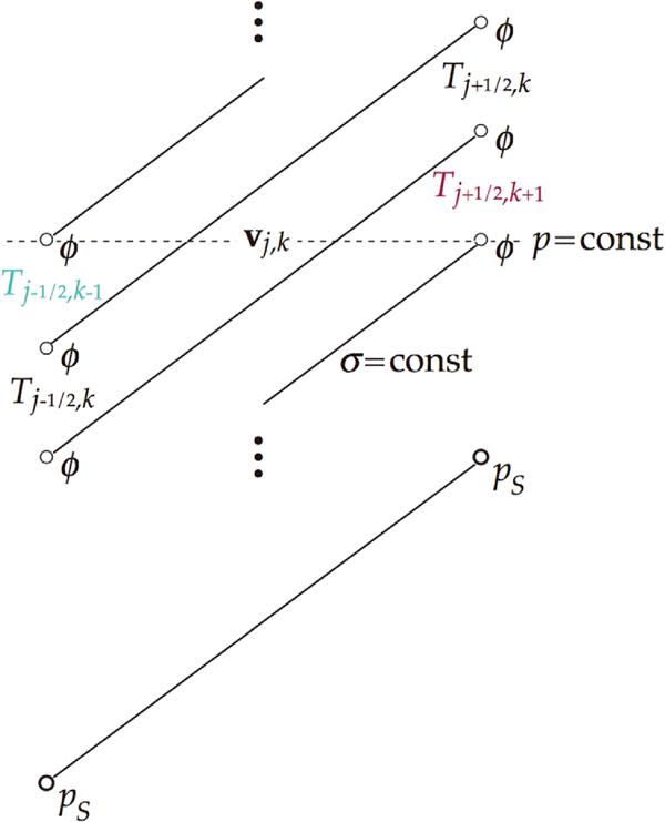
The problem is clearly not one of the truncation error in the vertical, as it is formally defined, since it would be reduced by increased vertical resolution, while the problem just described would only get worse. In that sense an instructive example was presented in Mesinger (1982), reproduced with a correction in Mesinger and Janjić (1985), of errors for two temperature profiles and two schemes as the vertical resolution was increasing. A hydrostatically consistent scheme of the two, that of Burridge and Haseler (1977), fortuitously had zero error for poor vertical resolution to start with, but had an increasing error as the vertical resolution improved. If, on the other hand, both horizontal and vertical resolution were to be increased by the same amount, e.g., doubled, the problem would remain the same.
Hybrid terrain-following vertical coordinates now used in most “production models” (term introduced by Cullen 2007) tend to be of a kind that reduces the imprint of topography with height faster than the original “basic” terrain-following coordinate (BTF, e.g., Klemp 2011). Schär et al. (2002) proposed a scheme which prescribes small-scale topography features to decay with height faster than the larger-scale ones, naming it SLEVE (Smooth Level Vertical) coordinate. This prescription was further refined by Klemp's (2011) smoothed terrain-following (STF) coordinate, allowing for additional smoothing with height while avoiding reduction of the vertical grid spacing below a given minimum. Illustrations of the impact of three of these varieties of terrain-following coordinates, elevation-defined BTF, Simmons and Burridge's (1981) hybrid (HTF) coordinate, and SLEVE, for a chosen real topography are shown in Schär et al. (2002). Illustration of the impact of the three of them and the STF, for an idealized topography, are shown in Klemp (2011). Both Schär et al. (2002) and Klemp (2011) tests confirm advantages of the smoothed coordinates, with the latter in addition suggesting a simplified version of the vertical interpolation method, achieving additional benefits with little computational overhead.
One among “essential or at least highly desirable” properties that Staniforth and Thuburn (2012) suggested dynamical cores should have was that “The geopotential gradient and pressure gradient should produce no unphysical source of vorticity”. Weller and Shahrokhi (2014) independently noted that existing models “do not have curl-free discretizations of the gradient operator, which is likely to lead to problems over steep orography”. Benefiting from the property of covariant velocity components when used on non-orthogonal grids, as customarily done, to enable curl-free calculation of pressure gradients, they performed tests over idealized orography confirming the advantages of the curl-free formulation.
Performance of the curl-free formulation of the pressure gradient was tested by Ujiie and Hotta (2019) aimed to remove the problem of “spectral blocking”, accumulation of power near the truncation limit they had. In grid point models of course Arakawa-type horizontal advection schemes are well known to control the spurious cascade of energy toward smaller scales within the basic two-dimensional nondivergent flow, but as pointed out by Ujiie and Hotta models also contain other nonlinear terms.
3. Non-conforming grid systems: immersed boundary, and cut-cells
While the terrain-following coordinates are defined so as to have their lowest surface follow topography, there are two other topography treatments that do not conform the grid but instead adjust the discretization schemes to accept the topography. One of them keeps the curvilinear two-dimensional shape of the topography as prescribed, and is referred to usually as the immersed boundary method, IBM. The other defines the shape of grid cells to approximate the topography, as felt suitable for the discretization chosen. This would be the step-topography method defining grid cells simply as either land or air, or a cut-cell scheme in which grid cells are cut at angles as defined by the scheme used.
The immersed boundary method, IBM, came into atmospheric applications from engineering, originally addressing a topic as remote from atmosphere as flow around heart valves (Peskin 1972). In Peskin's original design the boundary was represented by point sources distributed so as to constrain the fluid to its irregular domain. Allen and Zerroukat (2019) summarize some features of this design. With it, all the grid points were inside the fluid. A variant of the method dominant today was introduced later by Tseng and Ferziger (2003), with an irregular boundary of “terrain” inside a regular grid consisting of cells. Its essential numerical component consists of marking grid points of cells that include the boundary but are under the terrain, naming them “ghost” points, and reflecting them in the direction normal to the boundary and into the fluid, referring to reflection points as “image” points (Lundquist et al. 2010, and references therein). The values at image points are subsequently obtained by appropriate interpolations using fluid values at surrounding computation points. As different numbers of actual fluid values might be available depending on the specific geometry in place, a variety of interpolation options need to be provided for. Ghost point values can then be related to the obtained image point values to satisfy either a Dirichlet or Neumann boundary condition, as appropriate, thus enabling integration to proceed. An additional feature of the method is that a body force term needs to be added to the momentum equation so that the velocity normal to the boundary decreases to zero when approaching the boundary (Lundquist et al. 2010, 2012; Allen and Zerroukat 2019). See Mittal and Iaccarino (2005) for further references.
Lundquist et al. (2010) following idealized tests of IBM implemented in a nested fashion as IBM-WRF, pointed out WRF's ability to provide synoptic-scale forcing for IBM handling of complex urban terrain. They developed modifications of the WRF physics parameterizations to account for the effects of the immersed terrain. This included implementing a no-slip boundary condition common in CFD simulations of complex topography such as urban landscape. In Lundquist et al. (2012) they reported on a three-dimensional extension of the method, with the inner WRF nest being an Oklahoma City terrain with numerous explicitly resolved urban buildings. Bao et al. (2018) further extended this, now referred to as WRF-IBM system, to accommodate the use of several neutral stability options of the Monin-Obukhov theory, and taking into account the difference between the vertical gradient standard in atmospheric surface layer parameterizations and the surface-normal gradient appropriate for IBM. Numerous other WRF-IBM boundary physics refinements are summarized and/or cited in Bao et al. (2018), and validations for field campaigns over a moderately sloped Askervein Hill and a steeply sloped Bolund Hill are presented.
In addition to physics modifications, issues that also need attention arise related to the numerical framework of the parent atmospheric model (e.g., Allen and Zerroukat 2018, 2019, among others). Here we refer to “parent” model as one in which IBM numerics was implemented, along with physics refinements, as opposed to the usage of the term in limited area NWP and regional climate studies, where the term refers to the model generating lateral boundary conditions. Numerous atmospheric IBM tests, on the other hand, address specific much smaller scale application purposes.
WRF-IBM's performance in these various tests offers convincing evidence that a powerful tool has been generated for complex terrain applications and studies, such as urban dispersion, wind energy, impact of possible development projects, aimed, e.g., to movement in the direction of “green cities”, and the like. Scales addressed are those of large-eddy simulations or something similar, with horizontal grid distances of 5 m and less. While atmospheric prediction models aim for increasingly higher resolutions, the highest resolutions attained at the time of this writing are far coarser, at most a kilometer or somewhat less. The most typical of the highest resolutions explored might be Vionnet et al. (2015), including tests at 0.25 km resolution. In addition to filtering two grid increment orography features at all their resolutions, at 0.25 km Vionnet et al. (2015) needed a local filter to remove slopes higher than 45°. While IBM methods at these resolutions could in principle handle topography as is, Arthur et al. (2018) point out that "accuracy of the IBM appears to degrade with coarser grid resolution”. Thus there is as tends to be referred to a “gray zone” of tens to hundreds of meters, where the performance of IBM requires attention. Improving the performance of WRF-IBM at these resolutions, not yet studied extensively, is explored by Arthur et al. (2018) and more recently Arthur et al. (2020).
Another way of addressing the errors of terrain-following systems as the steepness of topography is increased is of course to move away from the terrain-following systems. Motivated by the success of very simple wall-mountains of Egger (1972) this has been done by Mesinger (1984) and implemented at U.S. NWS as a “step-mountain” model, later referred to as the Eta model (Mesinger et al. 1988; Mesinger 2004b). The model used a modification of the sigma coordinate
with
z being the geometric height, and prf (z) being a suitably defined reference pressure as a function of z. Furthermore, since the Eta is a layer model, the ground surface heights zS are prescribed rounded off to a chosen discrete set of values defining the vertical resolution of the model.
Very quickly upon becoming officially an operational NWS model the Eta achieved precipitation skill scores visibly better than those of two sigma system NWS operational models. Thus, in 1998, the Eta 24 h precipitation scores verifying at 48 h lead time were better than those of the NGM/RAFS system verifying at 24 h lead time (Mesinger 2004b). Both models were run at a resolution of 80 km, very coarse by today's standards, and not one at which problems of terrain-following coordinates are generally expected to be serious. Various tests however strongly indicated that the use of coordinate surfaces intersecting topography was a significant reason for this Eta advantage in skill. Placement of centers of major lows was another verification method in which the Eta showed advantage over its NCEP driver global model (e.g., Mesinger and Veljovic 2017, hereafter MV2017).
In spite of these results, discovery of the flow separation problem by Gallus and Klemp (2000), caused by the step corners of the step-topography eta, led numerous authors to believe that the eta coordinate system is “ill suited for high resolution prediction models”. Mesinger (2004b) lists five citations with this or similar statements, and subsequently there have been more (e.g., Thuburn 2011, among others). Weaknesses of the step-topography eta in two real data studies have been pointed out in a subsequent study by Gallus (2000), recalling also a failure of an experimental 10-km Eta to simulate a case of a Wasatch downslope windstorm, while a sigma system MM5 performed well (Staudenmaier and Mittelstadt 1997). Accordingly, when developing an 8-km NMM (Nonhydrostatic Mesoscale Model), based on the Eta, NCEP in 2002 decided to use a terrain-following coordinate, with an announcement that “This choice [of the vertical coordinate] will avoid the problems … with strong downslope winds and will improve placement of precipitation in mountainous terrain” (Geoff DiMego, personal communication, 19 July 2002).
Nevertheless, when eventually more than four month (January 1 to May 22; hereafter referred to as “our+ month”) “parallel” test was run comparing the performance of the Eta vs. NMM the placement of precipitation by the Eta was clearly better (MV2017, Fig. 4). Both models were coupled to their own data assimilation systems where the NMM used the GSI which was more advanced than the EDAS used by the Eta. It is noteworthy that the advantage of the Eta was increasing with longer lead times, as the models moved away from their different data assimilation systems, becoming particularly prominent at 72 h and at 84 h verification times; and also for more intense precipitation thresholds, of 0.5 inch (24 h)−1 (i.e., 12 mm (24 h)−1) and higher. One should also note that the Eta advantage came predominantly from the mountainous western United States (DiMego 2006), where the choice of the terrain-following vs. terrain intersecting coordinate system of the two models would be expected to have the most impact.
The Gallus and Klemp (2000) flow separation problem of the step-topography Eta was addressed by refining the eta discretization so as to define piecewise linear sloping bottoms of velocity cells. This was done by checking values of topography boxes centered at corners of the velocity cell, and prescribing the bottom elevation to linearly decrease one layer thickness from either the highest or the two neighboring highest values in the directions of the remaining three or two cell corners. Thereby step corners responsible for the Gallus-Klemp flow separation problem are eliminated. Indeed, once a code problem was noticed and addressed, simulation of the Witch of Agnesi test gave a comparable and perhaps slightly more accurate result than that of Gallus and Klemp (2000) following artificial modification of their step-topography code to address the problem (MV2017).
With the bottom slopes of this Eta cut-cell scheme extending only one step in the horizontal and one layer thickness in the vertical there are no small cell problems. Generalization of the scheme to admit slopes across two steps, and within depths of two layers, is straightforward and planned as a future task.
The more common height coordinate version of cut-cell schemes introduced by Adcroft et al. (1997) for an ocean model, then referred to as “shaved cells”, also has height of the model terrain prescribed at corners of the cell; but the topography surfaces of cells are prescribed to take terrain values at all four vertices of the cell column. Thus, various cell volumes can be created, and rules must be prescribed to restrict cell volumes from being too small. A somewhat simplified version of the scheme was implemented in a C-grid atmospheric model by Steppeler et al. (2002), demonstrating a successful simulation of flow over the Witch of Agnesi topography. Subsequently, Steppeler et al. (2006) evaluated 24-h forecast skill of 39 real-data cases over European domains using resolutions of 7 km and 14 km, and reported on a “rather systematic improvement of precipitation forecasts” compared to the terrain-following version of the model. In Steppeler et al. (2013) a set of six five-day forecasts was analyzed choosing a model area centered southeast of the Himalayas, finding that the cut-cell model improved the precipitation forecasts compared to a control model “everywhere by a large margin”. Finally, in Steppeler et al. (2019) results of six 10-day forecasts of the positions of Atlantic lows in the lee of the high orography of Greenland were studied using a terrain-following and a cut-cell model versions. The position errors using the cut-cells were found to be smaller or equal to those using the terrain-following version.
These real data tests have been complemented by a number of idealized studies. Yamazaki and Satomura (2008, 2010) reported on successful results over a wide range of slopes and studied cell-combining approaches vertically or horizontally aimed at eliminating small cells. Lock et al. (2012) studying idealized cases report on “smooth results near the lower boundary, even for a relatively coarse vertical resolution”. They do however point out the complexity of the method as used, admitting 79 possible orientations of the cut-cells. Good et al. (2013) performed tests of the cut-cell method in three idealized cases, and comparing results with those of terrain-following models find the errors associated with terrain-following coordinates reduced or even greatly reduced by the cut-cell approach. Shaw and Weller (2016), on the other hand, report on results contradicting those, as well as the earlier tests of Schär et al. (2002), and Klemp (2011). They ran several standard tests and also three newly designed ones, and pointing out their having used a single model, find no significant advantage of cut cells or smoothed coordinates over a traditional terrain-following system.
Many authors suggest that non-conforming grid systems, those not terrain-following, have parameterization challenges because of their coarse resolutions above high topography (e.g., Chow et al. 2019, among others). As a remedy, Yamazaki and Satomura (2012), and Yamazaki et al. (2016), propose and test use of locally refined grids, common in engineering applications, in atmospheric tests referred to earlier as block-structured mesh by Jablonowski et al. (2006, 2009). We are however not aware of any tests of the seriousness of errors addressed, those errors depending of course on how refined the model boundary layer and turbulence schemes are.
Regarding this issue, in the four+ month “parallel” test, comparing the NCEP Eta system against the NMM/GSI, with very similar boundary layer and turbulence closure schemes of the two but very different vertical resolutions in the boundary layer, a result was obtained just the opposite of the referred to expectations. The two models had 60 vertical layers each, but NMM used the sigma system from the ground up to 420 hPa, with the lowest layer about 40 m at sea level deep and thickness in pressure decreasing upwards; while the Eta starting at about 20 m at sea level in the lower troposphere had layer thicknesses in pressure that increased with height (DiMego 2006, slides 10 and 11). With these setups, in the Continental U.S. (ConUS) West area (DiMego 2006, slide 51), including most of the US Great Plains, at elevations of about a mile layer thicknesses of the NMM reduce to less than 35 m, while those of the Eta increase to more than 150 m. Yet, as shown in Fig. 2, where NAM stands for the operational Eta/EDAS, NAMX for NMM/GSI, and OBS for observations, over the ConUS West 10-m winds of the Eta were more accurate than those of the NMM (from DiMego 2006, slide 65). In the plots of the figure, twice daily forecasts January-May 2006, at 12-km resolution, are verified by NCEP “Forecast Verification System”. See DiMego (2006) for additional details, and Mesinger et al. (2012) along with Mesinger (2010) for the summary of the Eta boundary layer and turbulence schemes in place.
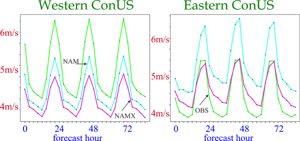
We see no obvious explanation for the Eta 10-m skill with its thicker layers over the U.S. West being better than that of the NMM. Of the NMM boundary layer code changes listed in DiMego (2006) one that perhaps stands out is the replacement of the wind direction dependent form drag scheme of the Eta of Mesinger et al. (1996) by a more conventional prescription of roughness length, z0, depending on subgrid terrain variability and vegetation type. But with more than 300 forecasts verified in Fig. 2, and the NMM system having been planned as a replacement of the Eta for several years prior to the results of Fig. 2, receiving during that time all possible development efforts compared to the Eta being mostly “frozen”, we see the left-hand plot of Fig. 2 deserving attention. We find it reasonable that large horizontal gradients of volumes of NMM cells across high topography of the Rockies vs. not much cell volume change with the terrain-intersecting coordinates of the Eta should favor Eta in view of the conservation properties of the Arakawa horizontal advection schemes (Janjić 1984) in place in the two models. Note that these conservations are accomplished via exchanges between pairs of cells neighboring each other along the surfaces of constant sigma and/or eta.
Attention to errors of terrain-following coordinates by various authors was on the other hand motivated primarily by errors of horizontal discretization resulting from increased slopes of coordinate surfaces as model resolutions are increased. These can be addressed by vertical interpolation, following Kurihara (1968), Mahrer (1984), Klemp (2011), Zängl (2012), and others, but there is little evidence if that achieves improvements comparable to those reported by Steppeler et al. (2006, 2013), by Section 2 of MV2017, and those of the left-hand plot of the present Fig. 2. Some of the improvements are accomplished at resolutions at which steepness of model topography could not have been all that high. Note considerable benefits reported by Russell (2007) from a terrain-intersecting as opposed to a terrain-following choice at climate sensitivity resolutions, implemented later in experiments aimed at projections of changes resulting from successive doublings of CO2 (Hansen et al. 2013). If the steepness of model orography were the basic driver of advantages of terrain-intersecting over the terrain-following systems, then those advantages should be very small when addressing large scales and not using particularly high resolutions.
With these points in mind, we feel it should be useful to recall and expand on the results of the MV2017 ensemble experiment in which the limited area, cut-cell Eta model, driven by ECMWF (hereafter EC) 32-day ensemble members, achieved improved accuracy of large scales for an extended period compared to that of its driver members. This is the subject of our next section.
4. Cut-cell Eta large scale skill vs. ECMWF
While here we are focused on representation of topography, behavior of codes for phenomena for which resolution should not be a problem deserves interest beyond just topography. This is because when significant differences in code performance are identified in spite of resolution not being an issue, it makes sense to try to understand why. With this in mind we have in MV2017 addressed verification of large scales known of dominant interest for weather, the tropospheric jet stream.
Driving a limited area model (LAM) by LBCs from a global model, can one improve on the largest scales? MV2017 points out four requirements that need to be fulfilled by a LAM, be it in Regional Climate Modeling (RCM) or NWP environment, to improve on large scales inside its domain, as follows.
First, an RCM/NWP model obviously needs to be run on a relatively large domain. Note that the domain size, in terms of computational cost, is relatively inexpensive compared to resolution. Namely, doubling the domain size, in each direction, vs. doubling the resolution, increases computational cost by a factor of 4, vs. the increase by the factor of 8, respectively.
Second, the RCM/NWP model should not use more forcing at its lateral boundaries than required by the basic mathematics of the problem. That means prescribing lateral boundary conditions only at its outside boundary, with one less prognostic variable prescribed at the outflow than at the inflow parts of the boundary.
Next, nudging towards the large scales of the driver model must not be used, as it would be nudging in the wrong direction if the nested model can improve on large scales inside its domain.
Finally, the RCM/NWP model must have features that enable development of large scales that are improved compared to those of the driver model. When such improvement is seen it would typically be expected to come from higher resolution, but obviously does not have to.
The first convincing demonstration of an improvement in large scales by an RCM compared to those of its driver global model may have been that of Fennessy and Altshuler, presented in 2002 at an AGU meeting, and reported quite a few years later in Veljovic et al. (2010). Here we summarize and extend the results of MV2017 who demonstrated in an ensemble experiment, driving cut cell Eta by EC 32-day ensemble members, an advantage of the Eta for a period of a week or so in the accuracy of large scales, as represented by 250 hPa winds. We shall illustrate these improvements in a number of ways, aiming to enlighten as best we can how this presumably generally unexpected result could have taken place.
Needless to say, in the MV2017 Eta ensemble the first three requirements above have been fulfilled, as not doing so regarding any one of them would have meant working against the objective of improving on large scales. As to the fourth one, the driven LAM required to have features enabling improved accuracy of large scales, one should note that during the first 10 days of the experiment the resolutions of the two ensembles were about the same. Still, it was precisely during that time that a convincing advantage of the Eta was achieved. With the resolution thus being removed from possible reasons for the Eta advantage, determining other causes is obviously a matter of considerable interest.
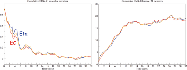
Two verification scores were used in MV2017 to inspect the model skill in forecasting large scales: the ETS or Gilbert skill score corrected to unit bias, ETSa (Mesinger 2008; Brill and Mesinger 2009) for wind speeds > 45 m s−1, and the RMS difference, both at 250 hPa and compared to EC analyses. The purpose of the correction to unit bias of the ETS or Gilbert score is to have a verification of the position of the variable forecast. While the RMS difference measures the skill of forecast winds at all speeds, it seems reasonable that the RMS difference will be dominated by differences at large scales.
Given that there is considerable evidence of the benefit the Eta model derives from its use of the eta coordinate, and for a test of this benefit in a larger ensemble sample, MV2017 have rerun their 21 member Eta ensemble by having the Eta switched to use sigma, hereafter called Eta/sigma. The two scores of the driver EC ensemble, the Eta, and the Eta/sigma, are reproduced here in Fig. 3.
A conspicuous feature of the scores shown is the considerable advantage of the Eta (blue) over the EC (red) during about day 2–6 of the experiment. This happens to be the time when a major upper-tropospheric trough was crossing the Rockies (MV2017, Fig. 10), a situation in which various NWP results of the operational Eta showed advantage over sigma system models run at the time at NCEP (MV2017, Section 2).
We are somewhat puzzled however by the Eta/sigma (orange) having demonstrated a visible advantage over the EC during this time as well; and in addition an advantage comparable to that of the Eta later at day 7–10 time. Days 12–13 and 16–19 could be added to this list, although with some restraint given that at these times the skill of all models is rather low. We show more results and comment on possible reasons behind this Eta and also Eta/sigma skill in the following subsections.
4.1 Illustration: 250 hPa wind speed plots
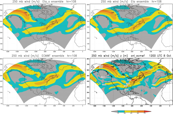
To complement the numerical information of Fig. 3 on scores achieved, in Fig. 4 we show 250 hPa wind speed averages for all 21 members, at day 4.5. See figure legend for the content of its panels.
While predicting the major pattern, EC members, bottom left, do not extend the > 45 m s−1 jet streak entering Alaska sufficiently southeastward, and have the streak across contiguous U.S. and off New England too far westward. These features are improved on Eta/sigma and Eta maps, top left and top right, respectively, in particular by the Eta in terms of covering a bit of eastern Labrador, and more of the ocean area off the U.S. New England states and toward the tip of Greenland.
It is interesting to note that the advantage of the Eta over Eta/sigma as seen on these average maps seems to come just about entirely from the better placement of the streak of > 45 m s−1 over contiguous U.S. and off to northwestern Atlantic, and not from the streak entering the model domain over northern Alaska. We suspect this could be because of the former feature having had to cross the major Rocky Mountains topographic barrier, as opposed to the latter having entered the North American continent at lower elevations northeast of the Rockies.
4.2 Verification via the number of “wins”, according to ETSa, RMS, and SEDS scores
The advantage of the Eta over the EC is demonstrated perhaps to even a greater degree by the number of “wins” of one model vs. another. Thus, in Fig. 5, left panel, the number of wins of the Eta 250 hPa winds > 45 m s−1 and its EC driver members vs. each other are shown as a function of time, according to our score that verifies the accuracy of the placement of the variable verified using the Equitable Threat (or Gilbert) Score adjusted to unit bias (ETSa). Same, but according to the RMS difference of the forecast and analyzed winds, and for all winds at 250 hPa, is shown in the right panel.
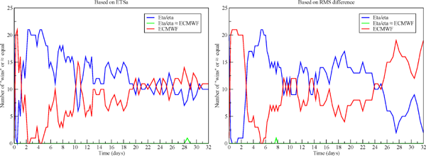
Initially the EC members have an advantage, presumably due to errors the Eta members absorb as a result of initializations off their EC driver members. The advantage of the Eta later on is particularly striking in the ETSa scores of days 2 to 6, with four verifications in which all 21 Eta members have better scores of the placement of strongest winds than their EC driver members. But according to both scores the Eta members are more accurate during most of the first 20 days or so.
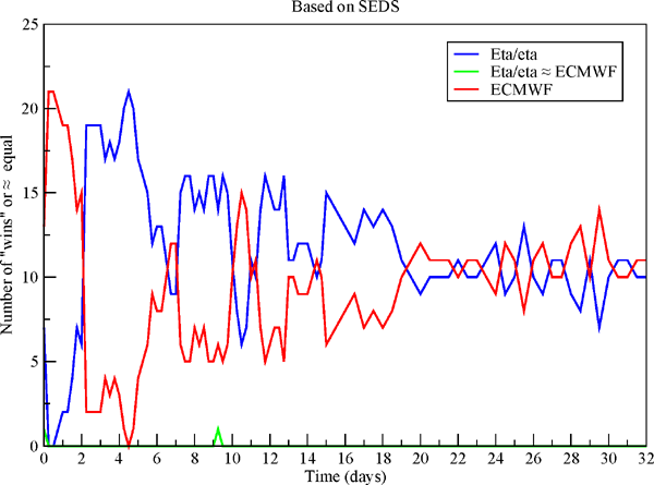
Given that we wish to emphasize the placement accuracy of strongest winds and that the score we chose to that end, ETSa, is not widely used, we use here yet another measure to compare the skill in that sense, “symmetric extreme dependency score” (SEDS), proposed by Hogan et al. (2009; see also Wilks 2011). As pointed out by Hogan and Mason (2012) SEDS is asymptotically equitable (Gandin and Murphy 1992; Wilks 2011), asymptotically referring to the limit as sample size is increasing; and not trivial to hedge. Removal of the impact of hedging via bias different from one was precisely the objective of adjusting the ETS to unit bias by the assumption introduced in Mesinger (2008). Note that just as with the ETSa, a higher value of SEDS is better, and the perfect value is one.
“Wins” of the two models, Eta and the EC, vs. each other, according to the SEDS values as a function of time, are shown in Fig. 6. Very similar to plots of Fig. 5, dominance of the Eta is seen during days 2–6, with all 21 Eta members at day 4.5 having better scores than their EC driver members. Note that at this time the ETSa scores, Fig. 5 left panel, also show all 21 Eta members having higher scores than their EC driver members. At later times, just as in the two plots of Fig. 5, the Eta members display better SEDS scores most of the time until around day 20 of the experiment.
4.3 Skill of the Eta/sigma vs. the EC according to the number of wins
Recalling the results of the Eta/sigma of Fig. 3, an obvious question is if the Eta/sigma achieves similar advantage over the EC if scores are compared according to the number of wins. The number of wins of the two models, Eta/sigma vs. the EC, using the three scores of the preceding subsection, are shown in Fig. 7.
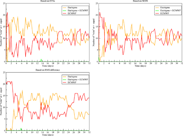
The advantage of the Eta/sigma over the EC during the first 10 days, when the resolution of the two was about the same, is confirmed by the scores of the top left plot of Fig. 7. As in Fig. 3, this advantage is reduced compared to that of the Eta, with at most 19 Eta/sigma members showing better scores than the EC, never all 21, and never 20. One can however notice that the advantage of the Eta/sigma during days 2–6, the time of the upper-tropospheric trough crossing the Rockies, does not stand out as it did for the Eta. It is in fact rather comparable with that of the latest part of the first 10 days, days 7–10. The advantage of the Eta/sigma the next about 10 days, when the resolution of the EC was reduced and that of the Eta/sigma just as that of the Eta was not, suggests that the reduced resolution of the EC did not have much impact on scores we are inspecting.
The next two plots of Fig. 7 even to a stronger degree confirm the disappearance of the Eta's extraordinary dominance over the EC seen in Fig. 3 and in the left-hand plot of Fig. 5, during days 2–6 of the experiment. Altogether, the three plots of Fig. 7 we see as offering convincing support for the synoptic situation of days 2–6, specifically that of the upper-tropospheric trough crossing a major topographic barrier, as being the main cause of the Eta large scale skill advantage over the EC during that time. Note that this only adds additional evidence to results of experiments and comparisons to other sigma system NCEP operational models summarized in Section 2 of MV2017.
4.4 Eta vs. Eta/sigma in terms of number of wins
With the results we have at hand we can compare in terms of the number of wins the remaining pair of models, Eta and the Eta/sigma. The number of wins of these two models according to the same three skill measures as used for the preceding figure is shown in Fig. 8.
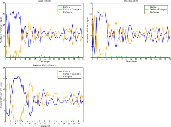
The three plots of Fig. 8 strongly confirm the dominance of the Eta over the Eta/sigma during the referred to time of the upper-tropospheric trough crossing the Rockies, days 2–6. Using the three skill measures, ETSa, RMS, and SEDS all 21 Eta members in that time achieve better scores than their corresponding Eta/sigma members 7, 3, and once more 7 times, respectively. Following that period and approaching day 10 the Eta/sigma shows an advantage during a short period of about a day or two. This signal, although not as very strong, is seen also in the two plots of Fig. 3. We have at present no candidate reason for this advantage of the Eta/sigma, but hope to return to this issue at a later time. Advantage of the Eta for several consecutive verifications according to all three scores is seen again later around days 15–16, but certainly once the model skill becomes quite small the results deserve less attention than those at earlier lead times.
4.5 Verifications using contour plots
Focusing here mostly on the placement of areas of the strongest winds representing speeds > 45 m s−1, we wish next to inspect how the models have placed these areas compared to verification. Thus in the upper panel of Fig. 9 in yellow-brown we show contours of the 250 hPa wind speeds of 45 m s−1 of the 21 EC driver members at 4.5 day lead time along with verification in red. We chose the 4.5 day lead time because it is the longest of the 4 verification times with all 21 Eta members winning the ETSa scores against their EC drivers. In the middle panel we show the same, but for the 21 Eta members; and in the lower panel the same, but for the Eta/sigma members.
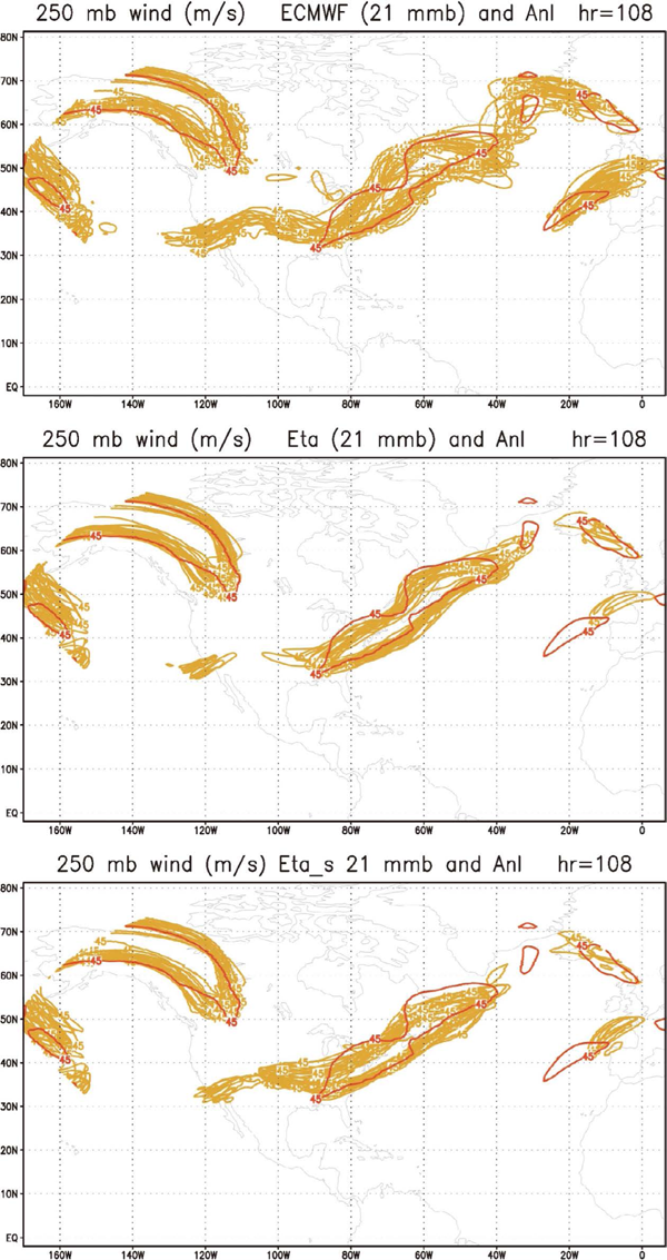
While the contours of various jet streaks generated by the EC members, upper panel, are generally in the right places, tendencies to include some areas which did not verify are present as well. In particular, numerous contours erroneously extend across the central and southern United States all the way into the eastern Pacific. Another feature that did not verify is the coverage by many if not all EC contours over a considerable part of the Labrador peninsula, bulging to the northwest into it as opposed to just the opposite of the analysis contour. An area of excessive coverage is perhaps also present over southeastern Greenland and to the east, once again over a region mostly in the lee of high topography.
The first two of these weaknesses are almost completely absent in the Eta ensemble contours, middle panel. This in particular refers to the lack of contours extending from the central United States into the high elevation area of the Rockies, and to no contours bulging into the Labrador peninsula—all of them instead reproducing the concave shape of the analysis contour. As to the area further to the east, the lack of extensive coverage seen east of Greenland might be due to the absence of stochastic physics in the Eta but used by the EC now for a long time (Buizza et al. 1999; Palmer et al. 2009, among others).
Contours of the Eta/sigma ensemble, bottom panel, regarding the first feature above are also improved compared to the EC contours, but do contain many members extending across the central United States—a few of them all the way to the eastern Pacific. Thus, some of this EC error is reintroduced. In the area of southern Labrador and further to the northeast the Eta/sigma contours, somewhat similar to those of the Eta, cover much less unverified area than those of the EC, but fail to maintain the concave shape of the Eta contours across southern Labrador. Instead, the northeastern part of the jet streak contours east of Labrador, is shifted southward by the Eta/sigma in disagreement with the analysis. But overall, compared to the EC contour map, the contour positions of the Eta/sigma are certainly still an improvement. Determining the features of the Eta that should be credited for this improvement, just as that shown in the plots of scores of days 2 to 10, and in the top left map of Fig. 4, is difficult. We shall return to this issue in our concluding section.
5. Discussion and comments
While in numerous reports on advances in global NWP and climate models stability problems are encountered as the model resolution increases and model topographies become steeper, nevertheless terrain-following systems of various hybrid flavors dominate. Vertical interpolation of the pressure gradient force is one remedy in use. Thus, of seven models covered in a recent review of global cloud-resolving models (Satoh et al. 2019), only one is not using a terrain-following system, but a “box-fill method” instead, presumably a step-topography scheme. Among other major systems GEM from Environment and Climate Change Canada, is changing from pressure based to a height based system, motivated by efficiency including that due to the pressure gradient when using unchanging stencil (Husain et al. 2019).
Of alternative systems, most current efforts are apparently devoted to the immersed boundary method. Impressive results have been reported, as cited and many more, addressing topographies including sections of metropolitan cities with building sides that cannot be handled using terrain-following systems. The method has been implemented within the WRF model, with adjustments to its boundary layer parameterization schemes, for use in various studies. Applications such as in air quality, heating, city and transport development, etc., are obviously numerous and of the highest economic and health values.
While use of the IBM in atmospheric NWP models is an option that has been investigated with domains not permitting resolutions as fine as that needed for LES scales, e.g., Arthur et al. (2018), to our knowledge it has not been successful so far. Step-topography and cut-cell methods on the other hand as summarized have been demonstrated performing better than the terrain-following schemes in a number of NWP types of tests.
Several “gray zone” resolution idealized tests have suggested the cut-cell to be advantageous when comparing cut-cell vs. terrain-following options with grid increment distances greater than those of LES up to some hundreds of meters. An exception are tests of Shaw and Weller (2016) who find “no significant advantages of cut cells or smoothed coordinates” when using a single model. Clearly, additional studies are desirable.
Another obvious option is the use of the IBM scheme in a limited domain, in combination with another more standard topography scheme in a larger “driver model” domain (e.g., Lundquist et al. 2010; Allen and Zerroukat 2019). An issue deserving attention though is that IBM schemes as summarized use interpolation procedures to impose boundary conditions at the terrain surface, which is not compatible with finite-volume methods. This would be a limitation in view of a number of properties perhaps generally considered that dynamical cores of NWP and climate models should have (e.g., Staniforth and Thuburn 2012; but note also Peixoto 2016).
Results we present and discuss in Section 4 addressing our earlier experiment, reported in MV2017, with the cut-cell Eta and also Eta/sigma driven by EC ensemble members, suggest two key points we feel deserve attention beyond our focus on representation of topography.
First, our experiment demonstrates that running a LAM such as an RCM, driven by a global model, improvement of large scales of the driver model is possible. While, as stated by Davies (2017) “In NWP, it is widely recognized that LAM skill is greater when domain size is increased”, there are very few efforts in various RCM and LAM studies in that direction.
Acceptance of the possibility of improving on large scales inside the LAM domain contradicts two widespread paradigms of RCM modeling: use of the Davies' relaxation LBC scheme along with a buffer zone around the RCM boundary (Davies 1976), and of performing large scale or spectral nudging inside the RCM domain. The former of these, relaxation, seems to be used with hardly any exceptions (e.g., Giorgi 2019; Table 1 in Tapiador et al. 2020), even though it is in conflict with the fundamental mathematical nature of the equations we are solving. The latter, large scale or spectral nudging, while often used, “opinion” on its “usefulness … has varied” (Giorgi 2019). With some groups however, the belief in spectral nudging appears to be very firm, even though it suffers from the same conflict as the relaxation. Note the title of Omrani et al. (2012), and the topic addressed by Schaaf et al. (2017).
The improved skill shown in running the limited area Eta model without using resolution higher than the driver EC model the first 10 days raises our second key point that the Eta model dynamical core presumably must contain features responsible for the improvements achieved. It seems to us far from likely that the Eta physics is critically impacting 250 hPa winds in the lee of topography. In addition, we are not dealing with improvements compared to a substandard model. Note the words of the recent review of numerical methods by Côté et al. (2015), “Although spectral transform methods are being predicted to be phased out, the current spectral model at the European Centre for Medium-Range Weather Forecasts … is the benchmark to beat, and it is not clear that any of the new developments are ready to replace it”.
We feel we have provided convincing evidence that the cut-cell Eta, with about the same resolution as the EC, achieves higher accuracy in forecasting the position of the strongest 250 hPa winds when an upper-tropospheric trough crosses the Rocky Mountains topographic barrier. Using each of three verification scores, we obtained verifications with all 21 Eta members having better scores than their EC driver members. Plots of average winds of the two ensembles and the areas with speeds greater than 45 m s−1 at 4.5 day lead time of our experiment confirm this advantage.
Having available the same ensemble except for the Eta switched to use sigma, i.e., Eta/sigma, we have in addition done all of these tests for two additional pairs of ensembles, Eta/sigma vs. EC, and Eta vs. Eta/sigma. In all of these tests Eta/sigma also shows an advantage over the EC but to a smaller extent. Still, we find the advantage of the Eta/sigma over the EC to be convincing as well particularly in the placement of speeds greater than 45 m s−1 shown in Fig. 4, in the ETSa scores of Fig. 7, and in the contour plots of Fig. 9. In our two remaining scores, RMS and SEDS, an advantage before day 5 is not seen, but a general advantage is strongly indicated later on for a while.
Recall Shaw and Weller (2016) emphasizing their tests of the vertical coordinate in idealized experiments being single model tests. Comparison of the Eta vs. Eta/sigma in our single model test suggests a very decisive impact of the choice of the representation of topography during the time of the upper-tropospheric trough crossing the Rockies. Between the lead time of day 2.00 until and including that of day 5.50, all 21 of the Eta members repeatedly achieve ETSa, RMS, and SEDS scores better than their Eta/sigma counterparts, 7, 3, and another 7 times, respectively. If we were to include verifications of 20 members in those counts, these numbers would increase to about 10 for each score.
One should note that the central subject of the preceding section, namely the impact of the representation of topography on the accuracy of the simulation of the position of upper-tropospheric jet stream winds, addresses an accuracy which seems not measurable by any single verification parameter developed so far. Had such a parameter been available we could have used it to define a null distribution, necessary to arrive at a statistical significance of the conclusions made. We hope that the collection of diagnostics presented instead represents an adequate substitute.
On another point, while the results of the tests of the former pair of ensembles, Eta/sigma compared to the EC, is not the main objective of the present paper, the advantage of the Eta/sigma clearly deserves attention. This is seen in our Fig. 3 and was discussed at some length in our MV2017 reference. Briefly, we feel among the leading candidates responsible for this advantage are our Arakawa horizontal advection scheme (Janjić 1984), finite-volume van Leer type vertical advection of all variables (Mesinger and Jovic 2002), and perhaps also very careful construction of model topography (MV2017), with grid cell values selected between their mean and silhouette values, depending on surrounding values, and no smoothing. Exact conservation of energy in space differencing in transformation between the kinetic and potential energy following Simmons and Burridge (1981) is yet another candidate, given that it is not followed in the EC model, and to our knowledge, not in other production NWP models.
Perhaps an appropriate concluding message of the results presented in our Section 4 might be that the relatively simple scheme of the cut-cell Eta apparently offers prospects of achieving a significant advantage over the almost universally used terrain-following systems of various flavors in present NWP and climate models.
Acknowledgments
In refining the step-topography eta code to make it a cut-cell scheme essential assistance was received from Dušan Jović, then of the Abdus Salam International Centre for Theoretical Physics, Trieste, Italy, and of Jorge Luis Gomes, of the Center for Weather Forecasts and Climate Studies (CPTEC), Cachoeira Paulista, SP, Brazil. In our preparing the summary of the immersed boundary methods kind suggestions of Thomas Allen, of the Met Office, U.K., and help of Fotini Katopodes Chow, and Katherine K. Lundquist, of the University of California, Berkeley, United States, are much appreciated. Our heartfelt thanks go to Thomas L. Black, of the NCEP Environmental Modeling Center, College Park, Maryland, United States, for his dedicated help in raising the level of our manuscript's English to its present state. Finally, we are grateful to two anonymous reviewers, and members of the JMSJ Editorial Board, for comments and suggestions that have been essential for our arriving at the present version of the paper. Our work has partially been supported by the Serbian Academy of Sciences and Arts, via grant F-147, and that of Katarina Veljovic by the Ministry of Science and Technological Development of the Republic of Serbia, under Grant No. 176013.
References
- Adcroft, A., C. Hill, and J. Marshall, 1997: Representation of topography by shaved cells in a height coordinate ocean model. Mon. Wea. Rev., 125, 2293-2315.
- Allen, T., 2007: Comparison of iterative pressure solvers for turbulent flow over hills. Atmos. Sci. Lett., 8, 21-28.
- Allen, T., and M. Zerroukat, 2018: A consistent treatment of the boundary layer for atmospheric models. Quart. J. Roy. Meteor. Soc., 144, 2156-2164.
- Allen, T., and M. Zerroukat, 2019: A semi-Lagrangian semi-implicit immersed boundary method for atmospheric flow over complex terrain. J. Comput. Phys., 397, 108857, doi:10.1016/j.jcp.2019.07.055.
- Arakawa, A., and V. R. Lamb, 1977: Computational design of the basic dynamical processes of the UCLA general circulation model. Methods in Computational Physics. Chang, J. (ed.), Academic Press, 173-265.
- Arthur, R. S., K. A. Lundquist, and J. Bao, 2018: Evaluating the performance of the immersed boundary method within the grey zone for improved weather forecasts in the HRRR model. Tech. Rep. of Lawrence Livermore National Lab. (LLNL), Livermore, CA, United States, 34 pp.
- Arthur, R. S., K. A. Lundquist, D. J. Wiersema, J. Bao, and F. K. Chow, 2020: Evaluating implementations of the immersed boundary method in the Weather Research and Forecasting model. Mon. Wea. Rev., 148, 2087-2109.
- Bao, J., F. K. Chow, and K. A. Lundquist, 2018: Large-eddy simulation over complex terrain using an improved immersed boundary method in the Weather Research and Forecasting model. Mon. Wea. Rev., 146, 2781-2797.
- Brill, K. F., and F. Mesinger, 2009: Applying a general analytic method for assessing bias sensitivity to bias-adjusted threat and equitable threat scores. Wea. Forecasting, 24, 1748-1754.
- Buizza, R., M. Miller, and T. N. Palmer, 1999: Stochastic representation of model uncertainties in the ECMWF Ensemble Prediction System. Quart. J. Roy. Meteor. Soc., 125, 2887-2908.
- Burridge, D. M., and J. Haseler, 1977: A model for medium rage weather forecasting—Adiabatic formulation. Tech. Rep. of ECMWF, No. 4, 46 pp.
- Chow, F. K., C. Schär, N. Ban, K. A. Lundquist, L. Schlemmer, and X. Shi, 2019: Crossing multiple gray zones in the transition from mesoscale to microscale simulation over complex terrain. Atmosphere, 10, 274, doi:10.3390/atmos10050274.
- Corby, G. A., A. Gilchrist, and R. Newson, 1972: A general circulation model of the atmosphere suitable for long period integrations. Quart. J. Roy. Meteor. Soc., 98, 809-832.
- Côté, J., C. Jablonowski, P. Bauer, and N. Wedi, 2015: Numerical methods of the atmosphere and ocean. Seamless prediction of the Earth system: From minutes to months. World Meteorological Organization, WMONo. 1156, 101-124.
- Cullen, M., 2007: Modelling atmospheric flows. Acta Numer., 16, 67-154.
- Davies, H. C., 1976: A lateral boundary formulation for multi-level prediction models. Quart. J. Roy. Meteor. Soc., 102, 405-418.
- Davies, T., 2017: Dynamical downscaling and variable resolution in limited-area models. Quart. J. Roy. Meteor. Soc., 143, 209-222.
- DiMego, G., 2006: WRF-NMM & GSI Analysis to replace Eta Model & 3DVar in NAM Decision Brief. National Centers for Environmental Prediction, 115 pp. [Available at https://www.emc.ncep.noaa.gov/WRFinNAM/Update_WRF-NMM_replacing_Eta_in_NAM2.pdf.]
- Egger, J., 1972: Incorporation of steep mountains into numerical forecasting models. Tellus, 24, 324-335.
- Gal-Chen, T., and R. C. Somerville, 1975: On the use of a coordinate transformation for the solution of the Navier-Stokes equations. J. Comput. Phys., 17, 209-228.
- Gallus, W. A., Jr., 2000: The impact of step orography on flow in the Eta model: Two contrasting examples. Wea. Forecasting, 15, 630-639.
- Gallus, W. A., Jr., and J. B. Klemp, 2000: Behavior of flow over step orography. Mon. Wea. Rev., 128, 1153-1164.
- Gandin, L. S., and A. H. Murphy, 1992: Equitable scores for categorical forecasts. Mon. Wea. Rev., 120, 361-370.
- Gary, J., 1973: Estimate of truncation error in transformed coordinate, primitive equation atmospheric models. J. Atmos. Sci., 30, 223-233.
- Giorgi, F., 2019: Thirty years of regional climate modeling: Where are we, and where are we going next? J. Geophys. Res.: Atmos., 124, 5696-5723.
- Good, B., A. Gadian, S.-J. Lock, and A. Ross, 2013: Performance of the cut-cell method of representing orography in idealized simulations. Atmos. Sci. Lett., 15, 44-49.
- Hansen, J., P. Kharecha, M. Sato, V. Masson-Delmotte, F. Ackerman, D. Beerling, P. J. Hearty, O. Hoegh-Guldberg, S.-L. Hsu, C. Parmesan, J. Rockstrom, E. J. Rohling, J. Sachs, P. Smith, K. Steffen, L. Van Susteren, K. von Schuckmann, and J. C. Zachos, 2013: Assessing “dangerous climate change”: Required reduction of carbon emissions to protect young people, future generations and nature. PLoS One, 8, e81648, doi:10.1371/journal.pone.0081648.
- Hogan, R. J., and I. B. Mason, 2012: Deterministic forecasts of binary events. Forecast Verification: A Practitioner's Guide in Atmospheric Science. 2nd Edition. Jolliffe, I. T., and D. B. Stephenson (eds.), John Wiley & Sons, Ltd., 31-59.
- Hogan, R. J., E. J. O'Connor, and A. J. Illingworth, 2009: Verification of cloud-fraction forecasts. Quart. J. Roy. Meteor. Soc., 135, 1494-1511.
- Husain, S. Z., C. Girard, A. Qaddouri, and A. Plante, 2019: A new dynamical core of the Global Environmental Multiscale (GEM) model with a height-based terrain-following vertical coordinate. Mon. Wea. Rev., 147, 2555-2578.
- Jablonowski, C., M. Herzog, J. E. Penner, R. C. Oehmke, Q. F. Stout, B. van Leer, and K. G. Powell, 2006: Block-structured adaptive grids on the sphere: Advection experiments. Mon. Wea. Rev., 134, 3691-3713.
- Jablonowski, C., R. C. Oehmke, and Q. F. Stout, 2009: Block-structured adaptive meshes and reduced grids for atmospheric general circulation models. Philos. Trans. Roy. Soc. A, 367, 4497-4522.
- Janjić, Z. I., 1977: Pressure gradient force and advection scheme used for forecasting with steep and small scale topography. Contrib. Atmos. Phys., 50, 186-199.
- Janjić, Z. I., 1984: Non-linear advection schemes and energy cascade on semi-staggered grids. Mon. Wea. Rev., 112, 1234-1245.
- Kasahara, A., 1977: Computational aspects of numerical models for weather prediction and climate simulation. Methods in Computational Physics. Chang, J. (ed.), Academic Press, 1-66.
- Klemp, J., 2011: A terrain-following coordinate with smoothed coordinate surfaces. Mon. Wea. Rev., 139, 2163-2169.
- Kurihara, Y., 1968: Note on finite difference expressions for the hydrostatic relation and pressure gradient force. Mon. Wea. Rev., 96, 654-656.
- Lock, S.-J., H. Bitzer, A. Coals, A. Gadian, and S. Mobbs, 2012: Demonstration of a cut-cell representation of 3D orography for studies of atmospheric flows over very steep hills. Mon. Wea. Rev., 140, 411-424.
- Lundquist, K. A., F. K. Chow, and J. K. Lundquist, 2010: An immersed boundary method for the Weather Research and Forecasting model. Mon. Wea. Rev., 138, 796-817.
- Lundquist, K. A., F. K. Chow, and J. K. Lundquist, 2012: An immersed boundary method enabling large-eddy simulations of flow over complex terrain in the WRF model. Mon. Wea. Rev., 140, 3936-3955.
- Mahrer, Y., 1984: An improved numerical approximation of the horizontal gradients in a terrain-following coordinate system. Mon. Wea. Rev., 112, 918-922.
- Mesinger, F., 1982: On the convergence and error problems of the calculation of the pressure gradient force in sigma coordinate models. Geophys. Astrophys. Fluid Dyn., 19, 105-117.
- Mesinger, F., 1984: A blocking technique for representation of mountains in atmospheric models. Riv. Meteor. Aeronaut., 44, 195-202.
- Mesinger, F., 2004a: The steepness limit to validity of approximation to pressure gradient force: Any signs of an impact? Proceeding of 20th Conf. on Weather Analysis and Forecasting/16th Conf. on Numerical Weather Prediction, 84th AMS Annual Meeting, 11–15 January 2004, Seattle, WA, paper P1.19, 14 pp. [Available at https://ams.confex.com/ams/pdfpapers/71364.pdf.]
- Mesinger, F., 2004b: The Eta model: Design, history, performance, what lessons have we learned? Proceeding of Symp. on the 50th Anniversary of Operational Numerical Weather Prediction, 14–17 June 2004, Univ. of Maryland, College Park, MD. [Available at https://pdfs.semanticscholar.org/1dec/50ddf832e6fa01a71d78a6fde22e1eb0e4f1.pdf.]
- Mesinger, F., 2008: Bias adjusted precipitation threat scores. Adv. Geosci., 16, 137-142.
- Mesinger, F., 2010: Several PBL parameterization lessons arrived at running an NWP model. Intern. Conf. on Planet. Bound. Layer and Climate Change, IOP Conf. Series: Earth and Environ. Sci., 13, 012005, doi:10.1088/1755-1315/13/1/012005.
- Mesinger, F., and Z. I. Janjić, 1985: Problems and numerical methods of the incorporation of mountains in atmospheric models. Large-Scale Computations in Fluid Mechanics, Part 2. Engquist, B. E., S. Osher, and R. C. J. Somerville (eds.), Lect. Appl. Math., Vol. 22, 81-120.
- Mesinger, F., and D. Jovic, 2002: The Eta slope adjustment: Contender for an optimal steepening in a piecewise-linear advection scheme? Comparison tests. NCEP Office Note, No. 439, 30 pp. [Available at https://www.emc.ncep.noaa.gov/officenotes/newernotes/on439.pdf.]
- Mesinger, F., and K. Veljovic, 2017: Eta vs. 2sigma: Review of past results, Gallus-Klemp test, and large-scale wind skill in ensemble experiments. Meteorol. Atmos. Phys., 129, 573-593.
- Mesinger, F., Z. I. Janjić, S. Ničković, D. Gavrilov, and D. G. Deaven, 1988: The step-mountain coordinate: Model description and performance for cases of Alpine lee cyclogenesis and for a case of an Appalachian redevelopment. Mon. Wea. Rev., 116, 1493-1518.
- Mesinger, F., R. L. Wobus, and M. E. Baldwin, 1996: Parameterization of form drag in the Eta model at the National Centers for Environmental Prediction. Proceeding of 11th Conf. on Numerical Weather Prediction, 19–23 August 1996, Norfolk, VA, paper 10B.3, Amer. Meteorol. Soc., 324-326.
- Mesinger, F., S. C. Chou, J. Gomes, D. Jovic, P. Bastos, J. F. Bustamante, L. Lazic, A. A. Lyra, S. Morelli, I. Ristic, and K. Veljovic, 2012: An upgraded version of the Eta model. Meteorol. Atmos. Phys., 116, 63-79.
- Mittal, R., and G. Iaccarino, 2005: Immersed boundary methods. Annu. Rev. Fluid Mech., 37, 239-261.
- Omrani, H., P. Drobinski, and T. Dubos, 2012: Spectral nudging in regional climate modelling: How strongly should we nudge? Quart. J. Roy. Meteor. Soc., 138, 1808-1813.
- Palmer, T. N., R. Buizza, F. Doblas-Reyes, T. Jung, M. Leutbecher, G. J. Shutts, M. Steinheimer, and A. Weisheimer, 2009: Stochastic parametrization and model uncertainty. ECMWF Tech. Memo, No. 598, 44 pp. [Available at https://www.ecmwf.int/sites/default/files/elibrary/2009/11577-stochastic-parametrization-and-model-uncertainty.pdf.]
- Peixoto, P. S., 2016: Accuracy analysis of mimetic finite volume operators on geodesic grids and a consistent alternative. J. Comput. Phys., 310, 127-160.
- Peskin, C., 1972: Flow patterns around heart valves: A numerical method. J. Comput. Phys., 10, 252-271.
- Phillips, N. A., 1957: A coordinate system having some special advantages for numerical forecasting. J. Meteor., 14, 184-185.
- Phillips, N., 1974: Application of Arakawa's energy-conserving layer model to operational numerical weather prediction. U.S. National Meteorological Center, Office Note, No. 104, 41 pp. [Available at https://www.ncep.noaa.gov/officenotes/NOAA-NPMNCEPON-0001/013FD944.pdf.]
- Russell, G. L., 2007: Step-mountain technique applied to an atmospheric C-grid model, or how to improve precipitation near mountains. Mon. Wea. Rev., 135, 4060-4076.
- Sangster, W. E., 1960: A method of representing the horizontal pressure force without reduction of station pressures to sea level. J. Meteor., 17, 166-176.
- Satoh, M., B. Stevens, F. Judt, M. Khairoutdinov, S.-J. Lin, W. M. Putman, and P. Düben, 2019: Global cloud-resolving models. Curr. Climate Change Rep., 5, 172-184.
- Schaaf, B., H. von Storch, and F. Feser, 2017: Does spectral nudging have an effect on dynamical downscaling applied in small regional model domains? Mon. Wea. Rev., 145, 4303-4311.
- Schär, C., D. Leuenberger, O. Fuhrer, D. Lüthi, and C. Girard, 2002: A new terrain-following vertical coordinate formulation for atmospheric prediction models. Mon. Wea. Rev., 130, 2459-2480.
- Shaw, J., and H. Weller, 2016: Comparison of terrain-following and cut-cell grids using a nonhydrostatic model. Mon. Wea. Rev., 144, 2085-2099.
- Shchepetkin, A. F., and J. C. McWilliams, 2003: A method for computing horizontal pressure-gradient force in an oceanic model with a nonaligned vertical coordinate. J. Geophys. Res., 108, 3090, doi:10.1029/2001JC001047.
- Simmons, A. J., and D. M. Burridge, 1981: An energy and angular-momentum conserving vertical finite-difference scheme and hybrid vertical coordinates. Mon. Wea. Rev., 109, 758-766.
- Smagorinsky, J., R. F. Strickler, W. E. Sangster, S. Manabe, J. L. Holloway, and G. D. Hembree, 1967: Prediction experiments with a general circulation model. Proc. Int. Symp. Dynamics Large Scale Atmospheric Processes, June 23–30, 1965, Moscow, USSR, Izdatel'stvo Nauka, Moscow, 70-134.
- Smolarkiewicz, P. K., R. Sharman, J. Weil, S. G. Perry, D. Heist, and G. Bowker, 2007: Building resolving largeeddy simulations and comparison with wind tunnel experiments. J. Comput. Phys., 227, 633-653.
- Staniforth, A., and J. Thuburn, 2012: Horizontal grids for global weather and climate prediction models: A review. Quart. J. Roy. Meteor. Soc., 138, 1-26.
- Staudenmaier, M., Jr., and J. Mittelstadt, 1997: Results of the western region evaluation of the Eta-10 model. Western Region Tech. Attachment, No. 97-18, 12 pp. [Available at https://www.weather.gov/media/wrh/online_publications/TAs/ta9718.pdf.]
- Steppeler, J., H.-W. Bitzer, M. Minotte, and L. Bonaventura, 2002: Nonhydrostatic atmospheric modeling using a z-coordinate representation. Mon. Wea. Rev., 130, 2143-2149.
- Steppeler, J., H. W. Bitzer, Z. Janjic, U. Schättler, P. Prohl, U. Gjertsen, L. Torrisi, J. Parfinievicz, E. Avgoustoglou, and U. Damrath, 2006: Prediction of clouds and rain using a z-coordinate nonhydrostatic model. Mon. Wea. Rev., 134, 3625-3643.
- Steppeler, J., S.-H. Park, and A. Dobler, 2013: Forecasts covering one month using a cut-cell model. Geosci. Model Dev., 6, 875-882.
- Steppeler, J., J. Li, I. M. Navon, F. Fang, and Z. Xiao, 2019: Medium range forecasts using cut-cells: A sensitivity study. Meteor. Atmos. Phys., 132, 171-179.
- Tapiador, F. J., A. Navarro, R. Moreno, J. L. Sánchez, and E. García-Ortega, 2020: Regional climate models: 30 years of dynamical downscaling. Atmos. Res., 235, 104785, doi:10.1016/j.atmosres.2019.104785.
- Teixeira, M. A. C., 2014: The physics of orographic gravity wave drag. Front. Phys., 2, 43, doi:10.3389/fphy.2014.00043.
- Thuburn, J., 2011: Vertical discretization: Some basic ideas. Numerical Techniques for Global Atmospheric Models. Lauritzen, P. H., C. Jablonowski, M. A. Taylor, R. D. Nair (eds.), Springer, 59-74.
- Tomine, K., and S. Abe, 1982: A trial to reduce truncation errors of the pressure gradient force in the sigma coordinate systems. J. Meteor. Soc. Japan, 60, 709-716.
- Tseng, Y., and J. H. Ferziger, 2003: A ghost-cell immersed boundary method for flow in complex geometry. J. Comput. Phys., 192, 593-623.
- Ujiie, M., and D. Hotta, 2019: Elimination of spectral blocking by ensuring rotation-free property of discretised pressure gradient within a spectral semi-implicit semi-Lagrangian global atmospheric model. Quart. J. Roy. Meteor. Soc., 145, 3351-3358.
- Veljovic, K., B. Rajkovic, M. J. Fennessy, E. L. Altshuler, and F. Mesinger, 2010: Regional climate modeling: Should one attempt improving on the large scales? Lateral boundary condition scheme: Any impact? Meteor. Z., 19, 237-246.
- Vionnet, V., S. Bélair, C. Girard, and A. Plante, 2015: Winter-time subkilometer numerical forecasts of near-surface variables in the Canadian Rocky Mountains. Mon. Wea. Rev., 143, 666-686.
- Weller, H., and A. Shahrokhi, 2014: Curl-free pressure gradients over orography in a solution of the fully compressible Euler equations with implicit treatment of acoustic and gravity waves. Mon. Wea. Rev., 142, 4439-4457.
- Wilks, D. S., 2011: Statistical Methods in the Atmospheric Sciences. 3rd Edition. Elsevier, 676 pp.
- Yamazaki, H., and T. Satomura, 2008: Vertically combined shaved cell method in a z-coordinate nonhydrostatic atmospheric model. Atmos. Sci. Lett., 9, 171-175.
- Yamazaki, H., and T. Satomura, 2010: Nonhydrostatic atmospheric modeling using a combined Cartesian grid. Mon. Wea. Rev., 138, 3932-3945.
- Yamazaki, H., and T. Satomura, 2012: Non-hydrostatic atmospheric cut cell model on a block-structured mesh. Atmos. Sci. Lett., 13, 29-35.
- Yamazaki, H., T. Satomura, and N. Nikiforakis, 2016: 3D cut-cell modelling for high-resolution atmospheric simulations. Quart. J. Roy. Meteor. Soc., 142, 1335-1350.
- Zängl, G., 2012: Extending the numerical stability limit of terrain-following coordinate models over steep slopes. Mon. Wea. Rev., 140, 3722-3733.