Tailored Ensemble Prediction Systems: Application of Seamless Scale Bred Vectors

Abstract

Uncertainty in numerical weather forecasts arising from an imperfect knowledge of the initial condition of the atmospheric system and the discrete modeling of physical processes is addressed with ensemble prediction systems. The breeding method allows the creation of initial condition perturbations in a simple and computationally inexpensive way. This technique uses the full nonlinear dynamics of the system to identify fast-growing modes in the analysis fields, obtained from the difference between control and perturbed runs rescaled at regular time intervals. This procedure is more suitable for the high-resolution ensemble forecasts required to reproduce small-scale high-impact weather events, as the complete nonlinear model is employed to generate the perturbations. The underdispersion commonly observed in ensemble forecasts emphasizes the need to develop methods that increase ensemble spread and diversity at no cost to forecast skill. In this sense, we investigate the benefits of different breeding techniques in terms of ensemble diversity and forecast skill for a mesoscale ensemble over the Western Mediterranean region. In addition, we propose a new method, Bred Vectors Tailored Ensemble Perturbations, designed to control the scale of the perturbations and indirectly the ensemble spread. The combination of this method with orthogonal bred vectors shows significant improvements in terms of ensemble diversity and forecast skill with respect to the current arithmetic methods.

1. Introduction

High-impact weather events, including large hail, strong winds, tornadoes, or intense precipitation causing flash floods, are responsible for high socieconomic impacts. According to the Emergency Events Database (EM-DAT) (http://www.emdat.be/), the economic cost of flash floods in countries surrounding the Mediterranean Sea is estimated to be 85 billion Euros since 1900 (Gaume et al. 2018). The Mediterranean region is frequently affected by these phenomena (e.g., Gaume et al. 2009; Llasat et al. 2013), and the conceptual model describing their genesis and evolution is well documented in the literature (Michaelides et al. 2018, and references therein). Various studies highlight the role of the sea as a source of latent heat, which contributes to the increase in energy of baroclinic and convective systems (e.g., Romero et al. 1998). These events are more frequent in autumn (Tudurí and Ramis 1997) when the warm sea surface temperature favors the development of convection. The interaction with the orography of the coastal regions favors the organization of mesoscale flows (Homar et al. 2002) and also acts as a triggering mechanism. Adequate numerical weather forecasts of severe weather events are essential to produce warnings that help to prevent personal and material losses. However, due to the small-scale processes involved in the genesis and evolution of the systems responsible for the severe phenomena, forecasting the socially relevant aspects of these phenomena, such as the location, intensity, and timing, is extremely challenging. In addition, many systems which affect the Mediterranean coast lands originate over the sea, which increases the forecasting challenge due to the higher analysis errors owing to the reduced number of available observations over maritime bodies (e.g., Carrió and Homar 2016).

Numerical weather forecasts are inherently uncertain due to an imperfect knowledge of the state of the atmosphere and also to the presence of deficiencies in numerical models to represent some key physical processes. Because of the chaotic nature of the atmospheric system, two similar numerical states eventually evolve into significantly different solutions, and thus, ever-present errors in the initial condition eventually generate a worthless forecast (Lorenz 1963). As a consequence, the state of the system must be modeled with a mathematical formalism that naturally accounts for uncertainty, which is quantified by means of probabilistic information. The probability density function (PDF), a multidimensional function defined over the phase space, which represents all the possible states of the system is used to characterize the uncertainty of the system.

The temporal evolution of the PDF of a dynamical system is described by the Liouville equation (Ehrendorfer 1994) or by the Fokker-Planck equation, which includes stochastic terms to account for model error (Hasselmann 1976). Nevertheless, the lack of an analytical solution for the governing equations and the high dimensionality of the system are critical impediments for real applications of these equations (Hermoso et al. 2020). Therefore, only an ensemble of discrete samples of the PDF can be considered; thus, choosing an adequate strategy to sample initial conditions and model error is a key question for any ensemble forecasting system.

Efficient sampling methods are those based on the dynamics of the system to estimate the fast growing modes. An example is the singular vectors method used at the European Centre for Medium-Range Weather Forecasts (ECMWF) (Molteni et al. 1996) and the Japan Meteorological Agency (Yamaguchi et al. 2009a, b), which computes the perturbations with the largest linear energy growth during an optimization interval, by means of the tangent linear model. They are shown to be adequate to represent uncertainties at synoptic scale (Buizza et al. 2005). Another strategy is the breeding method, which is based on dynamics and has been used operationally at NCEP (Toth and Kalnay 1993). It estimates the fastest-growing modes in the forecast from the largest-growing modes in the recent past. Indeed, this technique is designed to capture the fastest-growing errors during an assimilation cycle (Toth and Kalnay 1997).

Concerning model error, the multimodel approach samples model uncertainty by combining forecasts from different operational models. Conversely, multiphysics and multiparameter methods are based on the idea that the main source of error is the parameterization of subgrid-scale processes, and thus, different ensemble members have different combinations of physics schemes or different values of specific parameters within the same scheme (e.g., Stensrud et al. 2000; Du et al. 2015). Beyond these techniques, stochastic physics, such as, stochastically perturbed parameterization technique or stochastic kinetic energy backscatter scheme (Berner et al. 2009), aim at sampling sub-grid scale mechanisms. The former, introduced by Buizza et al. (1999), perturbs the physical parameterization tendencies of the state variables by means of stochastic terms. The latter represents uncertainties arising from interactions with unresolved scales by stochastically perturbing the parameterized upscale component available as a kinetic energy source. The ensemble generation strategy most widely used in operational centers consists of a combination of initial condition perturbations with multiphysics or stochastic parameterizations to account for model error (Buizza et al. 2018).

Despite the enormous increase in computational power over the last decades, the numerical forecast of crucial features of high-impact phenomena, such as location, timing, and intensity requires convection-allowing resolutions that cannot be operationally run for a global domain. In that case, in addition to the sources of errors arising from the initial fields and model inaccuracies, high-resolution limited area configurations must also account for the errors originating at the boundaries of the domain. This introduces another source of uncertainty that must be considered (Warner et al. 1997; Nutter et al. 2004; Saslo and Greybush 2017). Various authors highlight the importance of adequately sampling boundary condition uncertainties in mesoscale ensemble prediction systems. For instance, Saito et al. (2012) demonstrate that including boundary condition perturbations in both the breeding or assimilation cycles and the forecast improves both ensemble spread and skill.

Furthermore, a long-lasting weakness of high-resolution ensemble forecasts is their underdispersion (i.e., forecast spread lower than forecast errors). Zhu et al. (2012) and Clark et al. (2011) show examples of this problem for mesoscale ensembles. The insufficient initial spread inherited from the global model is not overcome by the mesoscale ensemble. For extreme events, which are by definition outliers of the climate distribution, underdispersion is highly critical as the value of the ensemble forecast strongly relies on its ability to depict scenarios involving the risk for a population in order to take adequate protective measures.

A simple solution to correct the underdispersion arising from an insufficient initial spread consists in inflating the initial perturbations (Zhu et al. 2013). However, the increase in ensemble spread produced by the inflation may cause an increase in forecast errors due to artificially high initial perturbations. In addition, a spin-up period is required to generate structures at the scales resolved by the high-resolution model when initial conditions are downscaled from a coarser resolution model. Therefore, it is more suitable to construct initial perturbations that consistently represent the errors present in the scales of interest for short-range mesoscale forecasts without the requirement of introducing unnatural perturbation amplitudes.

Among the different techniques to generate initial condition perturbations, the breeding method is best suited for the mesoscale, where nonlinearities can produce faster and higher error growth and propagation (Hohenegger and Schär 2007), as the full nonlinear model is used to generate the perturbations. In addition, this methodology is simple to implement, and its computational cost is low. Another documented advantage of bred vectors (BVs) with respect to other ensemble generation strategies, such as singular vectors, is the reduced sensitivity to the norm used to define the growth and rescaling of BVs (Corazza et al. 2003). Nevertheless, BVs are prone to collapse into a low-dimensional space, and consequently ensembles based on BVs are frequently underdispersive (e.g., Bowler 2006; Palmer 2018). Different approaches have been proposed to tackle this challenge, such as the orthogonalization of BVs (Annan 2004; Keller et al. 2010); the introduction of random noise of a small amplitude to “keep BVs young”, the idea introduced by Kalnay (2008) and applied by Greybush et al. (2013), or the stochastically perturbed BVs proposed by Giggins and Gottwald (2019). In an operational context, the ensemble transform (ET) and ensemble transform with rescaling (ETR) have been used at NCEP (Wei et al. 2008). ET is an extension of the BV methodology, as ensemble perturbations for the next cycle are obtained from a transformation of previous cycle forecast perturbations. ETR introduces a regional rescaling process after applying ET.

An additional drawback of the standard breeding method is the limitation of the perturbation scales. Toth and Kalnay (1993) revealed that the scale of BVs is strongly constrained by the rescaling period. This poses a challenging problem when creating targeted perturbations at specific scales of interest, such as the convective scale. Short-range ensemble forecasts must account for fast growing errors which saturate at short lead times, as well as errors with a lower growth rate which saturate at subsequent lead times within the forecast range. Therefore, perturbations to both meso-γ and meso-α scales must be introduced to consider growing errors related to active convective systems, which have a high growth rate during the first hours of forecast, and errors associated with larger-scale systems, such as fronts or squall lines, with error saturation times close to short-range forecast lead time (i.e., 24–36 hours).

The most appropriate way to represent uncertainties at the mesoscale and convective scale remains an open question. The purpose of this work is to investigate new ensemble generation strategies, focusing on initial condition perturbations based on BVs, which allow increasing the ensemble diversity and spread of the standard breeding method in order to improve mesoscale ensemble forecasts of high-impact weather events over the Western Mediterranean. In addition, a technique drawn from the breeding method is designed to overcome the challenge of including initial condition perturbations across the full range of scales of interest for short-range forecasts.

The rest of the paper is structured as follows: The traditional arithmetic bred vector (ABV) methodology and different modifications are described in Section 2. In Section 3, the configurations of the model and the different ensemble experiments are explained in detail. Results are presented in Section 4, and the final section provides a summary and main conclusions.

2. Methodology

The theoretical concepts and tools applied and developed in this study are described in this section. The traditional arithmetic breeding rescaling is described, together with the modifications of the technique proposed in the literature to correct some of the deficiencies of the original method, such as logarithmic bred vectors (LBV) and orthogonal bred vectors (OBV). In addition, a new method is proposed to introduce a seamless scale representation in ensemble perturbations. The metrics used to quantify ensemble diversity and spread also are presented.

2.1 Breeding method

The traditional arithmetic breeding method designed by Toth and Kalnay (1993) consists of the following steps: A random perturbation is added to the analysis and the nonlinear forecast model is integrated for both the perturbed and the unperturbed initial conditions for a short time period. The bred vector (BV) is obtained as the difference between these two forecasts rescaled with some norm:   

where α is a coefficient that depends on the norm selected. Traditional rescaling norms are arithmetic (e.g., rms amplitude), such as the following example:   

In this case, the coefficient α is chosen such that the root mean square difference (RMSD) of the temperature at some vertical level of interest is set to a constant value.

This rescaled perturbation, which is called ABV, is added to the next analysis, and the procedure is repeated. This rescaling criterion favors fast-growing modes, as other modes are damped by the repeated rescaling. BVs are a nonlinear extension of Lyapunov vectors, but they use finite perturbation amplitudes and are generated over a finite time interval (Kalnay et al. 2002). Given a dynamical system, the Lyapunov exponents can be used to characterize its behavior. When one or more Lyapunov exponents are positive, the system is chaotic, as the neighboring trajectories diverge. For predictability applications, we are interested in local properties. Accordingly, the leading local Lyapunov vector (LLV) can be defined as the vector toward which any random perturbation introduced a long time earlier will converge (Kalnay 2003). When multiple BVs are considered, the subspace of perturbations of the largest growth is sampled, and they do not converge to a single LLV due to nonlinear interactions and different regional characteristics (Toth and Kalnay 1997). At mesoscale, due to a highly nonlinear evolution of perturbations, small differences in the initial random perturbations have the potential to produce greater differences among BVs than at the synoptic scale.

An advantage of BVs is that they are finite fluctuations (Primo et al. 2005) as long as they are obtained from the difference between perturbed and unperturbed model integrations and thus result in a perturbation balanced with the dynamics of the model. However, the implications of this aspect in realistic atmospheric applications with an initial state provided by an analysis are not straightforward since the analysis produced by a data assimilation system is not a model state.

2.2 Logarithmic bred vectors

An additional breeding technique, LBVs, was proposed by Primo et al. (2008) in order to improve the diversity of BVs and ensemble spread. This technique differs from the traditional breeding technique through the use of a rescaling norm based on a geometrical mean:   

This rescaling is more coherent with the average exponential growth of perturbations and thus it prevents the full perturbation to be dominated by the most localized modes. This is achieved as the weight of highly localized modes is modulated in with the geometrical mean, with respect to the arithmetic rescaling. Primo et al. (2008) and Pazó et al. (2011) show that LBVs perform better in terms of ensemble diversity for low-complexity toy models.

2.3 Orthogonal bred vectors

An alternative methodology proposed in the literature (e.g., Annan 2004; Keller et al. 2010) to increase bred vector diversity in toy or global models is orthogonalization. This technique is initialized analogously to arithmetic and logarithmic bred vectors. A random perturbation is added to the analysis and after a short integration, the difference between the control and the perturbed forecast is rescaled to a constant arithmetic norm. However, before the initialization of the next cycle, the set of bred vectors is orthogonalized. The procedure consists of the following steps. First, a state vector perturbation is normalized per variable and level. Then, a perturbation matrix whose columns are the perturbation vector for each bred is constructed and is orthogonalized using a QR decomposition (e.g., Golub and VanLoan 1996). The original perturbation matrix is decomposed into an orthogonal matrix Q and an upper triangular matrix R. The different resulting orthogonal perturbation vectors are rescaled back to their original amplitude, depending on the variable and model level. Then, the arithmetic rescaling is applied before adding the perturbation to the next analysis, and the process is then repeated. OBVs are the perturbations obtained before applying the orthogonalization for the next integration period, and thus, they are also finite fluctuations since they are obtained as a combination of model integrations.

2.4 Bred vectors tailored ensemble perturbations

The formalism introduced by Primo et al. (2008) allows the characterization of the spatiotemporal evolution of any finite perturbation with two parameters, log ρ and ω², defined as follows:   

  

where N is the total number of grid points considered, which are those grid points i where the perturbation δx_i is greater than 0. log ρ represents the geometric mean of the perturbations and is related with its temporal growth, whereas ω² represents the variance and is related to the spatial growth (Primo et al. 2005). The value of log ρ is a measure of the amplitude of the perturbations. High log ρ implies large mean perturbation amplitudes. By definition, LBVs have a fixed log ρ value. Conversely, ω² measures the scale of perturbations. High values of this parameter indicate generally small scale perturbations, whereas low values imply large scale perturbations.

The range of spatial scales represented by BV perturbations is limited and difficult to control due to the lack of tuning parameters in the generation technique, which have an influence on the bred scales. Indeed, ω² of BVs is linked to its rescaling cycle frequency (Kalnay 2003), which, in turn, is commonly determined by operational cycle constraints. This arises from the fact that small scale perturbations grow fast but saturate at short times, whereas large-scale perturbations have a lower growth rate but saturate at later times.

The amplitude of a perturbation (i.e., log ρ) can be modified by simply multiplying by the appropriate scalar. Conversely, the scale of a perturbation (ω² in this context) can also be modified using a power transformation as follows:   

where ω represents the original scale and ω* the new controllable scale of the perturbation. This β-transformation derives mathematically from the definition of ω²:   

Hence, the rescaling of ω is obtained through an exponential transformation of the perturbation. This approach allows one to introduce initial condition perturbations that cover the full range of scales of interest in a, e.g., short-range mesoscale ensemble forecast. In addition, the scale of the resulting perturbations is unlinked from the scale imposed by the breeding rescaling cycle. For instance, errors with large growth rate but small saturation time compared with the breeding rescaling time, which are associated with convective scale, can be sampled with this transformation. The two-dimensional power spectrum of two illustrative examples of perturbations (with ω² ≈ 1 and ω² = 2.5) clearly reveals the effect of the rescaling (Fig. 1). For high values of ω², larger power spectrum amplitudes are found for a wider range of wavenumbers, including smaller scale perturbations. Therefore, this exponential transformation allows to sample uncertainties over an extensive array of scales.

Fig. 1.

Average two-dimensional power spectrum for a) temperature perturbations with ω² ≈ 1, b) ω² = 2.5, and c) difference between these spectra. kx and ky represent the wavenumber in the west-east and south-north directions, respectively.

Using this transformation, we propose a new method to generate initial condition perturbations based on BVs: the Bred Vectors Tailored Ensemble Perturbations (BVTEP) method. Mesoscale and local EPS may benefit from highly localized IC perturbations generated from regular operational 6 h or 12 h cycles. We apply this method to BVs as modes of high growth, with the hypothesis that the growing properties are not considerably damaged when applying the ω² tailored modification, so that the benefits of growing modes and spatial diversity of scales to build initial condition perturbations are combined in order to improve ensemble spread and skill.

With this method, we also explore perturbations constructed by combining multiple BVs and scales:   

where γ_j represents the weight given to each rescaled BV. In general, each perturbation is the result of the sum of different BVs (δx_j) rescaled at the selected ω with the corresponding β_j and weighted by γ_j, which, in general, can be 0. Besides the advantages of sampling a wider range of scales, this technique also enables one to increase ensemble size at no bred generation cost because multiple rescaled BVs - with multiple ω - can be generated from a single bred vector. Hence, ensembles with larger sizes can be constructed with the proposed technique at low computational cost.

2.5 Ensemble dimension

Given the crucial impact of ensemble spread for the forecast of extreme events, we adopt the ensemble dimension (Bretherton et al. 1999; Patil et al. 2001) as a measure of the degree of diversity of a set of perturbations. This quantity is computed from the perturbations covariance matrix C, which is a k × k matrix for an ensemble of k members:   

where ⟨b⁽ⁱ⁾, b^(j)⟩ = Σ b⁽ⁱ⁾(x) b^(j)(x), b is the bred vector perturbation, L is the total number of grid points, and ‖ · ‖₂ denotes the 2-norm (i.e., RMSD). The ensemble dimension can be computed from the covariance matrix eigenvalues µ_i:   

D is a real value between 1, i.e., all perturbations are linear-dependent, and k, i.e., all perturbations are orthogonal. An advantage of ensemble dimension over other measures of ensemble spread is that it truly quantifies the degree of diversity of the ensemble and is not affected by perturbation inflation. In other words, modifying the amplitude of the perturbations has no influence on ensemble dimension.

3. Experiment configuration

The performance of ABV, LBV and OBV presented in the previous section is analyzed by generating a set of BVs of each kind for a 3-month test period (1 September–30 November 2014). The model used to conduct all the experiments is the WRF-ARW v3.9.1.1 (Skamarock et al. 2008). A domain with 30 vertical levels with a top pressure of 50 hPa is used for the generation of BVs. Physical parameterizations are the same for all simulations and include WRF Single-Moment 6-class scheme for microphysics (Hong and Lim 2006), RRTM scheme for longwave radiation (Mlawer et al. 1997), Dudhia scheme for shortwave radiation (Dudhia 1989), Eta similarity for surface layer (Janjic 1994), Noah Land Surface Model (Tewari et al. 2004), Mellor-Yamada-Janjic scheme for PBL (Janjic 1994), and Kain-Fritsch (Kain 2004) for cumulus. ECMWF analyses are used to provide initial and boundary conditions. The breeding rescaling period is set to 6 h, which corresponds to the time period between two available analyses.

3.1 Bred vectors in the parent domain

In order to consider uncertainty from the boundary conditions, a parent domain (Fig. 2a) with a horizontal resolution of 40 km is defined. Breeding cycles are initiated on 15 August 2014 at 00 UTC by randomly perturbing the model state variables (potential temperature perturbation, u and v wind components, and specific humidity) of the ECMWF analysis. The perturbation is applied at all vertical levels, except for the lowest and top levels, to avoid numerical instability issues. The breeding cycle is started several days before 1 September 2014, the beginning of the test period, to allow for a sufficient spin-up period. The model is integrated using both perturbed and unperturbed analysis for a time interval of 6 h, with boundary conditions provided by the six hourly ECMWF operational analyses. Boundary conditions are kept equal for the control and all perturbed runs. The parent domain has been defined large enough to prevent the use of a single external boundary condition from affecting BVs in the inner experimental domain. At rescaling times, the amplitude of the perturbation is measured with the norms described in Section 2, RMSD for ABV and log ρ for LBV of the potential temperature at a model level close to 850 hPa (Eqs. 2, 4). The perturbation is rescaled to a RMSD of 1 K or a log ρ of −1.1. This choice in log ρ is based on the values of log ρ obtained with the arithmetic rescaling, so that the value of log ρ of the logarithmic rescaling is equivalent to the mean log ρ of the ABVs. The rescaling factor obtained is applied to all state variables and vertical levels. The resulting perturbation is added to the next ECMWF analysis, and the process is repeated. In order to avoid deviations from the actual meteorological field, re-centering on ECMWF analysis is performed every 6 h breeding cycle. Every 6 h control run is adapted to the ECMWF analysis valid on that time, and the rescaled perturbation needed to produce BVs is added to this field, thus avoiding high divergence of the forecasted and real meteorological fields.

Fig. 2.

Domains used for the generation of bred vectors and forecasts: a) 40-km horizontal resolution parent domain and b) 5-km horizontal resolution inner domain.

3.2 Bred vectors in the inner domain

The inner domain (Fig. 2b) has a horizontal resolution of 5 km. BVs are produced using the same configuration and re-centering of the initial condition of the parent domain with some changes: boundary conditions for control and perturbed runs in the inner domain are obtained from control and perturbed runs in the external domain; random perturbations are introduced 5 days later, on 20 August 2014 at 00 UTC, in order to have balanced fields at the boundary conditions; and LBVs are rescaled with a log ρ of −0.75, which corresponds to the mean log ρ of the ABVs at the inner domain. An illustrative example of ABV and LBV is presented in Fig. 3 (left and central columns). Regarding OBV, the orthogonalization process is only applied in the inner domain, and the ABVs in the parent domain are used to produce boundary conditions for these runs. An illustrative example of OBVs obtained is presented in Fig. 3 (right column).

Fig. 3.

Potential temperature at model level 8 (nearly 850 hPa) for the 5 ABVs (left column), 5 LBVs (central column), and 5 OBVs (right column). Example taken on 7 November 2014 at 00UTC.

3.3 Illustrative examples of ensemble forecasts

The different BVs (arithmetic, logarithmic and orthogonal) are obtained for the 3-month test period to construct initial condition perturbations. The same model configuration described for the BV generation is used for the forecast runs. Ensembles of all experiments have 11 members consisting of 5 twin perturbations (i.e. positive and negative) and a control forecast. For each experiment, two 36-h forecasts are run each day of the test period starting at 00 and 12 UTC. Boundary conditions for the inner domain are generated with a similar method used in the breeding generation. The set of boundary conditions generated with this procedure is used for all the experiments.

In order to test various generation strategies, a collection of five experiments is designed: A control experiment CNTL, whose initial perturbations are constructed by adding and subtracting each of the five ABVs, an analogous experiment based on LBVs, LOG, and three different configurations using the BVTEP method (Table 1). BVTEP NOCOMB uses perturbations constructed from the five available ABVs, one for each perturbation, rescaled to different values of ω chosen randomly from the generalized normal distribution presented in Fig. 4. This distribution resembles the uniform distribution but avoids discontinuities in the probabilities (Nadarajah 2005). Experiment BVTEP COMB combines multiple ABVs with different scales to generate each perturbation. Five values of ω are chosen randomly as described above and applied to each of the five ABVs. Then, the number of modified BVs used to construct each perturbation is chosen randomly, so that the perturbation may be constructed from a single ABV, or it may consist of a combination of the five ABVs with five different localizations with weights chosen randomly and applied so that the greatest factor is associated with the most localized term (i.e., highest ω). Experiment ORT uses one OBV to generate each perturbation and the potential of the BVTEP technique together with the orthogonalization of bred vectors is explored with the experiment ORT+BVTEP NOCOMB, with ORT perturbations rescaled with different values of ω , identically to BVTEP NOCOMB.

Fig. 4.

Generalized normal distribution with shape parameter p = 10, mean µ = 1.5 and scale σ = 0.5.

The RMSD of potential temperature perturbation at model level 8 (close to 850 hPa) is the norm used to set up initial perturbations in CNTL, which is set to a constant value of 0.5 K. In order to allow for a fair comparison between CNTL and other experiments, the perturbation amplitude is adjusted to achieve an initial ensemble spread, measured as the root square of the mean variance, similar to the CNTL ensemble for different fields and model levels. When the BVTEP method is applied, perturbation amplitudes of all model levels and variables are set to a common log ρ through a rescaling coefficient α′, analogous to the bred orthogonalization process. The original ω is computed using the full state vector, the β factor in Eq. (6) is computed and applied to the state vector, and then α′ is used to rescale back the perturbations to their original magnitude. An upper bound is set for the perturbation amplitude to avoid exceeding the expected analysis error maxima, which may generate spurious imbalances between fields. Nevertheless, the influence of this adjustment in the results is negligible, as a large proportion of the perturbation is confined within the typical analysis error range.

3.4 Ensemble verification

The skill of the ensemble forecasts in the experiments is tested by means of different verification scores, such as the Rank Histogram (Anderson 1996; Talagrand et al. 1997) or the Continuous Rank Probability Score (CRPS) (Matheson and Winkler 1976; Haersbach 2000). Wind speeds at 850 hPa and 10 m, temperature at 850 hPa and 2 m, and 3-h precipitation accumulations are used in the verification as representative fields of relevant and challenging predictors at the mesoscale. Wind speed and temperature are verified against ECMWF analyses in order to cover the entire domain, while 3-h precipitation accumulations are verified against operational synoptic surface stations. We use station precipitation data from the HymeX database (http://mistrals.sedoo.fr/HyMeX/) due to the high frequency of measurements despite the limited geographical extent of the available data, mainly across France and Spain.

In order to focus on the experiments' ability to predict active rainfall events and avoid the artificial and excessive influence of double-zero hits in the verification, we consider only cases with either at least one ensemble member or the observation is above 0.2 mm. Uncertainty of CRPS is estimated by generating 95 % confidence intervals using the bootstrapping technique with 1000 resampling with replacements.

3.5 Case study: 7 November 2014 medicane

In order to better understand the spatial characteristics of the initial perturbations and the skill of each proposed experiment, we focus the analysis onto a single forecast with special relevance along the entire 3-month test period. The performance of CNTL and ORT+BVTEP NOCOMB ensembles is analyzed for a Mediterranean severe weather event. The event is a so-called Mediterranean hurricane or medicane, which are Mediterranean cyclones with tropical structure, including a free cloud eye (Emanuel 2005) but smaller in size than their tropical analogs. These cyclones cause intense winds and precipitation (e.g., Fita et al. 2007) which may severely affect coastal regions. Different studies show the role of cold temperature anomalies in the upper troposphere, low wind shear, high low-level vorticity, and mid-level relative humidity in the development and evolution of medicanes (e.g., Cavicchia et al. 2014).

On 7 November 2014 an intense tropical-like cyclone formed over southern Sicily and impacted the islands of Pantelleria, Lampedusa, and Malta. Wind gusts of 42.7 m s⁻¹ and a minimum surface pressure of 985 hPa were registered in Malta during the event. A detailed physical and predictability analysis of this event can be found in the study by Carrió et al. (2017).

4. Results

4.1 Comparison of arithmetic, logarithmic, and orthogonal bred vectors

One of the main potential challenges when implementing the breeding technique is to avoid the collapse of the different BVs. For the ABVs and LBVs, the only source of diversity between different cycles in the inner domain is the initial random perturbation together with the differences in the boundary conditions that arise from the diversity of BVs in the parent domain, which in turn is only influenced by the initial random perturbations. For the OBVs, the orthogonalization at each rescaling period helps to prevent the collapse.

The degree of diversity between perturbations is quantified by means of RMSD between pairs of perturbations and with the ensemble dimension. The RMSD between perturbations does not converge to 0 for both ABV and LBV (Figs. 5a, b). Therefore, ABVs and LBVs generated with the above-described configuration do not collapse, as small differences can produce more diverse BVs after several rescaling periods, which is a typical characteristic of chaotic systems. An interesting property of LBVs is that although their diversity is lower at the beginning of the period, they attain similar or even larger differences than ABVs by the middle of the test period. Indeed, perturbation growth is larger for LBVs during the first part of the test period. Regarding OBVs, the difference among all perturbations is also higher than in the case of ABVs or LBVs (see also values in Fig. 5c). In addition, their diversity is higher, which renders an ensemble dimension close to the maximum of 5 (Fig. 5d), so this methodology allows the creation of perturbations which sample a larger volume in the phase space. However, the dimension is lower than 5 because the BVs used in this analysis are taken from the model output, but before the next orthogonalization. The evolution of ensemble dimension is not constant throughout the test period, as it depends on the characteristics of the flow, which yields periods with more dominant instabilities characterized by lower dimension. An adequate measure to characterize instabilities is the growth rate GR, which we compute as the logarithm between the bred vector amplitude at the end of each 6-h interval before the rescaling, measured as the RMSD between the perturbed and the control runs, and the initial amplitude:   

Fig. 5.

a), b), and c): Evolution of the RMSD between pairs of ABVs, LBVs and OBVs respectively, for the period September–November 2014. d) Ensemble dimension and e) 6-h growth rate for ABVs, LBVs, and OBVs over the test period.

Growth rates (Fig. 5e) fluctuate along the test period showing periods of higher instabilities with intense growth rates and other periods of low or negative growth rates. LBVs have the largest growth rates, which is consistent with the greater increase ensemble dimension. Conversely, OBVs present low growth rates, which may be due to the presence of decaying modes in the orthogonalised perturbations. For this reason, OBVs are used before the orthogonalisation when they retain a substantial part of the diversity and only the growing modes are present.

Another important aspect of the evolution of BVs is the range of scales displayed by the perturbations, which is quantified by ω² (Eq. 5). The range of ω² does not present any remarkable differences between ABVs, LBVs and OBVs (Fig. 6), but there are differences in the values of log ρ imposed by the rescaling procedure as LBVs are forced to have a prescribed log ρ, whereas for ABVs this is not a fixed quantity. When log ρ is not fixed, perturbations with higher values of ω² (i.e., more localized) are associated with lower values of log ρ and vice versa, which is consistent with the definitions of these quantities. Indeed, more localized perturbations are characterized by higher maxima and lower values elsewhere. Conversely, low localized perturbations render lower amplitude variability, yielding a higher mean perturbation amplitude (i.e., higher log ρ).

Fig. 6.

Localization-Amplitude (ω² − log ρ) diagram for ABVs, LBVs and OBVs during the test period.

4.2 Ensemble dimension

The spread generated in each experiment is assessed by means of ensemble dimension (Eq. 10). In order to analyze the evolution of the ensemble diversity with forecast time for each experiment, we compute the average over the test period of the ensemble dimension for each forecast lead time. Uncertainty of the mean ensemble dimension over the test period is estimated through the standard error of the mean. The maximum dimension at initial time is 5, as twin (i.e., anti-correlated) perturbations do not increase ensemble dimension. However, the evolution of these initial conditions under the nonlinear model dynamics weakens anti-correlation, rendering a substantial increase in ensemble dimension during the first forecast hours. No significant differences in ensemble dimension are observed between CNTL and LOG experiments beyond the 6-h lead time. However, BVTEP ensembles show interesting results. Ensemble dimension is significantly larger for the BVTEP NOCOMB experiment during the first 24 h, proving that increasing the range of scales represented in the initial perturbations has a positive effect on ensemble forecast diversity. However, the BVTEP COMB experiment yields an average ensemble dimension slightly lower than CNTL (Fig. 7). This reveals that the combination of multiple BVs in a perturbation, despite the scale being modified, reduces the overall ensemble initial diversity. The difference between perturbations obtained applying Eq. (8) when all available BVs are considered is the assignment of each value of ω to each bred. If all BVs are similar, the application of Eq. (8) would result in an ensemble with low initial diversity. In order to avoid this problem, the number of BVs considered to generate each perturbation is chosen randomly, but for some days of the test period, the initial ensemble dimension is still considerably lower than CNTL (Fig. 8). Therefore, the linear combination of tailored BVs per se does not contribute to the increase in ensemble dimension. The orthogonalization of BVs has a great impact on ensemble dimension, rendering a significantly higher ensemble dimension with respect to control for all lead times considered. The combination of OBV with the BVTEP method shows the best performance with an initial dimension and growth rate higher than the rest of the experiments. The introduction of multiple scales also results in an increase in ensemble dimension with respect to the original OBVs (not shown). Since boundary conditions are the same for all experiments, the differences between experiments approach ensemble dimension of the given lateral boundary perturbations with lead time. However, ORT+BVTEP NOCOMB still has considerably larger ensemble dimension than any other experiment after 24-h lead time.

Fig. 7.

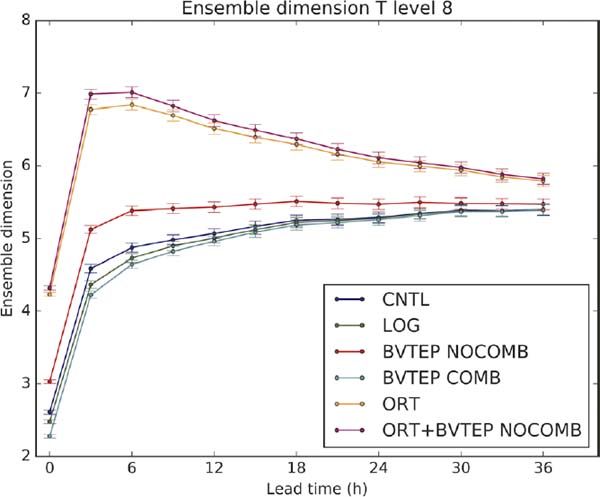
Ensemble dimension for temperature at model level 8 as a function of lead time for the different ensemble configurations tested.

Fig. 8.

Initial ensemble dimension for CNTL and BVTEP COMB over the test period.

4.3 Ensemble verification

The spread of an ensemble should represent the spread of the real underlying distribution. A Talagrand diagram or Rank Histogram can be constructed to test this property. Rank histograms for 850 hPa wind speed show underdispersive ensembles for all experiments (Fig. 9). However, experiments show different spreads, indicating the ability of each ensemble generation strategy to effectively introduce higher diversity in the forecast. BVTEP NOCOMB has a positive impact on the reduction of the number of outliers with respect to control, especially for short lead times when the influence of initial conditions is higher than the effects of boundary conditions, which are the same for all configurations. In this case, the introduction of multiple scales of interest into the initial perturbations through the exponential rescaling of the ABVs allows to sample a broader range of possible scenarios out-performing traditional ABVs. A considerable improvement is obtained using OBVs, and the combination of orthogonal bred vectors with the modification of the localization of perturbations provides the best results with a fairly flat histogram for a 6-h lead time and with a considerable improvement for longer lead times. Hence, the greater diversity obtained with OBV combined the positive impact of including multiple scales produces a more adequate sampling of the initial condition uncertainty. LOG and BVTEP COMB show similar rank histogram to CNTL, which is in agreement with the ensemble dimension results. Indeed, experiments with higher dimension (i.e., diversity) yield flatter rank histograms. Therefore, the rescaling used in the bred vector generation has no significant impact on mesoscale ensemble forecasts under realistic conditions, which is coherent with other studies (e.g., Corazza et al. 2003). Regarding precipitation, rank histograms also show an improvement in terms of lower frequencies of outliers for BVTEP NOCOMB, ORT, and ORT+BVTEP NOCOMB. However, for 3-h precipitation accumulations, differences among experiments are lower than for 850 hPa wind speed (Fig. 10).

Fig. 9.

Rank histogram for 850-hPa wind speed at lead times: a) 6 h, b) 12 h, c) 18 h and d) 24 h.

Fig. 10.

As in Fig. 9 for the 3-h accumulated precipitation.

An additional verification score, the CRPS, which is designed to measure the distance between the truth PDF and the forecasted one, is computed and analyzed for all experiments. In particular, CRPS for 850-hPa and 10-m wind speed (Figs. 11a, b) shows that the BVTEP NOCOMB and especially ORT and ORT+ BVTEP NOCOMB method improve upon the CNTL ensemble (i.e., lower CRPS), particularly for short lead times, being ORT+BVTEP NOCOMB the method which yields the best performance, whereas LOG and BVTEP COMB perform similarly to CNTL. The decomposition of CRPS into its different components reveals that the improvement in CRPS is related to an improvement in reliability, as resolution is very similar across experiments. Similar behavior is obtained for temperature (Figs. 11c, d), although the differences between experiments are lower. Given the large amount of available observations due to the use of analysis to perform the verification, confidence intervals are narrow, making small differences significant. Regarding 3-h precipitation accumulations against rain-gauge observations, ORT+BVTEP NOCOMB performs the best (Figs. 11e, f), especially for longer lead times, although the differences between experiments are not significant. The reason for this unexpected behavior is allegedly attributed to the spin-up time after a cold start of each 36-h forecast. The spin-up after a cold start is particularly important for precipitation fields. In addition, the bias score (Fig. 12) reveals a lower overprediction (Bias > 1) of 18- and 24-h forecasts for low thresholds, but a higher under-prediction (Bias < 1) for high thresholds. The greater number of low precipitation observations, which present a lower bias for longer lead times, could explain the behavior of CRPS, although the differences of CRPS with lead time are not significant. As for the wind speed and temperature, improvements in CRPS originate from better reliability.

Fig. 11.

CRPS and Reliability component of the CRPS as a function of lead time for the different experiments for a), b) 850-hPa (solid) and 10-m (dashed) wind speed; c), d) 850 hPa (solid) and 2 m (dashed) temperature; and e), f) 3-h accumulated precipitation. Error bars in panels e) and f) represent the 95 % confidence interval obtained from 1000 bootstrap samples. Error bars for wind and temperature are omitted because they are too narrow to be appreciated.

Fig. 12.

Bias score for 3-h accumulated precipitation as a function of precipitation thresholds for CNTL (blue) and ORT+BVTEP NOCOMB (magenta) at different lead times: 6 h (solid), 12 h (dashed), 18 h (dotted) and 24 h (dash-dotted). The plot includes reference Bias = 1 and the histogram of observation frequencies.

4.4 Case study

In order to better understand the impact of each perturbation generation strategy on ensemble skill, we focus our attention on a remarkable episode that occurred during the experimental test period. The different bred vectors produced in the cycles before the formation of the 7 November medicane illustrate characteristics of each method investigated. By design, it is expected that BVs highlight areas with strong instabilities, and thus, perturbations should focus on the medicane formation region. Indeed, ABVs and OBVs show perturbations concentrated near Sicily on 7 November at 00 UTC, whereas 12 h earlier, they are more scattered over the domain (Fig. 13). Despite the greater diversity of OBVs over the full domain, BVs of the cycle corresponding to 6 November at 12 UTC highlight regions in the vicinity of Sicily, whereas the maximums for ABVs are located near Corsica and Sardinia, as well as over the Adriatic. Therefore, in addition to producing larger spread, OBVs also emphasize better regions of high uncertainty than ABVs.

Fig. 13.

u-wind component of BVs at model level 5 (close to 925 hPa) for two ABVs (a, b and e, f) and two OBVs (c, d and g, h) bred vectors valid on 6 November 2014 at 12 UTC (a–d) and 7 November 2014 at 00 UTC (e–h). BV values represented are normalized to the 99.99 percentile.

Medicanes are a paradigmatic example of a high-impact phenomenon with low predictability. In order to assess the ability of CNTL and ORT+BVTEP NOCOMB to predict the event, the probability of sea level pressure below 990 hPa on 7 November at 12 UTC is computed for forecasts started 12h earlier. This time corresponds to the moment of maximum intensification of the medicane in analyses. The ORT+BVTEP NOCOMB experiment shows higher probabilities of low pressure and the region of low pressures is closer to the actual medicane than for the CNTL ensemble (Fig. 14).

Fig. 14.

Probability of sea level pressure below 990 hPa for a) CNTL and b) ORT+BVTEP NOCOMB ensembles (shaded) valid on 7 November 2014 at 12 UTC (T+12 h). Solid lines depict the sea level pressure analysis field.

In addition, the predicted medicane trajectories are inspected and compared with the observed cyclone track. The differences between CNTL and ORT+BVTEP NOCOMB are small (Fig. 15). Both ensembles have members close to the observed track during the first hours of simulation, passing through Malta. Nevertheless, none of the members is able to reproduce the final northward evolution of the medicane along the east coast of Sicily. The inclusion of model error in the ensembles and the use of a higher resolution in simulations could potentially improve the forecast for this extreme event. In addition, a domain centered over the region where the medicane formed would allow to emphasize the effect of initial condition perturbations from the effect of boundary conditions.

Fig. 15.

Medicane tracks for CNTL ensemble members (blue lines on the left panel) and ORT+BVTEP NOCOMB (magenta lines on the right panel) from 7 November at 12 UTC to 8 November at 06 UTC. Black line represents the observed track.

5. Conclusions

In this study, we explore the potential of bred vectors to contribute to the advancement of the prediction of mesoscale phenomena that produce high social impact. A fundamental challenge for mesoscale ensemble generation methods is the production of sufficient spread to adequately sample infrequent and extreme events in the distribution of predicted scenarios. We test the ability of arithmetic, logarithmic and orthogonal breeding techniques to generate improved mesoscale ensemble initial condition perturbations, and eventually better forecasts. Logarithmic bred vectors are rescaled using a geometrical mean norm instead of the original arithmetic norm. The use of orthogonalization processes improves upon the former, as collinearity among bred cycles is removed by design. Building upon this, we propose a method to generate ensemble initial condition perturbations containing a controllable range of spatial scales. These tailored perturbations allow the ensemble designer to target specific spatial scales of interest without modifying the bred rescaling period, typically forced by operational constraints.

By means of experimental ensembles run over a 3 month period with 2 forecasts per day and 36 h forecasts with 11 members, we benchmark each considered method with special attention on the ensemble diversity and skill. The ensemble diversity produced by each perturbation generation method is first tested with the so-called ensemble dimension, which quantifies the number of linearly independent members in the ensemble. In other words, this quantity measures the dimension of the subspace sampled by the perturbations. A first comparison between arithmetic and logarithmic experiments indicates that no significant differences are observed between them in terms of diversity. Despite the demonstrated differences between these two norms previously found in the literature for toy models, using LBVs does not have an impact with respect to the original ABVs in realistic mesoscale ensemble configurations. The fact that, conversely to toy models, realistic mesoscale ensembles run over limited area domains introduces the requirement for boundary conditions, and the system becomes non-autonomous. Thus, the need for boundary conditions in real models cancels the benefits of logarithmic rescaling reported for toy models. However, when orthogonalization is used, the diversity of the perturbations is significantly increased.

From the various flavors of BVs generated, multiple ensemble building strategies are tested. The original arithmetic method by Toth and Kalnay (1993) is labeled as control. The method of tailored perturbations clearly enhances ensemble diversity and skill when only the localization (spatial scale) of a BV is altered, but it is not the case when multiple BVs are combined into a single perturbation (i.e., in an ensemble member). Therefore, the results demonstrate that introducing (i.e., sampling) a wider range of scales in the initial condition perturbations than merely those dynamically generated by the breeding cycle improves ensemble diversity and skill. Contrary to the initial hypothesis, the linear combination of multiple modified perturbations damages the initial dimension and also ensemble forecast dimension at later lead times. The results confirm that the mesoscale generation method that produces the best diversity and verification results combines OBVs with tailored perturbations to generate initial perturbations that sample a wide range of spatial scales. Indeed, the key to its success is that the initially higher dimension of OBVs is enhanced with the tailored method, and the subsequent forecast also has considerably higher dimension than the other tested experiments for lead times up to 36 h. Additionally, this experiment exhibits the best forecast skill from the perspective of different verification scores. It is noteworthy that the results for ensemble dimension and the various verification scores are similar, so that the skill is improved when the ensemble dimension (i.e., the diversity) is higher.

Despite the significant improvements obtained from the new proposed method, all ensembles show some degree of underdispersion. This can partially be attributable to the particular configuration of the boundary conditions used (same boundary data for all experiments) and also to the presence of additional sources of error, such as model error, which is not sampled in these experiments.

The analysis of an extreme event occurred during the test period, the 7 November 2014 medicane, illustrates the characteristics of each ensemble initial condition generation method tested. ABVs and OBVs highlight the areas of intense instabilities prior to the formation of the medicane, as it is expected by the design of the breeding methodology. The performance of ensembles initiated from arithmetic, and orthogonal tailored bred vectors shows only minor differences among them in cyclone track, although the ORT+BVTEP NOCOMB experiment shows improvements in minimum pressure location for the time of maximum intensification

The potential of the new ensemble generation method consisting of the combination of OBVs with a tailored method to generate perturbations to initialize mesoscale ensemble prediction systems has been investigated and confirmed. These solid and promising results open the door to more ambitious tests, including the sampling of model error by means of multiphysics or stochastic parameterization setups, as well as larger ensemble sizes and higher spatial resolutions that allow the improvement the forecasts of severe weather phenomena in the short-range.

Acknowledgments

This work has been sponsored by FEDER/Ministerio de Ciencia, Innovación y Universidades - Agencia Estatal de Investigación/COASTEPS (CGL2017-82868-R). Author A. Hermoso received funding from the Spanish Ministerio de Educación, Cultura y Deporte (FPU16/05133). The authors thankfully acknowledge the computer resources granted at MareNostrum 4 and the technical support provided by Barcelona Supercomputing center (RES-AECT-2018-2-0010 and RES-AECT-2018-3-0009). We acknowledge the two anonymous reviewers and for their careful reading and their many insightful comments and suggestions, which improved the quality of the manuscript.

References

•  Anderson,  J., 1996: A method for producing and evaluating probabilistic forecasts from ensemble model integrations. J. Climate, 9, 1518-1530.
•  Annan,  J., 2004: On the orthogonality of bred vectors. Mon. Wea. Rev., 132, 843-849.
•  Berner,  J.,  G.  Shutts,  M.  Leutbecher, and  T.  Palmer, 2009: A spectral stochastic kinetic energy backscatter scheme and its impact on flow-dependent predictability in the ECMWF ensemble prediction system. J. Atmos. Sci., 66, 603-626.
•  Bowler,  N., 2006: Comparison of error breeding, singular vectors, random perturbations and ensemble Kalman filter perturbation strategies on a simple model. Tellus A, 58, 538-548.
•  Bretherton,  C. S.,  M.  Widmann,  V.  Dymnikov,  J.  Wallace, and  I.  Bladé, 1999: The effective number of spatial degrees of freedom of a time-varying field. J. Climate, 12, 1990-2009.
•  Buizza,  R.,  M.  Miller, and  T. N.  Palmer, 1999: Stochastic representation of model uncertainties in the ECMWF Ensemble Prediction System. Quart. J. Roy. Meteor. Soc., 125, 2887-2908.
•  Buizza,  R.,  P. L.  Houtekamer,  Z.  Toth,  G.  Pellerin,  M.  Wei, and  Y.  Zhu, 2005: A comparison of the ECMWF, MSC, and NCEP global ensemble prediction systems. Mon. Wea. Rev., 133, 1076-1097.
•  Buizza,  R.,  J.  Du,  Z.  Toth, and  D.  Hou, 2018: Major operational ensemble prediction systems (EPS) and the future of EPS. Handbook of Hydrometeorological Ensemble Forecasting.  Duan,  Q.,  F.  Pappenberger,  A.  Thielen,  J.  Wood,  H.  Cloke, and  J.  Schaake (eds.), Springer Berlin Heidelberg, 1-43.
•  Carrió,  D., and  V.  Homar, 2016: Potential of sequential EnKF for the short-range prediction of a maritime severe weather event. Atmos. Res., 178–179, 426-444.
•  Carrió,  D.,  V.  Homar,  A.  Jansa,  R.  Romero, and  M.  Picornell, 2017: Tropicalization process of the 7 November 2014 Mediterranean cyclone: Numerical sensitivity study. Atmos. Res., 197, 300-312.
•  Cavicchia,  L.,  H.  von Storch, and  S.  Gualdi, 2014: A longterm climatology of medicanes. Climate Dyn., 43, 1183-1195.
•  Clark,  A.,  J.  Kain,  D.  Stensrud,  M.  Xue,  F.  Kong,  M. C.  Coniglio,  K. W.  Thomas,  Y.  Wang,  J.  Brewster,  K.  Gao, and  X.  Wang, 2011: Probabilistic precipitation forecast skill as a function of ensemble size and spatial scale in a convection-allowing ensemble. Mon. Wea. Rev., 139, 1410-1418.
•  Corazza,  M.,  E.  Kalnay,  D. J.  Patil,  S.-C.  Yang,  R.  Morss,  M.  Cai,  I.  Szunyogh,  B. R.  Hunt, and  J. A.  Yorke, 2003: Use of the breeding technique to estimate the structure of the analysis “errors of the day”. Nonlinear Processes Geophys., 10, 233-243.
•  Du,  J.,  G.  DiMego,  B.  Zhou,  D.  Jovic,  B.  Ferrier, and  B.  Yang, 2015: Regional ensemble forecast systems at NCEP. Proceeding of 27th Conference on Weather Analysis and Forecasting/23rd Conference on Numerical Weather Prediction, Amer. Meteor. Soc., Chicago, 14 pp. [Available at https://ams.confex.com/ams/27WAF23NWP/webprogram/Paper273421.html.]
•  Dudhia,  J., 1989: Numerical study of convection observed during the winter monsoon experiment using a mesoscale two-dimensional model. J. Atmos. Sci., 46, 3077-3107.
•  Ehrendorfer,  M., 1994: The Liouville equation and its potential usefulness for the prediction of forecast skill. Part II: Applications. Mon. Wea. Rev., 122, 714-728.
•  Emanuel,  K., 2005: Genesis and maintenance of “Mediterranean hurricanes”. Adv. Geosci., 2, 217-220.
•  Fita,  L.,  R.  Romero,  A.  Luque,  K.  Emanuel, and  C.  Ramis, 2007: Analysis of the environments of seven Mediterranean tropical-like storms using an axisymmetric, nonhydrostatic, cloud resolving model. Nat. Hazards Earth Syst. Sci., 7, 41-56.
•  Gaume,  E.,  V.  Bain,  P.  Bernardara,  O.  Newinger,  M.  Barbuc,  A.  Bateman,  L.  Blaškovičová,  G.  Bloöschl,  M.  Borga,  A.  Dumitrescu, and  I.  Daliakopoulos, 2009: A compilation of data on European flash floods. J. Hydrol., 367, 70-78.
•  Gaume,  E.,  M.  Borga,  M.  Llasat,  S.  Maouche,  M.  Lang, and  M.  Diakakis, 2018: Mediterranean extreme floods and flash floods. The Mediterranean Region Under Climate Change. A Scientic Update, IRD Editions, 133-144.
•  Giggins,  B., and  G.  Gottwald, 2019: Stochastically perturbed bred vectors in multi-scale systems. Quart. J. Roy. Meteor. Soc., 145, 642-658.
•  Golub,  G., and  C.  VanLoan, 1996: Matrix Computations. Johns Hopkins University Press, 694 pp.
•  Greybush,  S.,  E.  Kalnay,  M.  Hoffman, and  R.  Wilson, 2013: Identifying Martian atmospheric instabilities and their physical origins using bred vectors. Quart. J. Roy. Meteor. Soc., 139, 639-653.
•  Haersbach,  H., 2000: Decomposition of the continuous ranked probability score for ensemble prediction systems. Wea. Forecasting, 15, 559-570.
•  Hasselmann,  K., 1976: Stochastic climate models. Part I. Theory. Tellus, 125, 2487-2515.
•  Hermoso,  A.,  V.  Homar, and  J.-I.  Yano, 2020: Exploring the limits of ensemble forecasting via solutions of the liouville equation for realistic geophysical models. Atmos. Res., 246, 105127, doi:10.1016/j.atmosres.2020.105127.
•  Hohenegger,  C., and  C.  Schär, 2007: Predictability and error growth dynamics in cloud-resolving models. J. Atmos. Sci., 64, 4467-4478.
•  Homar,  V.,  C.  Ramis, and  S.  Alonso, 2002: A deep cyclone of African origin over the Western Mediterranean: Diagnosis and numerical simulation. Ann. Geophys., 131, 93-106.
•  Hong,  S., and  J.  Lim, 2006: The WRF Single-Moment 6-Class Microphysics Scheme (WSM6). J. Korean Meteor. Soc., 42, 129-151.
•  Janjic,  Z., 1994: The step-mountain eta coordinate model: Further developments of the convection, viscous sublayer, and turbulence closure schemes. Mon. Wea. Rev., 122, 927-945.
•  Kain,  J., 2004: The Kain-Fritsch convective parameterization: An update. J. Appl. Meteor., 43, 170-181.
•  Kalnay,  E., 2003: Atmospheric Modeling, Data Assimilation and Predictability. Cambridge University Press, 341 pp.
•  Kalnay,  E., 2008: Bred vectors: Theory and applications in operational forecasting. Lecture 3, Alghero, Italy, 33 pp. [Available at https://www2.atmos.umd.edu/∼ekalnay/syllabi/AOSC614/Alghero-Kalnay3-BVsApplications.ppt.pdf.]
•  Kalnay,  E.,  M.  Corazza, and  M.  Cai, 2002: Are bred vectors the same as Lyapunov vectors? Proceeding of EGS XXVII General Assembly, Nice, EGU. [Available at https://ams.confex.com/ams/annual2002/techprogram/paper_28833.htm.]
•  Keller,  J.,  A.  Hense,  L.  Kornblueh, and  A.  Rhodin, 2010: On the orthogonalization of bred vectors. Wea. Forecasting, 25, 1219-1234.
•  Llasat,  M. C.,  M.  Llasat-Botija,  O.  Petrucci,  A. A.  Pasqua,  J.  Rosselló,  F.  Vinet, and  L.  Boissier, 2013: Towards a database on societal impact of Mediterranean floods within the framework of the HYMEX project. Nat. Hazards Earth Syst. Sci., 13, 337-1350.
•  Lorenz,  E. N., 1963: Deterministic nonperiodic flow. J. Atmos. Sci., 20, 130-141.
•  Matheson,  J., and  R.  Winkler, 1976: Scoring rules for continuous probability distributions. Manage Sci., 22, 1051-1173.
•  Michaelides,  S.,  J.  Karacostas,  J. L.  Sánchez,  A.  Retalis,  I.  Pytharoulis,  V.  Homar,  R.  Romero,  P.  Zanis,  C.  Giannakopoulos,  J.  Bühl, and  A.  Ansmann, 2018: Reviews and perspectives of high impact atmospheric processes in the Mediterranean. Atmos. Res., 208, 4-44.
•  Mlawer,  E. J.,  S. J.  Taubman,  P. D.  Brown,  M. J.  Iacono, and  S. A.  Clough, 1997: Radiative transfer for inhomogeneous atmospheres: RRTM, a validated correlated-k model for the longwave. J. Geophys. Res., 102, 16663-16682.
•  Molteni,  F.,  R.  Buizza,  T. N.  Palmer, and  T.  Petroliagis, 1996: The ECMWF ensemble prediction system: Methodology and validation. Quart. J. Roy. Meteor. Soc., 122, 73-119.
•  Nadarajah,  S., 2005: A generalized normal distribution. J. Appl. Stat., 32, 685-694.
•  Nutter,  P.,  D.  Stensrud, and  M.  Xue, 2004: Eects of coarsely resolved and temporally interpolated lateral boundary conditions on the dispersion of limited-area ensemble forecasts. Mon. Wea. Rev., 132, 2358-2377.
•  Palmer,  T., 2018: The ECMWF ensemble prediction system: Looking back (more than) 25 years and projecting forward 25 years. Quart. J. Roy. Meteor. Soc., 145, 12-24.
•  Patil,  D.,  B.  Hunt,  E.  Kalnay,  J.  Yorke, and  E.  Ott, 2001: Local low dimensionality of atmospheric dynamics. Phys. Rev. Lett., 86, 5878-5881.
•  Pazó,  D.,  M.  Rodríguez, and  J.  López, 2011: Maximizing the statistical diversity of an ensemble of bred vectors by using the geometric norm. J. Atmos. Sci., 68, 1507-1512.
•  Primo,  C.,  M. A.  Rodríguez,  J. M.  López, and  I.  Szendro, 2005: Predictability, bred vectors, and generation of ensembles in space-time chaotic systems. Phys. Rev. E: Stat., Nonlinear, Soft Matter Phys., 72, 015201, doi:10.1103/PhysRevE.72.015201.
•  Primo,  C.,  M.  Rodríguez, and  J.  Gutiérrez, 2008: Logarithmic bred vectors. A new ensemble method with adjustable spread and calibration time. J. Geophys. Res., 113, D05116, doi:10.1029/2007JD008998.
•  Romero,  R.,  C.  Ramis,  S.  Alonso,  C.  Doswell, and  D.  Stensrud, 1998: Mesoscale model simulations of three heavy precipitation events in the western Mediterranean region. Mon. Wea. Rev., 126, 1859-1881.
•  Saito,  K.,  H.  Seko,  M.  Kunii, and  T.  Miyoshi, 2012: Effect of lateral boundary perturbations on the breeding method and the local ensemble transform Kalman filter for mesoscale ensemble prediction. Tellus A, 64, 11594, doi:10.3402/tellusa.v64i0.11594.
•  Saslo,  S., and  S.  Greybush, 2017: Prediction of lake-effect snow using convection-allowing ensemble forecasts and regional data assimilation. Wea. Forecasting, 32, 1727-1744.
•  Skamarock,  W.,  J.  Klemp,  D. O.  Dudhia,  J.  Gill,  D.  Barker,  M. G.  Duda,  X.-Y.  Huang,  W.  Wang, and  J. G.  Powers, 2008: G.: A description of the Advanced Research WRF version 3. NCAR Tech. Note NCAR/TN-475+STR.
•  Stensrud,  D.,  J.  Bao, and  W.  T., 2000: Using initial condition and model physics perturbations in short-range ensemble simulations of mesoscale convective systems. Mon. Wea. Rev., 128, 2077-2107.
•  Talagrand,  O.,  R.  Vautard, and  B.  Strauss, 1997: Evaluation of probabilistic prediction systems. Proceeding of ECMWF Workshop on Predictability, Reading, United Kingdom, ECMWF, 25 pp.
•  Tewari,  M.,  F.  Chen,  W.  Wang,  M.  Dudhia,  J.  LeMone,  K.  Mitchell,  M.  Ek,  G.  Gayno,  J.  Wegiel, and  R. H.  Cuenca, 2004: Implementation and verification of the unified Noah land surface model in the WRF model. Proceeding of 20th Conf. on Weather Analysis and Forecasting/16th Conf. on Numerical Weather Prediction, Seattle, WA, Amer. Meteor. Soc. [Available at https://ams.confex.com/ams/84Annual/techprogram/paper_69061.htm.]
•  Toth,  Z., and  E.  Kalnay, 1993: Ensemble forecasting at NMC: The generation of perturbations. Bull. Amer. Meteor. Soc., 74, 2317-2330.
•  Toth,  Z., and  E.  Kalnay, 1997: Ensemble forecasting at NCEP and the breeding method. Mon. Wea. Rev., 125, 3297-3319.
•  Tudurí,  E., and  C.  Ramis, 1997: The environments of significant convective events in the Western Mediterranean. Wea. Forecasting, 12, 294-306.
•  Warner,  T.,  R.  Peterson, and  R.  Treadon, 1997: A tutorial on lateral boundary conditions as a basic and potentially serious limitation to regional numerical weather prediction. Bull. Amer. Meteor. Soc., 78, 2599-2618.
•  Wei,  M.,  Z.  Toth,  R.  Wobus, and  Y.  Zhu, 2008: Initial perturbations based on the ensemble transform (ET) technique in the NCEP global operational forecast system. Tellus A, 60, 62-79.
•  Yamaguchi,  M.,  T.  Iriguchi,  T.  Nakazawa, and  C.  Wu, 2009a: An observing system experiment for Typhoon Conson (2004) using a singular vector method and DOTSTAR data. Mon. Wea. Rev., 137, 2801-2816.
•  Yamaguchi,  M.,  R.  Sakai,  M.  Kyoda,  T.  Komori, and  T.  Kadowaki, 2009b: Typhoon ensemble prediction system developed at the Japan meteorological agency. Mon. Wea. Rev., 137, 2592-2604.
•  Zhu,  J.,  F.  Kong, and  H.  Lei, 2012: A regional ensemble forecast system for stratiform precipitation events in northern China. Part I: A case study. Adv. Atmos. Sci., 29, 201-216.
•  Zhu,  J.,  F.  Kong, and  H.  Lei, 2013: A regional ensemble forecast system for stratiform precipitation events in northern China region. Part II: Seasonal evaluation for summer 2010. Adv. Atmos. Sci., 30, 15-28.