Abstract
Ultra-high-resolution numerical weather prediction (NWP) experiments over a large domain have been conducted to investigate the impacts of different factors of an NWP model in simulating the Hiroshima heavy rain event in August 2014. This is a continuation of the study in Part 1 in which similar experiments were carried out for the Izu Oshima heavy rain event in October 2013. We have demonstrated the benefit of using a high-resolution model (500-m grid spacing or less) with a large domain in simulating torrential rain events.
The simulated location and intensity of the rain band in the Hiroshima case has been shown to be sensitive to the model resolution. The simulation at the 2-km grid spacing could reproduce the rain band, but with a shift to the northeast. This displacement error was reduced when the grid spacing was further reduced to 500 m and 250 m. The best simulation both in the location and intensity was obtained at the 250-m grid spacing. The planetary boundary layer schemes had a smaller impact in this case, which is different from the Izu Oshima case.
This study also investigated the dependency of simulated convective cores (CCs) on model resolutions. The local rate of change of the number of CCs with respect to the model resolution was found to start decreasing at very high resolutions that are around the 500-m grid spacing. This implies the number of CCs tends to converge when the resolution goes beyond 500 m.
1. Introduction
In recent years, disasters related to heavy rainfalls have become more frequent in Japan. Typical examples are the heavy rainfall events that caused debris flows in Izu Oshima on October 15–16, 2013 and Hiroshima City on August 19–20, 2014. An investigation by the Japan Meteorological Agency (JMA) into the trend of heavy rainfall events with hourly precipitation greater than 80 mm from 1976 to 2015 found a near-certain increase in the number of these events (Japan Meteorological Agency 2016). Ogura (1991) found that most heavy rainfalls in Japan were associated with the back-building pattern in which new convective cells are generated in the flow upstream and form a line-shaped rain band. This back-building mechanism has also been observed in recent heavy rainfall events (Meteorological Research Institute 2011, 2012, 2014, 2016, 2017).
To mitigate the potential damage caused by heavy rainfall, a reliable numerical weather prediction (NWP) system is vital. The forecast performance of an NWP system is determined by the initial and boundary conditions digested into its numerical model and, of course, the model itself. Initial conditions can be improved by using more sophisticated data assimilation methods and introducing more observations into the assimilation process (Kalnay 2003; Lahoz et al. 2010). In this study, we focus only on the impact of different aspects of an NWP model on its forecast quality assuming ideal initial and boundary conditions, therefore we employed analyses as initial and boundary conditions.
The forecast quality of an NWP model is affected by many factors including its dynamic core, the physical processes parameterized inside, the integration domain, and the resolution. For example, fine grid spacings can resolve deep moist convection, reduce discretization errors, and make terrain more realistic (Bryan et al. 2003; Roberts and Lean 2008; Roberts et al. 2009; Oku et al. 2010; Bryan and Morrison 2012; Nunalee et al. 2015; Takemi 2018). Another example is the choice of the planetary boundary layer (PBL) schemes when the model is run at the “gray zone” where turbulence length scales are comparable to horizontal resolutions (Wyngaard 2004).
In Part 1 (Oizumi et al. 2018), we examined the impact of some of these factors in forecasting the Izu Oshima heavy rain event with a regional NWP model named the JMA nonhydrostatic model (JMA-NHM, hereafter simply mentioned as “NHM”; Saito et al. 2006, 2007; Saito 2012) running in the Japanese supercomputer “K” (Miyazaki et al. 2012). We have shown that the location of the rain band in this case was very sensitive to the PBL schemes and the domain sizes. Also, as expected, fine grid spacings combined with fine terrain data improved the prediction of intense rain considerably.
This part (Part 2) continues the work in Part 1 for another heavy rainfall event that occurred in Hiroshima on August 19–20, 2014 to see whether the findings in Part 1 hold for another case whose spatial scales and mechanism that caused the heavy rain are very different from those considered in Part 1. Kita et al. (2016) simulated this event using the Weather Research and Forecasting model with a 1-km grid spacing. Although the rainfall distribution was reproduced, the intense rain area was shifted to the northeast compared to the observation. It is interesting to know whether we will see the same displacement with the NHM and determine which factors lead to such displacement. Moreover, we examine in detail the dependency of deep moist convection on grid spacing owing to the crucial role of deep convection in simulating heavy rain. This work was not done in Part 1 for the Izu Oshima case.
This paper is organized as follows. A detailed description of the Hiroshima heavy rain event is given in Section 2. Experimental settings to simulate this event with the NHM are described in Section 3. The resulting simulations are presented in Section 4, where impacts of model resolutions and PBL schemes are examined. Section 5 is devoted to sensitivity tests on model domain sizes and terrain data. Section 6 investigates the dependency of convective simulations on model resolutions in detail. Finally, Section 7 summarizes the results obtained in the study.
2. Hiroshima heavy rainfall event on August 19–20, 2014
Between July 30 and August 26, 2014, heavy rainfall occurred in many locations in Japan (Japan Meteorological Agency 2014a). Figure 1 shows the synoptic weather chart at 03 JST (Japan Standard Time, +9 UTC) on August 20, 2014, where a stationary front from the south of China to the west of Hokkaido can be identified. The main island of Japan and Kyushu were in the warm sector of the front.

Figure 2a shows the accumulated precipitation in this peak period over western Japan estimated by the JMA's precipitation analysis system, where several intense rain bands from southwestern to northwestern Kyushu can be observed. In particular, near Hiroshima city, an intense line-shaped rain band occurred with an approximate length and width of 100 km and 20–30 km, respectively (see Fig. 2b). This rain band was formed when the warm moist air flowed through the Bungo channel into the southeastern part of Yamaguchi and induced the development of back-building convective systems around the border of Yamaguchi and Hiroshima (Japan Meteorological Agency 2014b). The maximum precipitation of 246 mm was registered over this period.

A terrain map of the Hiroshima prefecture derived from a digital map with a 10-m grid spacing is shown in Fig. 3. According to the map, Hiroshima city is in a narrow plain surrounded by mountains, with its south side facing the bay of Hiroshima. The back-building convective systems occurred at the mountainous areas that are marked by the white circle in Fig. 3a (Japan Meteorological Agency 2014b). The debris flows occurred on the southeastern slope of the mountainous areas, which are marked by the hatched circles in Fig. 3b. Figure 4 shows the 10-minute precipitations and the accumulated precipitations at the two rain gauges Miiri and Kasugano, which are marked by the two black points in Fig. 3b. At both the sites, intense rain started around 01 JST on August 20, and the accumulated precipitation exceeded 200 mm after 3 hours.
3. Experimental settings
As in Part 1, the optimized version of the NHM for the K computer (Oizumi et al. 2015) was used in this study. The NHM was run over a domain that covered the Japanese mainland (the largest domain in Fig. 5), which was identical to the former domain used by the JMA's Local Forecast Model (Japan Meteorological Agency 2013). Figure 5 also shows several smaller domains that are described when we encounter them later. As described in the Introduction, as we do not examine the impact of initial and boundary conditions, those fields in all experiments were interpolated from the JMA's mesoscale analyses (MA) (Japan Meteorological Agency 2013). The update frequency for the boundary conditions was set to 3 hours. All the simulations were started at 21 JST on August 19 and run until 06 JST on August 20.

To examine the impact of resolutions on the simulations, the NHM was run at four different grid spacings of 5 km, 2 km, 500 m, and 250 m. The number of horizontal grid points and the number of vertical levels varied depending on the grid spacing used in each experiment. The terrains at those resolutions were derived from the Global 30 arc-second elevation dataset (GTOPO30) (https://lta.cr.usgs.gov/GTOPO30), which originally has a grid spacing of approximately 1 km. The topographical slopes between adjacent grid points were limited to 15 % in the preprocessing.
Similarly, to examine the impact of the PBL schemes, two PBL schemes were considered, that is, the Mellor–Yamada–Nakanishi–Niino level 3 scheme (MY) (Nakanishi and Niino 2004, 2006) and the Deardorff scheme (DD) (Deardorff 1980). Owing to the nature of these schemes, we applied only the MY scheme at the 5-km grid spacing and the DD scheme at the 250-m grid spacing. However, for intermediate grid spacings between 2 km and 500 m, we applied both the schemes to infer which PBL scheme is more appropriate at such a grid spacing. At the 5-km grid spacing, the impact of cumulus parameterization (CM) was investigated by running two simulations: one with the modified Kain–Fritsch (KF) scheme and another without the CM. However, for all the experiments with grid spacings finer than 5 km, we did not employ CM. All other parameterization schemes were set the same among all the experiments.
In summary, each experiment was determined by three factors: the CM scheme, the grid spacing, and the PBL scheme. Therefore, each experiment was assigned a name formed by concatenating the short name of the CM scheme (KF or CM), the grid spacing (5 km, 2 km, 500 m, or 250 m), and the short name of the PBL scheme (MY or DD). These experiments are listed and explained in Table 1.
4. Results
4.1 Verification
Figure 6 shows the 3-hour accumulated precipitations simulated by the six experiments KF5kmMY, CM2kmMY, CM2kmDD, CM500mMY, CM500mDD, and CM250mDD valid at the same time as the observation in Fig. 2a. It is more appropriate to use CM5kmMY for a fair comparison. However, without CM, the simulation at the 5-km grid spacing could not produce intense rain and as a result, was worse than KF5kmMY (not shown here). Clearly, there is a distinct difference between KF5kmMY and the others, where KF5kmMY underestimated all precipitation areas except the rain band in the northwest of Kyushu. It is interesting to see that the remaining experiments somehow yielded the same precipitation distributions, despite the differences in the resolutions and the PBL schemes.

To see the significant differences in the simulations, we focus on the 3-hour accumulated precipitations around Hiroshima city as depicted in Fig. 7, of which the corresponding observation is given in Fig. 2b. A distinct line-shaped rain band can be identified easily in all the experiments except KF5kmMY. It becomes clear that the experiments with the 2-km grid spacing had displacement errors in simulating this rain band in which its location was shifted to the northeast compared with the observation. These biases were reduced when decreasing the grid spacing to 500 m and 250 m. At the 500-m grid spacing, CM500mDD simulated the intense rain area better than CM500mMY, showing the more important role of the DD scheme at such a resolution.

To further assess those models' performance, the precipitation intensity, distribution, and time lag were evaluated by using the Fractions Skill Score (FSS) (Robert and Lean 2008; Duc et al. 2013). The verification was performed for the 1-hour precipitations from 23 JST August 19 to 05 JST on August 20 over domain C shown in Fig. 5. The FSS intensity-scale diagrams for KF5kmMY, CM2kmMY, CM500mDD, and CM250mDD are presented in Figs. 8a–d, respectively, while the FSS differences among them are presented in Figs. 8e–g.

For KF5kmMY (Fig. 8a), the FSSs for the thresholds ≥ 10 mm h−1 are 0.0, indicating that KF5kmMY was capable only of reproducing light and moderate rain. In contrast, for CM2kmMY (Fig. 8b), the FSSs for the same thresholds are between 0.05 and 0.24. This difference shows that CM2kmMY yielded better simulations than KF5kmMY at intense rainfall thresholds. Moreover, this tendency holds for other rainfall thresholds as well. If we continue to increase the resolution, CM500mDD (Fig. 8c) further improved rainfall forecast, especially for intense rain (Fig. 8f). At the highest resolution, CM250mDD (Fig. 8d) outperformed CM500mDD for thresholds ≥ 40 mm h−1 (Fig. 8g).
4.2 Simulated back-building convective systems
As the verification pointed out that the other experiments were significantly more skillful than KF5kmMY, we examined the performances of CM2kmMY and CM500mDD in simulating the back-building convective systems. The reason for choosing these two experiments is the fact that they were the best simulations at their grid spacings. Figure 9a shows the vertical velocities w at the height z = 1 km simulated by CM500mDD at three consecutive times 01h10′, 01h20′, and 01h30′ JST on August 20. Here, the lines AB indicate the main lines along which the intense rain occurred (Fig. 7e). Along these lines, the updrafts were 2–4 m s−1 at the prefectural border where convective clouds started to develop and increased to 3–6 m s−1 at Hiroshima city (the arrows in Fig. 9a).
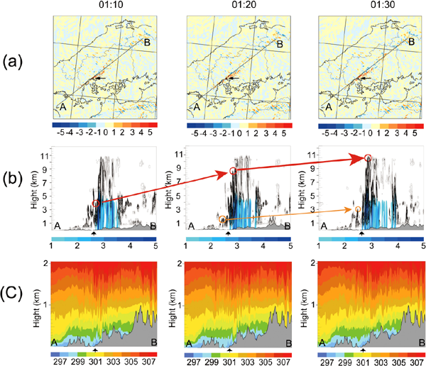
Figure 9b shows the vertical cross-sections of the cloud and rain mixing ratios (qc and qr) through the lines AB. It can be seen that cumulonimbus clouds developed around Hiroshima city and could reach as high as 11 km. As a result, the large qr areas in the leeside of these cumulonimbus clouds brought intense rain as well as graupel and snow (not shown here). The evolutions of some typical convective cells are marked by the red and orange arrows. These evolutions illustrate clearly the work of back-building convective systems in which convective cells are formed continuously in the flow upstream and maintained an intense rain band in the flow downstream. Figure 9c shows the vertical cross-sections of the potential temperatures θ along the lines AB. The cold air with θ lower than 298 K existed near the surface of the windward side of Hiroshima city where the cumulonimbus clouds developed.
Similarly, CM2kmMY could also reproduce the back-building convective systems as seen in Fig. 10, but with a shift of the rain band to the northeast. Here, we used the lines CD to indicate the lines along which the intense rain concentrated, which are, of course, not identical to the lines AB in Fig. 9. Note that the times in Fig. 10a (02h25′, 02h35′, and 02h45′ JST) are not the same as those in Fig. 9a. As CM2kmMY had a resolution coarser than CM500mDD, the number of simulated convective cells as identified in Fig. 10b is much less than those in Fig. 9b. In Fig. 10c, The cold air with θ lower than 299 K existed near the surface of Hiroshima city where the cumulonimbus clouds developed. The cloud tops simulated by CM2kmMY were also lower than those simulated by CM500mDD. These differences are the easiest to be observed in the three-dimensional visualizations of the back-building convective systems simulated by CM500mDD and CM2kmMY in Fig. 11. Compared with the JMA's high-resolution precipitation nowcast (JMA 2014b), the sizes of the convective cells in CM2kmMY are much larger, which are less realistic.

The verification shows that the simulation was improved when we increased the resolution and switched the PBL scheme to the DD scheme. To know which factor is more important in this case, we compared the averaged vertical profiles of different variables over area A in Fig. 5 and the interval 00-01 JST on August 20 as simulated by CM500mMY and CM500mDD in Fig. 12. In general, the averaged vertical profiles of CM500mMY for θ, specific humidities qv, equivalent potential temperatures θe, and horizontal wind speeds uv were slightly higher than those of CM500mDD, implying that CM500mMY yielded larger vertical mixing in the boundary layer. This tendency is consistent with the result in Part 1, but the differences in this case are much smaller than those in the Izu Oshima case.

This result implies that to improve the simulation, the resolution plays a crucial role in the Hiroshima case. This is different from the Izu Oshima case in Part 1. One of the reasons for this may be attributed to the differences in the formation of the rain bands. In the Izu Oshima case, the rain band was formed along a stationary front over the sea when a strong typhoon was approaching. Consequently, the PBL schemes strongly influenced the up/down-draft pairs in the windward/lee sides of the front and the formation of cold pools. In contrast, in the Hiroshima case, the rain band was developed in a humid warm air region approximately 300 km away from the south of the synoptic-scale front. The difference between the sizes of the rain bands in the two cases may also play an important role here. In fact, the length and width of the rain band in the Izu Oshima case were approximately three times larger than those of the Hiroshima case. Therefore, to simulate the formation of the rain band accurately, a higher resolution is needed.
5. Sensitivity tests
5.1 Impact of domain sizes
All conclusions in Section 4 so far are drawn from the NHM runs with a very large domain. To check whether the conclusions would still hold if the NHM used a smaller domain, the two experiments CM2km
MY and CM500mDD were rerun with the small domain in Fig. 5, which covered a 200-km2 region around Hiroshima city. These experiments could use either the MA or the simulations provided by the NHM runs with the large domain as their initial and boundary conditions. If the latter was adopted, the nested simulations were started at 22 JST on August 19 with 8-hour simulations to mitigate the impact of spin-up problems from the nesting simulations. To differentiate those experiments from the original ones, suffixes were added to the names CM2kmMY and CM500mDD, which indicate the ways in which the initial and boundary conditions were digested into the simulations. These suffixes are listed and explained in Table 2.

Similar to Fig. 7, Fig. 13 shows the 3-hour accumulated precipitations from those additional experiments. At the 2-km grid spacing, all the experiments with the small domain shifted the location of the rain band to the northeast compared to CM2kmMY. The maximum rain intensity was also weaker than that of CM2km-MY. However, at the 500-m grid spacing, these experiments reproduced the rain band at a location similar to CM500mDD, although the simulated intensity was still weaker than that of CM500mDD. When we increased the resolution from 2 km to 500 m, the rain intensity became significantly weaker, especially if the nesting procedure was applied (Figs. 13b–d compared with Figs. 13f–h). One of the reasons was that the outer model of the former, that is, KF5kmMY, was not capable of reproducing the intense rain band (Fig. 7a). Again, we see that the rain band was simulated more accurately in both location and intensity when we refined the grid spacing from 2 km to 500 m. This highlights the important role of the horizontal resolution over the model domain size in this case.

In Part 1, when the grid spacing was the same, the precipitation distribution was improved with a more realistic topography. In the present case, the convective clouds associated with the rain band were generated in the mountainous area. Thus, it is interesting to check again whether finer terrain data can improve the simulated precipitation distribution or not.
First, with the same settings as CM500mDD, we examined the role of the terrain in the formation of the rain band by removing the terrain in area B (in Fig. 5) around Hiroshima city (Fig. 14a). Figure 14b shows the 3-hour accumulated precipitations given by this experiment, which we named CM500mDD_no_topo. Compared with the original simulation in Fig. 7e, the location of the rain band was shifted leeward (to the northeast) and the maximum rainfall intensity was lower. This was probably caused by the late formation of convective clouds triggered by the terrain in the Yamaguchi prefecture. Therefore, the terrain around Hiroshima city seemed to contribute to the rapid development of the observed convective clouds.

Second, instead of the dataset GTOPO30, we derive the terrain data at grid spacings of 500 m and 250 m from the digital elevation data with the 50-m grid spacing provided by the Geospatial Information Authority of Japan (KTOPO). Then, we rerun the two experiments CM500mDD and CM250mDD with the new terrain data and named them CM500mDD_K and CM250mDD_K, respectively. The 3-hour accumulated precipitations that resulted from these additional experiments are shown in Figs. 14c and 14d. In both the cases, the locations of the rain band were similar to those simulated by the original experiments, although the maximum rain intensities were slightly different. Therefore, to quantify the impact of the terrain data on the precipitations, we used the FSS and the verification result is shown in Fig. 14e. The FSS reveals that the KTOPO slightly improved the rainfall simulations in this case.
6. Dependency of simulated convective cores on model resolutions
6.1 Analysis method
The methodology used to detect and analyze the simulated convection was adapted from Miyamoto et al. (2013) with some modifications and is illustrated in Fig. 15. In step 1, the liquid water path (LWP) field was estimated by integrating the liquid water content vertically from 2 km to 6 km. The resulting LWP field is shown in step 2, where the colored boxes represent convective grids (CGs). Here, a model grid point was considered as a CG if its LWP was greater than 0.1 kg m−2. Based on the CGs, convective cores (CCs) were defined as all local maxima of the averaged vertical velocities w̄ over the CGs with the maximum values greater than a threshold. The same definition was used in Algorithm 1 in Sueki et al. (2019). For consistency with the use of the LWP, w̄ was averaged from 2 km to 6 km and the threshold of 0.5 m s−1 was selected. The local maxima of w̄ are highlighted in red over the CG points in step 3. Note that all the neighboring grids of a CC must be CGs to be considered as valid CCs.

After the CCs were detected, their statistical features could be derived from the vertical velocities w around these cores. Thus, step 4 depicts a three-dimensional w field surrounding the CCs detected in step 3. Note that w need not be confined to the heights between 2 km and 6 km. The composite field of w was calculated by averaging w around all individual CCs. At each vertical level, the contours of the composite field tended to form concentric circles. This suggested that the composite field can be described more compactly by averaging the composited w along each circle. This calculation is illustrated in step 5. Finally, the resulting radius–height composite map of w is obtained in step 6, where the vertical axis indicates the height z and the horizontal axis indicates the radius r, which is a multiple of grid points. All features of the simulated convection were drawn from such kinds of composite maps.
To illustrate the work of the algorithm, we show in Figs. 16a–c the simulated w fields at z = 4.2 km, and the detected CGs and CCs from CM2kmMY, CM500mDD, and CM250mDD at 0200 JST on August 20. The result given by KF5kmMY is not shown as no CCs were detected at this time.
6.2 Characteristics of convective cores
Figure 17 shows the dependency of the number of CCs on the resolution in the logarithm scales for the two groups of simulations: those using the MY scheme and those using the DD scheme. Here, the number of CCs was taken as the average over the period from 22 JST on August 19 to 06 JST on August 20, with a time step of 1 hour. As expected, the number of CCs increases with the increasing model resolution. It is also interesting to see that the numbers of CCs are not very different between the two PBL schemes. In the case of the MY scheme, we also plotted the number of CCs simulated by CM5kmMY to check the impact of convective parameterization. It is clear that convective parameterization decreased the number of CCs considerably.

Figure 17 enables us to answer the question: what is the increasing rate of the number of CCs with respect to the model resolution? Using the logarithm scale, this local rate of change at each resolution Δx is given by α = −dlog(N )/dlog(Δx), where N is the number of CCs. When increasing the resolution from 5 km (KF5kmMY) to 2 km (CM2kmMY), the number of CCs increases about 8.3 times, implying the approximated α = 2.3. However, if we consider CM5kmMY instead of KF5kmMY, the number of CCs increases by only 5.5 times and α drops to 1.9. This increasing rate in the number of CCs is about 15 times if we go further from the resolution of 2 km to 500 m, leading to the same value of α = 1.9. Finally, if Δx changes from 500 m to 250 m, α now reduces to 1.2. This means that α is around 2.0 for resolutions coarser than 500 m and becomes smaller for finer resolutions. This result is somewhat different from Miyamoto et al. (2013), in which α is about 2.0 with grid spacings greater than 3.5 km and decreases slightly with the decrease in grid spacings from 3.5 km to 1.7 m.
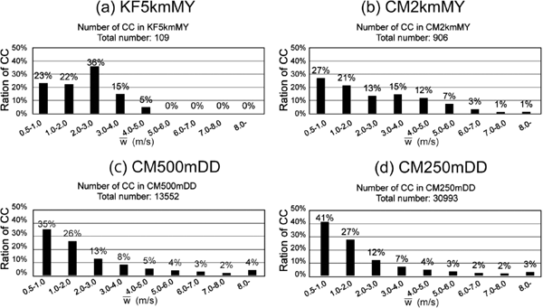
Figure 18 shows the histograms of the numbers of CCs classified against the intensities of updraft represented by w̄ for the four experiments KF5kmMY, CM2kmMY, CM500mDD, and CM250mDD. In KF5kmMY (Fig. 18a), the relative ratio of the number of CCs at the bin 2.0–3.0 m s−1 is the largest (about 36 %); no CCs appear when w̄ > 5.0 m s−1. However, this largest ratio is 27 % at the bin 0.5–1.0 m s−1 for CM2kmMY (Fig. 18b) and the CCs were detected even at w̄ > 5.0 m s−1. Like CM2kmMY, the numbers of CCs in CM500mDD (Fig. 18c) and CM250mDD (Fig. 18d) tend to decrease as w̄ increases, with the peak on the left-most bin 0.5–1.0 m s−1.
The radius–height composite maps of w for the CCs simulated by the four experiments are shown in Fig. 19a. In all cases, the w fields around the CCs have spindle shapes, which attain the maximum around the heights z = 4.2–4.5 km. The top heights of w > 0.5 m s−1 decrease from 8.4 km to 7.2 km with the increasing resolution. The spindle shape tends to expand horizontally in the upper part when the resolution becomes higher. This is probably because convective updrafts as expressed in the composited map of w are more influenced by horizontal winds and the tilting of convective cells at very high resolutions.
Figure 19b shows the magnitude of w against the distance from the center of a CC at the height where w attain its maximum. In the experiments without CM, the maximum w decreases with the increasing resolution. This can be attributed to the fact that many weak CCs are detected when the resolution is increased. In CM500mDD and CM250mDD, the magnitudes of w away from the center of the CC were nearly flat around 0.4–0.5 m s−1. As seen in Figs. 16b and 16c, many CCs were detected at these resolutions and the average values of w away from the CC center were contaminated by other nearby convection cells. Further investigations into the characteristics of CCs are necessary in the future, with a more sophisticated method to define CCs.
7. Summary and conclusion
In this study, ultra-high-resolution NWP experiments over a large domain were conducted to investigate the impacts of some different factors of the NWP model NHM in simulating the Hiroshima heavy rain event in August 2014. This is a continuation of the study in Part 1 in which similar experiments were carried out for the Izu Oshima heavy rain event in October 2013. The two events are different, both in the mechanisms that caused the heavy precipitations and in the spatial scales of the rain bands. It is important to know what factors should be considered in each event as this can contribute significantly to improve forecasts in the future. In addition, this part also investigates the dependency of simulated convective cells on model resolutions, a topic that was not addressed in Part 1.
The resolution has been shown to play a crucial role if we want an accurate simulation in the Hiroshima case. The simulation at the 5-km grid spacing could not reproduce the rain band, whereas that at the 2-km grid spacing could reproduce the rain band, but with a shift to the northeast. This displacement error was reduced when the grid spacing was further reduced to 500 m. At the 250-m grid spacing, the model simulated the rain band well in both the location and the intensity. The PBL schemes had a smaller impact in this case than in the Izu Oshima case, which can be explained by two facts: (1) the rain band was far from the synoptic front; and (2) the rain band had quite a small size of approximately 100 km.
Sensitivity tests on model domain sizes have pointed out that all conclusions still hold if the model domain becomes smaller. Of course, if the nesting procedure was employed, the nesting models should also have fine enough resolutions. Other sensitivity tests on terrain data showed that the rapid development of the observed convective cells was probably triggered by the terrain at the windward side around Hiroshima city. Also, as in Part 1, the terrain data derived from the KTOPO could slightly improve precipitation simulations if compared with those derived from the GTOPO.
The dependency of the simulated CCs on model resolutions was investigated by modifying the method introduced by Miyamoto et al. (2013). The local rate of change of the number of CCs with respect to the model resolution was found to start decreasing at very high resolutions of around 500-m grid spacing. This implies that the number of CCs tends to converge when the resolution goes beyond 500 m. On the other hand, the relative frequencies of the CCs in the experiments at grid spacings of 5 km and 2 km were found to have unrealistic maxima at the bins of 2.0–3.0 m s−1 and 3.0–4.0 m s−1; however, these maxima were eliminated in the experiments at higher resolutions.
In summary, this study has demonstrated the benefit of using a high-resolution model (500-m grid spacing or less) with a large domain in simulating torrential rain events. The same work can be applied for more heavy rain events to obtain more robust conclusions. At the 2-km grid spacing, the MY scheme was shown to be better than the DD scheme, whereas at the 500-m grid spacing, the conclusion is reversed. Therefore, it is desirable if we can find an appropriate PBL scheme at the gray zone, such as the scheme proposed by Ito et al. (2015) that needs to be verified. A more accurate method to detect CCs is also another important task to be accomplished in the future.
Acknowledgments
A part of this work was supported by the Ministry of Education, Culture, Sports, Science and Technology as the Strategic Programs for Innovative Research and the FLAGSHIP2020 project (Advancement of meteorological and global environmental predictions utilizing observational “Big Data”), “Program for Promoting Researches on the Supercomputer Fugaku” (Large Ensemble Atmospheric and Environmental Prediction for Disaster Prevention and Mitigation), and the JSPS Grant-in-Aid for Scientific Research “Study of optimum perturbation methods for ensemble data assimilation” (16H04054). The computational results were obtained using the K computer at the RIKEN Center for Computational Science (project ID: hp140220, hp150214, hp160229, hp170246, hp180194, and hp190156, hp200128) and the DA system at the Japan Agency for Marine-Earth Science and Technology (JAMSTEC). The authors thank Dr. Hiromu Seko of the Meteorological Research Institute, and Dr. Akira Noda and the late Dr. Thoru Kuroda of the JAMSTEC for their continuous support, valuable comments, and contributions. The authors would like to thank the editor Dr. Hiroaki Miura and the anonymous reviewers for their useful and constructive comments.
References
- Bryan, G. H., and H. Morrison, 2012: Sensitivity of a simulated squall line to horizontal resolution and parameterization of microphysics. Mon. Wea. Rev., 140, 202-225.
- Bryan, G. H., J. C. Wyngaard, and J. M. Fritsch, 2003: Resolution requirements for the simulation of deep moist convection. Mon. Wea. Rev., 131, 2394-2416.
- Deardorff, J. W., 1980: Stratocumulus-capped mixed layers derived from a three-dimensional model. Bound.- Layer Meteor., 18, 495-527.
- Duc, L., K. Saito, and H. Seko, 2013: Spatial-temporal fractions verification for high- resolution ensemble forecasts. Tellus A, 65, 18171, doi:10.3402/tellusa.v65i0.18171.
- Ito, J., H. Niino, M. Nakanishi, and C. H. Moeng, 2015: An extension of the Mellor–Yamada model to the terra incognita zone for dry convective mixed layers in the free convection regime. Bound.-Layer Meteor., 157, 23-43.
- Japan Meteorological Agency, 2013: Outline of the operational numerical weather prediction at the Japan meteorological agency. 188 pp. [Available at http://www.jma.go.jp/jma/jma-eng/jma-center/nwp/outline2013-nwp/index.htm.]
- Japan Meteorological Agency, 2014a: The heavy rain event of August 2014. Prompt report of weather at the disaster, 186 pp (in Japanese). [Available at http://www.jma.go.jp/jma/kishou/books/saigaiji/saigaiji_201404.pdf.]
- Japan Meteorological Agency, 2014b: The heavy rain event by Typhoon Wipha on 15–16 October 2013. Prompt report of weather at the disaster, 26 pp (in Japanese). [Available at http://www.jma.go.jp/jma/kishou/books/saigaiji/saigaiji_201401.pdf.]
- Japan Meteorological Agency, 2016: Climate change monitoring report 2015. 91 pp. [Available at http://www.jma.go.jp/jma/en/NMHS/ccmr/ccmr2015_high.pdf.]
- Kalnay, E., 2003: Atmospheric Modeling, Data Assimilation, and Predictability. Cambridge University Press, 339 pp.
- Kita, M., Y. Kawahara, R. Tsubaki, and C. T. Nyunt, 2016: High-resolution downscaled simulation of heavy rainfall in Hiroshima in August 2014 using WRF. Annu. J. Hydraul. Eng. Ser. B1, 72, I_211-I_216 (in Japanese).
- Lahoz, W., B. Khattatov, and R. Menard, 2010: Data Assimilation: Making Sense of Observations. Springer-Verlag Berlin Heidelberg, 317 pp.
- Meteorological Research Institute, 2011: Factors of occurrence of the heavy rain in Niigata and Fukushima in July 2011. Press release, August 4th, 2011, 11 pp (in Japanese). [Available at http://www.mri-jma.go.jp/Topics/H23/press/20110804/press20110804.pdf.]
- Meteorological Research Institute, 2012: Factors of occurrence of the heavy rain in Northern Kyushu in July 2012. Press release, July 23rd, 2012, 3 pp (in Japanese). [Available at http://www.jma.go.jp/jma/press/1207/23a/20120723_kyushu_gouu_youin.pdf.]
- Meteorological Research Institute, 2014: Factors of occurrence of the heavy rain in Hiroshima-city on August 20, 2014. Press release, September 9th, 2014, 6 pp (in Japanese). [Available at http://www.mri-jma.go.jp/Topics/H26/260909/Press_140820hiroshima_heavyrainfall.pdf.]
- Meteorological Research Institute, 2016: Factors of occurrence of the heavy rain in Nagasaki and Kumamoto on 20–21 June 2016. Press release, September 9th, 2016, 6 pp (in Japanese). [Available at http://www.mri-jma.go.jp/Topics/H28/281205/20161205_MRI.pdf.]
- Meteorological Research Institute, 2017: Factors of occurrence of the heavy rain in Hiroshima-city on July 5–6, 2017. Press release, July 4th, 2017, 8 pp (in Japanese). [Available at http://www.jma.go.jp/jma/press/1707/14b/press_20170705-06_fukuoka-oita_heavyrainfall.pdf.]
- Miyamoto, Y., Y. Kajikawa, R. Yoshida, T. Yamaura, H. Yashiro, and H. Tomita, 2013: Deep moist atmospheric convection in a subkilometer global simulation. Geophys. Res. Lett., 40, 4922-4926.
- Miyazaki, H., Y. Kusano, N. Shinjou, F. Shoji, M. Yokokawa, and T. Watanabe, 2012: Overview of the K computer System. FUJITSU Sci. Tech. J., 48, 255-265. [Available at https://www.fujitsu.com/global/documents/about/resources/publications/fstj/archives/vol48-3/paper02.pdf.]
- Nakanishi, M., and H. Niino, 2004: An improved Mellor-Yamada level-3 model with condensation physics: Its design and verification. Bound.-Layer Meteor., 112, 1-31.
- Nakanishi, M., and H. Niino, 2006: An improved Mellor-Yamada level-3 model: Its numerical stability and application to a regional prediction of advection fog. Bound.-Layer Meteor., 119, 397-407.
- Nunalee, C. G., Á. Horváth, and S. Basu, 2015: High resolution numerical modeling of mesoscale island wakes and sensitivity to static topographic relief data. Geosci. Model Dev., 8, 2645-2653.
- Ogura, Y., 1991: Analyses and mechanisms of intense precipitation. Tenki, 38, 276-288 (in Japanese).
- Oizumi, T., T. Kuroda, K. Saito, L. Duc, J. Ito, and S. Hayashi, 2015: Performance tuning of the JMANHM for the K supercomputer. CAS/JSC WGNE Res. Act. Atmos. Oceanic Modell., 3.09-3.10.
- Oizumi, T., K. Saito, J. Ito, T. Kuroda, and L. Duc, 2018: Ultra-high-resolution numerical weather prediction with a large domain using the K Computer: A case study of the Izu Oshima heavy rainfall event on October 15–16, 2013. J. Meteor. Soc. Japan, 96, 25-54.
- Oku, Y., T. Takemi, H. Ishikawa, S. Kanada, and M. Nakano, 2010: Representation of extreme weather during a typhoon landfall in regional meteorological simulations: A model intercomparison study for Typhoon Songda (2004). Hydrol. Res. Lett., 4, 1-5.
- Roberts, N. M., and H. W. Lean, 2008: Scale selective verification of rainfall accumulations from high-resolution forecasts of convective events. Mon. Wea. Rev., 136, 78-97.
- Roberts, N. M., S. J. Cole, R. M. Forbes, R. J. Moore, and D. Boswell, 2009: Use of high-resolution NWP rainfall and river flow forecasts for advance warning of the Carlisle flood, north-west England. Meteor. Appl., 16, 23-34.
- Saito, K., 2012: The JMA nonhydrostatic model and its application to operation and research. Atmospheric Model Applications. Yucel, I. (ed.), InTech, 85-110.
- Saito, K., T. Fujita, Y. Yamada, J. Ishida, Y. Kumagai, K. Aranami, S. Ohmori, R. Nagasawa, S. Kumagai, C. Muroi, T. Kato, H. Eito, and Y. Yamazaki, 2006: The operational JMA nonhydrostatic model. Mon. Wea. Rev., 134, 1266-1298.
- Saito, K., J. Ishida, K. Aranami, T. Hara, T. Segawa, M. Narita, and Y. Honda, 2007: Nonhydrostatic atmospheric models and operational development at JMA. J. Meteor. Soc. Japan, 85B, 271-304.
- Sueki, K., T. Yamaura, H. Yashiro, S. Nishizawa, R. Yoshida, Y. Kajikawa, and H. Tomita, 2019: Convergence of convective updraft ensembles with respect to the grid spacing of atmospheric models. Geophys. Res. Lett., 46, 14817-14825.
- Takemi, T., 2018: Importance of terrain representation in simulating a stationary convective system for the July 2017 Northern Kyushu Heavy Rainfall case. SOLA, 14, 153-158.
- Wyngaard, J. C., 2004: Toward numerical modeling in the “Terra Incognita”. J. Atmos. Sci., 61, 1816-1826.


