Abstract
A series of 40-day non-hydrostatic global simulations was run with the NASA Goddard Earth Observing System (GEOS) model with horizontal grid spacing ranging from 50 km to 3.5 km. Here we evaluate the diurnal cycle of precipitation and organized convection as a function of resolution. For validation we use the TRMM 3B42 and IMERG precipitation products and 4 km merged infrared brightness temperature, focusing on three regions: the contiguous United States (CONUS), the Maritime Continent, and Amazonia. We find that higher resolution has mixed impacts on the diurnal phase. Regions dominated by non-local propagating convection show the greatest improvement, with better representation of organized convective systems. Precipitation in regions dominated by local thermodynamic forcing tends to peak too early at high resolution. Diurnal amplitudes in all regions develop unrealistic small-scale variability at high resolution, while amplitudes tend to be underestimated at low resolution. The GEOS model uses the Grell-Freitas scale-aware convection scheme, which smoothly reduces parameterized deep convection with increasing resolution. We find that some parameterized convection is beneficial for the diurnal amplitude and phase even with a 3.5 km model grid, but only when throttled with the scale-aware approach. An additional 3.5 km experiment employing the GFDL microphysics scheme and higher vertical resolution shows further improvement in propagating convection, but an earlier rainfall peak in locally forced regions.
1. Introduction
The diurnal variation of clouds and precipitation is an important facet of the energy and water cycles, which general circulation models (GCMs) have historically struggled to represent. The most widely documented deficiency has been a daily maximum over land that is too tightly coupled to surface heating, peaking around local noon instead of late afternoon or evening (Yang and Slingo 2001; Betts and Jakob 2002; Dai and Trenberth 2003; Clark et al. 2007; Brockhaus et al. 2008; Stratton and Stirling 2012). In addition to direct impacts on short-range forecasts, diurnal biases can rectify onto longer timescales by creating energy and water imbalances (Bergman and Salby 1997). Cloud fraction that incorrectly peaks near local noon can amplify cloud shortwave forcing and alter the surface energy balance. Similarly, mid-day rainfall is more prone to evaporation, potentially inducing a surface dry bias (Del Genio 2012). These issues limit the ability of models to represent climate sensitivity, drought and flood conditions, and other aspects of the Earth system.
Most weather and climate models use horizontal grid spacing of tens of kilometers, and smaller scale processes such as moist convection and boundary layer turbulence must be represented with subgrid parameterizations. Because the diurnal variation is driven by large and well-defined external forcing, model representation of the diurnal cycle offers an ideal test of the parameterized physics (Yang and Slingo 2001).
Many efforts to improve diurnal cycle simulation have focused on parameterized convection. Experiments with cloud resolving models (CRMs) have suggested that entrainment rates vary diurnally as convection transitions from shallow to deep (Grabowski et al. 2006; Del Genio and Wu 2010) and that this transition is often mediated by boundary layer cold pools, which organize updrafts on larger scales (Khairoutdinov and Randall 2006; Kuang and Bretherton 2006).
Studies with parameterized convection have found that increasing entrainment rates can improve the diurnal cycle by inhibiting deep convection (Bechtold et al. 2004; Wang et al. 2007). Stratton and Stirling (2012) tied convective entrainment rates to the lifting condensation height to improve the diurnal cycle in the Met Office climate model. Rio et al. (2009) included a representation of subgrid boundary layer processes, such as gust fronts, to improve diurnal rainfall in the LMDZ model. Efforts have also considered other aspects of convection parameterization, including boundary layer coupling and trigger functions (Lin et al. 2000; Lee et al. 2007; Suhas and Zhang 2014).
Although deficiencies in parameterized convection have rightly received much attention, GCMs likely struggle with the diurnal cycle for different reasons in different regions. Over the central United States, warm season precipitation has a nocturnal peak associated with propagating mesoscale convective systems (MCSs), which account for up to half of summer rainfall (Jiang et al. 2006). Developing leeward of the Rocky Mountains thousands of kilometers to the west, orogenic MCSs can persist for many hours or even days. Although there have been recent efforts to parameterize (Moncrieff et al. 2017) or explicitly simulate (Pritchard et al. 2011) such systems, in general they remain poorly represented in coarse-grid GCMs.
Similarly, the diurnal cycle in coastal regions is often associated with land-sea breezes, driven by the differing heat capacities of water and dry land, and the diurnally varying thermal contrast that results. Low level convergence associated with sea breeze fronts can trigger convective storms, which in turn can grow upscale into MCSs (Carbone et al. 2000). Propagation of the MCSs is often guided offshore by coupled gravity wave dynamics, which destabilize and moisten the lower troposphere ahead of the MCS. Such diurnal waves can be forced by stratiform heating associated with the MCS, or potentially influenced by orogenic systems excited by nearby topography (Ruppert et al. 2020; Mapes et al. 2003). These dynamics are particularly important for the diurnal cycle over the Maritime Continent, which consists of an extensive network of islands, varying greatly in size and with often mountainous topography (Yang and Slingo 2001). As with continental mesoscale systems, the relevant horizontal scales are measured in tens of kilometers, and the dynamics are poorly resolved in most global models. Neale and Slingo (2003) demonstrated the difficulty of correctly simulating the Maritime Continent diurnal cycle in a model with inadequate resolution.
Some of the above issues can be remedied with finer model grid spacing, as topographic features, land-sea contrasts and mesoscale organization begin to be resolved. Regional modeling studies have generally shown improved diurnal variability with higher resolution. Gao et al. (2017) found improved convection propagation and diurnal timing using the Weather Research and Forecasting (WRF) model over North America when grid spacing was reduced from 36 km to 4 km. Pearson et al. (2010) and Kendon et al. (2012) both showed similar improvement over West Africa in regional experiments with the Met Office Unified Model, and Love et al. (2011) found realistic diurnal propagation offshore of the Maritime Continent with 4 km grid spacing. Notably, Pearson et al. (2014) argued that the improvement seen over West Africa was a consequence of the convection representation, rather than the increased resolution itself. Their experiments with 12 km and 4 km spacing both showed similar skill, as long as the parameterized convection was similarly restricted.
Global models, too, have been used to explore this resolution dependence, although in more limited number given the computational expense. Dirmeyer et al. (2012) considered the diurnal cycle in three GCMs over a wide range of grid spacing (125 km to 10 km), and found that models with higher resolution generally outperformed the coarser cases. A super-parameterized model, in which the convection parameterization was replaced with embedded two-dimensional CRMs, outperformed aspects of the traditional GCMs but still trailed the high resolution global model. Sato et al. (2009) showed that the Nonhydrostatic ICosahedral Atmospheric Model also exhibits a resolution dependence for grid spacing between 14 km and 3.5 km, particularly pronounced over land, where the diurnal peaks at lower resolutions increasingly lagged observations.
Models used for global numerical weather prediction (NWP) now employ resolutions fine enough to permit mesoscale organization, though still insufficient to resolve individual updrafts. The present study examines the diurnal cycle of precipitation in one such model, the NASA Goddard Earth Observing System (GEOS). The same GEOS executable is used in applications including NWP (12 km), seasonal forecasting and reanalysis production (50 km; Borovikov et al. 2019), and global mesoscale modeling (6 km; Putman and Suarez 2011), with current typical grid spacing indicated. Science-driven applications on specialized grids, such as the global stretched grid or doubly-periodic domain (Arnold and Putman 2018), further expand the possible model configurations. Scale-aware parameterizations become necessary to ensure realistic simulation across resolutions.
Here we conduct a set of short simulations with globally quasi-uniform grid spacing ranging from 3.5 km to 50 km. These are supplemented by experiments in which the strength of parameterized deep convection is varied, along with its closure assumptions, and a 3.5 km case using an alternative microphysics scheme. We aim to evaluate the diurnal cycle as a function of resolution across regions with a range of diurnal mechanisms.
In Section 2, we describe the GEOS model, the experiment configuration, and the datasets used for evaluation of the diurnal cycle. In Section 3 we describe the simulated mean state to provide context for the analysis to follow. Section 4 presents the diurnal cycle over the contiguous United States (CONUS), and Sections 5 and 6 present analogous results over the Maritime Continent and Amazonia. Section 7 describes experiments modulating the strength of parameterized convection, Section 8 examines the role of microphysics, and in Section 9 we evaluate the distribution of cloud sizes over CONUS and their diurnal variation. Conclusions are made in Section 10.
2. Model and data description
2.1 Model
The Goddard Earth Observing System (GEOS) is a modular Earth system model used for numerical weather prediction, seasonal forecasting, reanalysis production and global mesoscale modeling. Deep convection is parameterized with the Grell-Freitas scheme (Grell and Freitas 2014; Freitas et al. 2018). It is aerosol and scale aware, with cloud condensation nuclei (CCN)-dependent autoconversion and re-evaporation, and a dependence on horizontal grid spacing based on Arakawa and Wu (2013). For reference, the 1-σ scaling factor used here is roughly 0.2 at 12 km. Two plumes, representing congestus and deep convection, are active here. The scheme employs the non-equilibrium closure of Bechtold et al. (2014), which reduces the available CAPE associated with rapid changes in boundary layer forcing. Shallow convection is based on Park and Bretherton (2009), with boundary layer turbulent mixing following Lock et al. (2000) and Louis (1979). Longwave and shortwave radiation are calculated with the Rapid Radiative Transfer Model for GCMs (RRTMG; Iacono et al. 2008), and the land surface uses the catchment-based model of Koster et al. (2000). The single-moment microphysics of Bacmeister et al. (2006), is used except as noted below. We note that this model configuration is nearly identical to that of the GEOS forward processing (FP) NWP system as of January 2020.
The experiments presented here are based on the DYnamics of the Atmospheric general circulation Modeled On Non-hydrostatic Domains (DYAMOND) protocol (Stevens et al. 2019). DYAMOND is an intercomparison project aimed at global convection-permitting non-hydrostatic models. The present study is an extension of the baseline DYAMOND experiments, with a wider range of horizontal grid spacing and use of parameterized convection. Most experiments presented here use 72 vertical levels. The single exception is the official GEOS submission to the DYAMOND intercomparison, which uses 132 levels, and also employs the GFDL microphysics scheme (based on Zhao and Carr 1997). Results from this experiment (labeled “3 km GFDL”) are included in order to illustrate the impact of microphysics and vertical resolution. All experiments are initialized on July 30, 2016, and run for 40 days. Daily, time-varying sea surface temperature is taken from 1/8 degree Operational Sea Surface Temperature and Sea Ice Analysis (OSTIA). All simulations are run with the FV3 non-hydrostatic dynamical core on a cubed-sphere grid (Putman and Lin 2007).
2.2 Data
To evaluate the simulated diurnal cycle we use several satellite datasets. Precipitation was taken both from Version 7 of the Tropical Rainfall Measuring Mission (TRMM) Multi-Satellite 3B42 0.25 degree dataset (Huffman et al. 2007) and from version 6B of the 0.1 degree Integrated Multi-satelitE Retrievals for GPM (IMERG; Tan et al. 2019). We find that, for the diurnal amplitude and phase studied here, the two datasets are almost identical. Most plots are based on the TRMM dataset, with IMERG reserved for time series, where its higher temporal resolution is beneficial. Outgoing longwave radiation was taken from Edition 4 of the Clouds and Earth's Radiant Energy System (CERES) Energy Balanced And Filled (EBAF) top-of-atmosphere data (Loeb et al. 2018). Finally, the size distribution of cloud clusters was evaluated against the NCEP/CPC global merged infrared brightness temperature dataset (Janowiak et al. 2001). Based on the 11 micron channel from GMS-5, GOES-8, GOES-10, Meteosat-7 and Meteosat-5, it is available 60°S–60°N every half hour on a roughly 4 km latitude/longitude grid.
3. Mean precipitation
The mean precipitation for August 2016 is shown in Fig. 1 for the TRMM dataset and GEOS with grid spacing from 3.5 km to 50 km (note 3.5 km case is labeled 3 km in figures). Persistent model departures from observations include a slight underestimation of storm track precipitation in mid-latitudes and an overestimation of weak precipitation in the subtropical subsidence regions, though some of this may be a result of missing drizzle in the TRMM product. There is also some resolution dependence to regional precipitation biases over land, with grid spacing 12 km and finer associated with an overestimation of precipitation over Africa, and an underestimate over the North American Great Plains. Internal variability may also contribute to regional disagreements. For example, August of 2016 was an anomalously wet month over the Great Plains, with some areas receiving double the 10 year mean precipitation. Although the model was run with historical forcing, the free-running land and atmosphere are unlikely to reproduce observed weather events over the entire month.

The 50°S–50°N mean total precipitation is relatively constant with model resolution (Table 1).
Table 1 also lists the mean convective precipitation and outgoing longwave radiation (OLR). The convective precipitation, meaning that produced by the subgrid parameterizations, is seen to smoothly decrease with resolution, from roughly two thirds to one third of the total. The mean OLR is, like the total precipitation, roughly constant across resolutions, and remains within 3 W m−2 of the observed value in all cases.
4. Diurnal cycle over CONUS
Before evaluating the diurnal cycle, we first interpolate the precipitation at each model resolution onto the TRMM 0.25 degree grid. The diurnal harmonic is then calculated through a Fourier transform, and the diurnal amplitude is defined from the real and imaginary Fourier components, a and b, as  . The phase is defined as the hour of the first maximum in the diurnal harmonic, and then shifted to local solar time (LST) such that hour 12 corresponds to maximum top-of-atmosphere insolation.
Figure 2 shows the diurnal amplitude over CONUS. Amplitudes smaller than 0.25 mm day−1 are masked. The TRMM values using an August climatology from 2007 to 2016 are shown in the top left, while August 2016 alone is in the top right. This gives a sense of the interannual variability in the August diurnal amplitude. The observed August 2016 rainfall was marked by a historic flood event in Louisiana, and above average rainfall across the Midwest. Note that the GEOS simulations should only roughly reproduce historical weather events in the first few days of the simulation, after which the growth of initial errors would cause the model to diverge from observed history.

The TRMM climatology shows maximum diurnal amplitudes over the southeast United States, over the northern Gulf of Mexico, and along the Gulf of California. These features also appear in 2016, along with enhanced precipitation over the central US. The lowest resolution GEOS experiments closely resemble the climatology, with the exception of the Gulf of Mexico, where the model consistently underestimates precipitation. The GEOS model has a known subsidence bias over the Gulf of Mexico, which may be linked to excessive mean precipitation and large-scale ascent in the east Pacific ITCZ along the Central American Coast, and along the eastern United States and Gulf Stream. Amplitudes increase at higher resolution, with greater small-scale spatial variability, suggestive of excessive grid-scale precipitation.
The phase is shown in Fig. 3. On this metric there is less difference between the TRMM decadal and 2016 values. Both indicate late afternoon peaks in precipitation over the Southeast and Mountain West, where convection is dominated by local thermodynamic instability. The ocean regions show peaks in late morning and early afternoon, with a gradient consistent with offshore propagation, while the central plains exhibit a nocturnal peak associated with organized and long-lived convective systems (Wallace 1975; Carbone et al. 2002).

The model largely reproduces the late afternoon peak in the southeast, although it is somewhat delayed in the 50 km case. As we will show below, this is largely due to the non-equilibrium closure in the Grell-Freitas scheme (Freitas et al. 2018). At low resolutions, the model delays precipitation too much in the Mountain West, with a peak in the evening rather than late afternoon. This improves with resolution, and the 6 km and 3.5 km cases are close to the TRMM phasing. Example time series averaged over the Mountain West, Great Plains, and Southeast are shown in Fig. 4, which clearly illustrate these differences. The time-series also highlight the inconsistent amplitude in the 3.5 km case, which is reasonable in the Southeast, but too strong over the Mountain West and underestimated over the Great Plains.

In the 50 km case, peak rainfall over the Great Plains occurs around 1800 LST, with a sharp drop into the late evening and early morning. This contrasts with observations, which show persistent strong rainfall through the night, and is consistent with the lack of propagating systems evident in Fig. 3. The propagation appears to strengthen at 12, 6 and 3.5 km, although it is still underestimated relative to observations. The improvement in propagation is better illustrated in the Hovmoller diagrams shown in Fig. 5. These show the composite diurnal hourly precipitation, normalized by the August mean for each case, and meridionally averaged between 38°N and 45°N. The IMERG product shows precipitation originating in the west around 0000 UTC and then propagating eastward from 105°W to 95°W over roughly eight hours. A white line indicating a 24 m s−1 propagation speed is superimposed on the precipitation. In the 25 km and 50 km cases, this eastward propagation is largely absent, and the precipitation over the eastern US peaks coincident with the west. A more realistic slope is visible in the 12, 6 and 3.5 km cases, though not as robust as in the IMERG dataset.

As noted above, the ability of the Grell-Freitas scheme to represent diurnal timing is in large part due to its non-equilibrium closure. To illustrate the closure's impact, we show in Fig. 6 the amplitude and phase of the diurnal precipitation over CONUS, for the original 50 km case, and an otherwise identical case with the non-equilibrium closure disabled (DC0). In the DC0 case, the diurnal amplitude is slightly larger over the Southeast, but otherwise quite similar to the control case. However, the phase is significantly altered, with precipitation peaking roughly six to eight hours earlier, around local noon.
5. Diurnal cycle over Maritime Continent
Another region in which the diurnal cycle might be expected to show sensitivity to model resolution is the Maritime Continent, where the diurnal cycle is dominated by land-sea circulations (Mori et al. 2004). The diurnal amplitude over the Maritime Continent is shown in Fig. 7. The observed amplitudes are generally largest over and adjacent to the largest islands, although in 2016 TRMM shows comparable amplitudes in many ocean regions as well. The amplitudes in the model are somewhat underestimated over ocean in the 50 km case, but increase monotonically with resolution, and are larger than observed when grid spacing is below 12 km. This trend is more exaggerated over land, with the 3.5 km case showing a significant over-estimation of diurnal amplitude.

The diurnal phase is shown in Fig. 8. Over land, the observed precipitation is characterized by a peak in late afternoon or early evening. Over oceans nearest the islands, the peak generally occurs in the early morning around 0800, and precipitation then propagates out to several hundred kilometers away from the coast. Two notable exceptions to this are the southwest coastline of Sumatra and the eastern coast of Malaysia, where the coastal peaks begin 2–4 hours earlier.
The model captures the overall geographic dependence of diurnal phase quite well. The near-coastal oceans generally match the observed peak around 0800, although at lower resolutions that timing extends too far seaward, often including regions which are observed to peak around 1000. Over land, particularly near the coasts, the peak is too early.
Time-series of precipitation averaged 11°S–9°N over land and ocean are shown in Fig. 9. These make clear the differences in phase, with the model precipitation over land similar to observations in early morning, but with a too-rapid increase during the day and a peak two hours early. As in the amplitude plots (Fig. 7), the 3.5 km case has a more significant overestimate of the diurnal amplitude than has the 50 km case. Over ocean, the simulated phase agrees well with observations, and the diurnal amplitude is generally small relative to that over land, though it still visibly increases at higher resolution. Precipitation associated with parameterized convection (dotted lines in Fig. 9) comprises most of the total at 50 km, but less than half at 3.5 km.

We make a closer examination of the Sumatran land-sea circulation by constructing Hovmoller diagrams of precipitation and 10 m wind. Figure 10 shows precipitation averaged as a function of distance from the southwestern Sumatran coastline, with vectors indicating the strength and direction of the onshore wind component. Negative distances indicate points over water. The model shows little dependence on resolution, except for an increase in the diurnal peak precipitation over land, and a weaker increase in the offshore diurnal amplitude, as grid spacing is reduced. Each case captures the offshore propagation with similar timing, lagging the IMERG precipitation by roughly two hours, despite peaking too early over land. Offshore, the model generally underestimates the mean precipitation relative to IMERG.
6. Diurnal cycle over Amazonia
Lastly, we consider the diurnal cycle in a continental tropical regime, over South America. The diurnal amplitudes are shown in Fig. 11. Observed amplitudes are largest along the northern coastline, where mean precipitation is contiguous with the inter-tropical convergence zone in northern summer. The model at low resolution tends to underestimate amplitude along the northern coast, and produces excessive precipitation over the southern Amazon basin. Both of these issues are improved at high resolution, but the model then develops a band of excess precipitation along the Bolivian Andes, and suffers from the general appearance of strong grid-scale precipitation, as noted previously over CONUS.

The diurnal phase is shown in Fig. 12. Observed precipitation over the Amazon basin is mostly characterized by a peak in late afternoon or early evening, while the northern mountainous regions, from Colombia to Venezuela and French Guiana, show a nocturnal peak. These regions also show evidence of propagation and greater mean rainfall (Fig. 1), consistent with mechanisms that favor organized convection. An early morning peak is seen in Peru and Bolivia on the eastern side of the Andes.
The 25 km case has the simulated phase most similar to observations. The phase over northern mountainous regions is best represented at coarser resolutions, but precipitation is delayed over significant areas of the Amazon basin. At finer resolutions, the diurnal peak over much of Amazonia is close to local noon, roughly four hours too early. This behavior is similar to that seen over southeastern CONUS in Fig. 3. Here it again suggests that the parameterized convection acts to delay the diurnal peak.
7. The effect of parameterized convection at 3.5 km
To gain further insight into the role of the Grell-Freitas deep convection at high resolution, we conduct two additional experiments with 3.5 km grid spacing. In the first, denoted GF0, the Grell-Freitas parameterization is simply disabled, and all deep convection is handled by resolved motions. In the second experiment, denoted GF1, we disable the scale-aware function in Grell-Freitas such that the full tendency of parameterized convection is applied, even with 3.5 km grid spacing. These experiments can be viewed as limiting cases, with the original 3.5 km case in between. The Park and Bretherton (2009) shallow convection remains active in both cases.
Figure 13 shows the diurnal amplitude and phase for the three cases over CONUS, with the strength of parameterized convection increasing from top to bottom. With no parameterized deep convection (GF0), the diurnal amplitude is larger over the southeast and central US, but reduced over the Gulf of Mexico. As parameterized convection increases (3.5 km and GF1), the amplitude field becomes smoother and generally more similar to the TRMM climatology.
The GF0 phase plot indicates that convection develops too early in the Southeast and West, while the nocturnal peak over the Great Plains occurs too late. Both of these tendencies are reduced as the parameterized convection increases. The implication from both phase and amplitude results is that the exclusive use of explicit convection can be improved upon with some degree of parameterized convection.
The results over the Maritime Continent are shown in Fig. 14. Disabling Grell-Freitas completely (GF0) has little effect, with phase and amplitude largely indistinguishable from the 3.5 km case. However, the GF1 case is dramatically different. The precipitation pattern becomes more land-locked, with reduced diurnal amplitudes over most ocean regions, and again, less evidence of grid-scale storms. The phase shows somewhat earlier peaks over land, and broader near-coastal regions with peak rainfall after solar midnight (pink shading), rather than morning (blues).

Finally, Fig. 15 shows the phase and amplitude over Amazonia. Peak amplitudes around Colombia and along the Andes are somewhat reduced with increasing parameterized convection (GF1), and the continental interior and ocean both show less grid-scale variability. The parameterized convection has an effect along the northern coastline similar to that seen around the Maritime Continent, with a broader band of peak rainfall after midnight (pink shading). In the interior, the hints of propagating systems evident with GF0 are mostly absent in GF1.
8. The effect of microphysics at 3.5 km
The choice of microphysics also plays a role in diurnal variability. While the simulations discussed above all utilized the single-moment microphysics scheme of Bacmeister et al. (2006), a 3.5 km case using the GFDL microphysics scheme (based on Zhao and Carr 1997, with significant modifications) was also examined. This simulation was the official GMAO submission to the DYAMOND intercomparison. The phase and amplitude over CONUS are shown in the top left of Figs. 2 and 3. There is significant further improvement in phase over the Great Plains, presumably benefiting from more realistic convective organization. At the same time, precipitation peaks even earlier over the Southeast, and, although reduced, hints of excessive grid-scale precipitation still appear in the amplitude plot.
Over the Maritime Continent, Fig. 7 shows a significant reduction in diurnal amplitude over both land and ocean regions when the GFDL microphysics is used, bringing the amplitudes generally closer to observations, though now somewhat underestimated and even smaller than the 50 km case. The phase, shown in Fig. 8, is also impacted by the microphysics. Here, as over the southeastern CONUS, there is a widespread shift toward earlier rainfall peaks. The shift occurs over both land and ocean, and generally pulls the model away from the observed timing.
Finally, over Amazonia, the diurnal amplitudes in Fig. 11 are somewhat reduced. There is a notable reduction in the unrealistic amplitude along the Andes, but also in the northern regions where amplitudes become underestimated. In contrast to the microphysics' impact over CONUS, the phase plot in Fig. 12 suggests a reduction in propagating systems, with a relatively uniform late afternoon peak across most of the interior. The nocturnal peaks in the North, while already limited in the 3.5 km case, are further reduced with GFDL microphysics, as the late afternoon peaks extend fully to the coastline in most regions.
9. Cloud clusters over CONUS
The spatial organization of convection and cloud cover also varies diurnally, and is expected to depend strongly on model resolution. It therefore offers a complementary metric to the amplitude and phase of precipitation analyzed above. In this section we examine the size distribution of convective cloud clusters and their diurnal variability over CONUS. Cloud clusters are defined as contiguous regions of brightness temperature (Tb) less than 230 K, and area larger than 100 km2, contained within the CONUS domain. Similar criteria have been used in previous work to consider generic statistical properties of convection (e.g., Mapes and Houze 1993), although more stringent criteria are typically applied in studies of MCSs. The identified clusters are then binned by size to produce histograms shown in Fig. 16.

With grid spacing of 25 km or 50 km, the model significantly underestimates the number of all clusters smaller than 104 km2. Note that the minimum area representable on a 50 km grid is roughly 2500 km2, which falls into the third bin, spanning 1000 km2 to 3000 km2. The number of small clusters increases monotonically with resolution and ultimately exceeds the observations in the 6 km and 3.5 km cases. The number of larger clusters (above 104 km2) varies less with model resolution, and generally agrees with observations within a factor of two.
We also consider the intensity of precipitation within convective clusters. A given cluster's intensity is defined as the instantaneous mean precipitation rate within the 230 K Tb contour. An observational estimate is created by first re-gridding the 0.1 degree IMERG dataset to the 4 km merged infrared grid and calculating intensities following the procedure above. The intensities are averaged across all clusters within each size bin and shown in the bottom panel of Fig. 16. The low resolution GEOS cases underestimate precipitation intensity for all size bins, but intensity increases monotonically with resolution, such that the 3.5 km GEOS case is comparable to the 4 km observations.
Figure 17 shows the diurnal cycle of cluster number for each area bin, normalized by the daily mean for each case. The observed size distributions exhibit a pronounced diurnal cycle, with peak numbers in the late afternoon and early evening. The peak for the largest clusters is delayed by 1–2 hours relative to the smaller clusters, suggestive of a lifecycle effect of upscale convective growth, as isolated deep convection transitions into organized mesoscale systems. In the 25 km and 12 km GEOS cases, the diurnal cycle is relatively muted, particularly for the smaller clusters. The amplitude of diurnal variation is more realistic in the 6 km and 3.5 km cases, generally comparable to observations, although the smallest clusters are too numerous during the early day, and their late evening peak is underestimated.

Also included in Fig. 16 are the GF0 and GF1 3.5 km experiments. When Grell-Freitas convection is disabled (GF0), there is little impact on the cluster size distribution. However, the precipitation intensity curve significantly overshoots the observations for clusters smaller than 104 km2. On the other hand, when Grell-Freitas is allowed to run at full strength (GF1), there is a further increase in the number of small clusters over the observed counts, exacerbating the 3.5 km bias. The precipitation intensities with GF1 are dramatically reduced, similar to those of the 50 km case. Overall, the scale-aware function in the Grell-Freitas scheme seems to allow a more optimal balance between parameterized convection and the resolved dynamics.
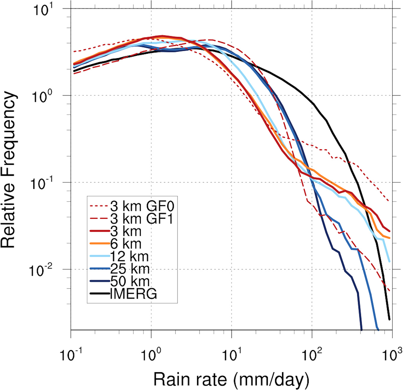
The distribution of precipitation intensity over CONUS is compared with IMERG in Fig. 18, using hourly mean model and IMERG data interpolated to a common 0.5 degree grid for consistency. The model generally overestimates light precipitation, under 5 mm day−1. Simulation of heavier precipitation depends strongly on resolution, with the 25 km and 50 km cases producing more at moderate rates (10 to 100 mm day−1) and higher resolutions producing more above 100 mm day−1. An inflection point is seen around 80 mm day−1 in the 3–12 km curves, likely associated with the reduced parameterized convection in those cases, which allows more convective precipitation from resolved updrafts. The GF0 and GF1 experiments (dashed curves in Fig. 18), show that a 3.5 km run with increased parameterized convection looks similar to the 25 km and 50 km cases, while a 3.5 km run with no parameterized convection has significantly stronger precipitation rates, though it is not necessarily a better match to IMERG.
10. Summary and conclusions
We have evaluated the diurnal cycle of precipitation in a set of non-hydrostatic AGCM simulations with nominal grid spacing ranging from 3.5 km to 50 km. Finer resolution is often expected to improve representation of diurnal variability by reducing reliance on subgrid parameterizations that introduce uncertainty into model formulation. While we do find that some aspects of the diurnal cycle improve with resolution, these improvements are partially offset by degradations in other areas. The results emphasize the complicated and regional nature of the diurnal cycle and the many physical mechanisms that govern it.
In general, we find that amplitudes of the diurnal harmonic appear more similar to the observed multi-year August climatology in the low resolution cases, while the 3.5 km and 6 km cases appear to suffer from excessive small-scale variability. This overproduction of strong small-scale storms has been reported in other studies with explicit convection (Kendon et al. 2012; Hanley et al. 2019), and can be made worse when parameterized convection is removed entirely (Pearson et al. 2014). We find that resolution has no consistent impact on the regional-scale amplitudes, with some regions showing larger amplitude at high resolution (e.g., the western United States and Maritime Continent), and other regions at low resolution (e.g., the southern Amazon).
Over regions where the diurnal cycle is dominated by local thermodynamic forcing, such as over the southeastern United States, precipitation in the higher resolution cases generally peaks several hours earlier than with low resolution, and typically earlier than observations. The delay at low resolution is primarily due to the Grell-Freitas parameterized convection, which employs the non-equilibrium closure of Bechtold et al. 2014. When this closure is disabled, the low resolution precipitation peaks even earlier than the high resolution cases.
Higher resolution generally offers improvement in regions where diurnal variability is dependent on organized propagating convection. Over CONUS, more realistic mesoscale organization enables eastward propagating systems that produce a more realistic nocturnal precipitation peak over the Great Plains, which is largely missing at low resolution. This is consistent with previous studies using regional models over CONUS (e.g., Gao et al. 2017). However, the improvement is not global, or monotonic with resolution. For example, the intensity of propagating rainfall offshore of Sumatra is arguably best in the 6 km simulation (Fig. 10).
We also examined the statistics of convective cloud clusters, identified using a brightness temperature threshold, and their dependence on resolution. We find that at high resolution the intensity of precipitation varies more realistically with convective cluster size, and the diurnal cycle of cloud cluster number better matches observations. On the other hand, while cloud cluster size histograms indicate that coarse resolutions are unable to represent the smallest clusters, the relative number of small cloud clusters becomes overestimated when model grid spacing drops below 12 km. Unlike the excessive small-scale precipitation noted above, this bias actually grows worse with stronger parameterized convection, and instead may be related to issues of upscale convective growth, discussed below.
The role of the Grell-Freitas (GF) parameterization at 3.5 km grid spacing was explicitly examined in “mechanism-denial” experiments, in which the parameterization was either switched off entirely (GF0) or fully enabled by removing its scale-aware throttling function (GF1). The analysis shows that even at 3.5 km, GF produces a diurnal cycle amplitude and phase quite similar to that of the 50 km case. This implies, as argued by Pearson et al. (2014), that differences between the low and high resolution cases are largely driven by scaling of the parameterized convection, rather than changes in resolution itself. The precipitation intensity as a function of cluster size in GF1 similarly resembles the 50 km case, while simultaneously worsening the size distribution bias toward small cloud clusters.
These results highlight the continued importance of model formulation even at convection-permitting resolutions. Some deficiencies in the 3.5 km case, such as the too early diurnal peaks in locally forced regimes, and overestimated small-scale variability, may be associated with insufficient inhibition of resolved updrafts. Many convection-permitting models include an explicit parameterization of horizontal subgrid mixing (e.g., a Smagorinsky-Lilly scheme) that contributes to the dilution of buoyant air in resolved updrafts (Kendon et al. 2012; Hanley et al. 2019), and indeed, diurnal variability can be sensitive to its formulation (Pearson et al. 2014). However, the GEOS model does not currently include any such mixing, and as a consequence explicit convection may be unrealistically vigorous and insensitive to environmental conditions. Incorporating a subgrid mixing scheme should be analogous to increasing the entrainment rate with parameterized convection (Bechtold et al. 2004), with potentially similar impacts on diurnal timing.
Other issues, such as the over-estimated number of small cloud clusters, and weak propagation relative to observations, may be associated with insufficient upscale convective growth. A number of errors may contribute to insufficient growth, including the simulated convective environment (such as inadequate CAPE, shear or moisture), misrepresentation of cold pools, or microphysical issues (Coniglio et al. 2010; Thielen and Gallus 2019). Cold pools, generated by hydrometeor loading and evaporative cooling, are an integral part of MCSs, and may aid more generally in diurnal transitions from shallow to deep convection (Khairoutdinov and Randall 2006; Schlemmer and Hohenegger 2014). An analysis of cold pool statistics in these simulations would be a valuable future study, both as a factor in upscale convective development and as an indicator of problems with microphysics.
While the 3.5 km case with GFDL microphysics does show more realistic eastward propagation over the Great Plains (Fig. 3), the improvement does not extend to the Maritime Continent or Amazonia. That case produces unrealistically small diurnal amplitudes in all three regions, as well as early timing in locally forced regimes, consistent with the hypothesis that that problem is due to insufficient subgrid mixing or another non-microphysical issue. Future research and model development with GEOS will explore these and other issues to achieve a realistic balance of variability and intensity in convective regimes.
Acknowledgments
The authors thank two anonymous reviewers for comments which substantially improved this manuscript. This work was supported by the NASA Modeling, Analysis and Prediction (MAP) program. Computing was provided by the NASA Center for Climate Simulation (NCCS). The model output is available on the NASA data portal: https://portal.nccs.nasa.gov/datashare/DYAMOND/. Public access to the model source code is available at github.com/GEOS-ESM/GEOSgcm.
References
- Arakawa, A., and C.-M. Wu, 2013: A unified representation of deep moist convection in numerical modeling of the atmosphere. Part I. J. Atmos. Sci., 70, 1977-1992.
- Arnold, N. P., and W. M. Putman, 2018: Nonrotating convective self-aggregation in a limited area AGCM. J. Adv. Model. Earth Syst., 10, 1029-1046.
- Bacmeister, J. T., M. J. Suarez, and F. R. Robertson, 2006: Rain reevaporation, boundary layer-convection interactions, and pacific rainfall patterns in an AGCM. J. Atmos. Sci., 63, 3383-3403.
- Bechtold, P., J.-P. Chaboureau, A. Beljaars, A. K. Betts, M. Köhler, M. Miller, and J.-L. Redelsperger, 2004: The simulation of the diurnal cycle of convective precipitation over land in a global model. Quart. J. Roy. Meteor. Soc., 130, 3119-3137.
- Bechtold, P., N. Semane, P. Lopez, J.-P. Chaboureau, A, Beljaars, and N. Bormann, 2014: Representing equilibrium and nonequilibrium convection in large-scale models. J. Atmos. Sci., 71, 734-753.
- Bergman, J. W., and M. L. Salby, 1997: The role of cloud diurnal variations in the time-mean energy budget. J. Climate, 10, 1114-1124.
- Betts, A. K., and C. Jakob, 2002: Evaluation of the diurnal cycle of precipitation, surface thermodynamics, and surface fluxes in the ECMWF model using LBA data. J. Geophys. Res., 107, 8045, doi:10.1029/2001JD000427.
- Borovikov, A., R. Cullather, R. Kovach, J. Marshak, G. Vernieres, Y. Vikhliaev, B. Zhao, and Z. Li, 2019: GEOS-5 seasonal forecast system. Climate Dyn., 53, 7335-7361.
- Brockhaus, P., D. Lüaethi, and C. Schäaer, 2008: Aspects of the diurnal cycle in a regional climate model. Meteor. Z., 17, 433-443.
- Carbone, R. E., J. W. Wilson, T. D. Keenan, and J. M. Hacker, 2000: Tropical island convection in the absence of significant topography. Part I: Life cycle of diurnally forced convection. Mon. Wea. Rev., 10, 3459-3480.
- Carbone, R. E., J. D. Tuttle, D. A. Ahijevych, and S. B. Trier, 2002: Inferences of predictability associated with warm season precipitation episodes. J. Atmos. Sci., 59, 2033-2056.
- Clark, A. J.,W. A. Gallus, Jr., and T.-C. Chen, 2007: Comparison of the diurnal precipitation cycle in convection-resolving and non-convection-resolving mesoscale models. Mon. Wea. Rev., 135, 3456-3473.
- Coniglio, M. C., J. Y. Hwang, and D. J. Stensrud, 2010: Environmental factors in the upscale growth and longevity of MCSs derived from rapid update cycle analyses. Mon. Wea. Rev., 138, 3514-3539.
- Dai, A., and K. Trenberth, 2003: The diurnal cycle and its depiction in the community climate system model. J. Climate, 17, 930-951.
- Del Genio, A. D., 2012: Representing the sensitivity of convective cloud systems to tropospheric humidity in general circulation models. Surv. Geophys., 33, 637-656.
- Del Genio, A. D., and J. Wu, 2010: The role of entrainment in the diurnal cycle of continental convection. J. Climate, 23, 2722-2738.
- Dirmeyer, P. A., B. A. Cash, J. L. Kinter III, T. Jung, L. Marx, M. Satoh, C. Stan, H. Tomita, P. Towers, N. Wedi, D. Achuthavarier, J. M. Adams, E. L. Altshuler, B. Huang, E. K. Jin, and J. Manganello, 2012: Simulating the diurnal cycle of rainfall in global climate models: Resolution versus parameterization. Climate Dyn., 39, 399-418.
- Freitas, S. R., G. A. Grell, A. Molod, M. A. Thompson, W. M. Putman, C. M. Santos e Silva, and E. P. Souza, 2018: Assessing the Grell-Freitas convection parameterization in the NASA GEOS modeling system. J. Adv. Model. Earth Syst., 10, 1266-1289.
- Gao, Y., L. R. Leung, C. Zhao, and S. Hagos, 2017: Sensitivity of U.S. summer precipitation to model resolution and convective parameterizations across gray zone resolutions. J. Geophys. Res.: Atmos., 122, 2714-2733.
- Grabowski W. W., P. Bechtold, A. Cheng, R. Forbes, C. Halliwell, M. Khairoutdinov, S. Lang, T. Nasuno, J. Petch, W.-K. Tao, R. Wong, X. Wu, and K.-M. Xu, 2006: Daytime convective development over land: A model intercomparison based on LBA observations. Quart. J. Roy. Meteor. Soc., 132, 317-344.
- Grell, G. A., and S. R. Freitas, 2014: A scale and aerosol aware stochastic convective parameterization for weather and air quality modeling. Atmos. Chem. Phys., 14, 5233-5250.
- Hanley, K., M. Whitall, A. Stirling, and P. Clark, 2019: Modifications to the representation of subgrid mixing in kilometre-scale versions of the Unified Model. Quart. J. Roy. Meteor. Soc., 145, 3361-3375.
- Huffman, G. J., D. T. Bolvin, E. J. Nelkin, D. B. Wolff, R. F. Adler, G. Gu, Y. Hong, K. P. Bowman, and E. F. Stocker, 2007: The TRMM Multisatellite Precipitation Analysis: Quasi-global, multi-year, combined-sensor precipitation estimates at fine scale. J. Hydrometeor., 8, 38-55.
- Iacono, M. J., J. S. Delamere, E. J. Mlawer, M. W. Shephard, S. A. Clough, and W. D. Collins, 2008: Radiative forcing by long-lived greenhouse gases: Calculations with the AER radiative transfer models. J. Geophys. Res., 113, D13103, doi:10.1029/2008JD009944.
- Janowiak, J. E., R. J. Joyce, and Y. Yarosh, 2001: A real-time global half-hourly pixel-resolution infrared dataset and its applications. Bull. Amer. Meteor. Soc., 82, 205-218.
- Jiang, X., N.-C. Lau, and S. A. Klein, 2006: Role of eastward propagating convection systems in the diurnal cycle and seasonal mean of summertime rainfall over the U.S. Great Plains. Geophys. Res. Lett., 33, L19809, doi:10.1029/2006GL027022.
- Kendon, E. J., N. M. Roberts, C. A. Senior, and M. J. Roberts, 2012: Realism of rainfall in a very high-resolution regional climate model. J. Climate, 25, 5791-5806.
- Khairoutdinov, M., and D. Randall, 2006: High-resolution simulation of shallow-to-deep convection transition over land. J. Atmos. Sci., 63, 3421-3436.
- Koster, R. D., M. J. Suarez, A. Ducharne, M. Stieglitz, and P. Kumar, 2000: A catchment-based approach to modeling land surface processes in a general circulation model: 1. Model structure. J. Geophys. Res., 105, 24809-24822.
- Kuang, Z., and C. S. Bretherton, 2006: A mass-flux scheme view of a high-resolution simulation of a transition from shallow to deep cumulus convection. J. Atmos. Sci., 63, 1895-1909.
- Lee, M.-I., S. D. Schubert, M. J. Suarez, T. L. Bell, and K.-M. Kim, 2007: Diurnal cycle of precipitation in the NASA Seasonal to Interannual Prediction Project atmospheric general circulation model. J. Geophys. Res., 112, D16111, doi:10.1029/2006JD008346.
- Lin, X., D. A. Randall, and L. D. Fowler, 2000: Diurnal variability of the hydrologic cycle and radiative fluxes: Comparisons between observations and a GCM. J. Climate, 13, 4159-4179.
- Lock, A. P., A. R. Brown, M. R. Bush, G. M. Martin, and R. N. B. Smith, 2000: A new boundary layer mixing scheme. Part I: Scheme description and single-column model tests. Mon. Wea. Rev., 128, 3187-3199.
- Loeb, N. G., D. R. Doelling, H. Wang, W. Su, C. Nguyen, J. G. Corbett, L. Liang, C. Mitrescu, F. G. Rose, and S. Kato, 2018: Clouds and the Earth's Radiant Energy System (CERES) Energy Balanced and Filled (EBAF) top-of-atmosphere (TOA) Edition 4.0 Data Product. J. Climate, 31, 895-918.
- Louis, J. F., 1979: A parametric model of vertical eddy fluxes in the atmosphere. Bound.-Layer Meteor., 17, 187-202.
- Love, B. S., A. J. Matthews, and G. M. S. Lister, 2011: The diurnal cycle of precipitation over the Maritime Continent in a high-resolution atmospheric model. Quart. J. Roy. Meteor. Soc., 137, 934-947.
- Mapes, B. E., and R. A. Houze, Jr., 1993: Cloud clusters and superclusters over the oceanic warm pool. Mon. Wea. Rev., 121, 1398-1416.
- Mapes, B. E., T. T. Warner, M. Xu, and A. J. Negri, 2003: Diurnal patterns of rainfall in northwestern South America. Part I: Observations and context. Mon. Wea. Rev., 131, 799-812.
- Moncrieff, M. W., C. Liu, and P. Bogenschutz, 2017: Simulation, modeling, and dynamically based parameterization of organized tropical convection for global climate models. J. Atmos. Sci., 74, 1363-1380.
- Mori, S., J.-I. Harada, Y. I. Tauhid, M. D. Yamanaka, N. Okamoto, F. Murata, N. Sakurai, H. Hashiguchi, and T. Sribimawati, 2004: Diurnal land-sea rainfall peak migration over Sumatra Island, Indonesian Maritime Continent, observed by TRMM satellite and intensive rawinsonde soundings. Mon. Wea. Rev., 132, 2021-2039.
- Neale, R., and J. Slingo, 2003: The Maritime Continent and its role in the global climate: A GCM study. J. Climate, 16, 834-848.
- Park, S., and C. S. Bretherton, 2009: The University of Washington shallow convection and moist turbulence schemes and their impact on climate simulations with the community atmosphere model. J. Climate, 22, 3449-3469.
- Pearson, K. J., R. J. Hogan, R. P. Allan, G. M. S. Lister, and C. E. Holloway, 2010: Evaluation of the model representation of the evolution of convective systems using satellite observations of outgoing longwave radiation. J. Geophys. Res., 115, D20206, doi:10.1029/2010JD014265.
- Pearson, K. J., G. M. S. Lister, C. E. Birch, R. P. Allan, R. J. Hogan, and S. J. Woolnough, 2014: Modelling the diurnal cycle of tropical convection across the grey zone. Quart. J. Roy. Meteor. Soc., 140, 491-499.
- Pritchard, M. S., M. W. Moncrieff, and R. C. Somerville, 2011: Orogenic propagating precipitation systems over the United States in a global climate model with embedded explicit convection. J. Atmos. Sci., 68, 1821-1840.
- Putman, W. M., and S.-J. Lin, 2007: Finite-volume transport on various cubed-sphere grids. J. Comput. Phys., 227, 55-78.
- Putman, W. M., and M. Suarez, 2011: Cloud-system resolving simulations with the NASA Goddard Earth Observing System global atmospheric model (GEOS-5). Geophys. Res. Lett., 38, L16809, doi:10.1029/2011GL048438.
- Rio, C., F. Hourdin, J.-Y. Grandpeix, and J.-P. Lafore, 2009: Shifting the diurnal cycle of parameterized deep convection over land. Geophys. Res. Lett., 36, L07809, doi:10.1029/2008GL036779.
- Ruppert, J. H., X. Chen, and F. Zhang, 2020: Convectively forced diurnal gravity waves in the Maritime Continent. J. Atmos. Sci., 77, 1119-1136.
- Sato, T., H. Miura, M. Satoh, Y. N. Takayabu, and Y. Wang, 2009: Diurnal cycle of precipitation in the tropics simulated in a global cloud-resolving model. J. Climate, 22, 4809-4826.
- Schlemmer, L., and C. Hohenegger, 2014: The formation of wider and deeper clouds as a result of cold-pool dynamics. J. Atmos. Sci., 71, 2842-2858.
- Stevens, B., M. Satoh, L. Auger, J. Biercamp, C. S. Bretherton, X. Chen, P. Düben, F. Judt, M. Khairoutdinov, D. Klocke, C. Kodama, L. Kornblueh, S.-J. Lin, P. Neumann, W. M. Putman, N. Röber, R. Shibuya, B. Vanniere, P. L. Vidale, N. Wedi, and L. Zhou, 2019: DYAMOND: the DYnamics of the Atmospheric general circulation Modeled On Non-hydrostatic Domains. Prog. Earth Planet. Sci., 6, 61, doi:10.1186/s40645-019-0304-z1.
- Stratton, R. A., and A. J. Stirling, 2012: Improving the diurnal cycle of convection in GCMs. Quart. J. Roy. Meteor. Soc., 138, 1121-1134.
- Suhas, E., and G. J. Zhang, 2014: Evaluation of trigger functions for convective parameterization schemes using observations. J. Climate, 27, 7647-7666.
- Tan, J., G. Huffman, D. T. Bolvin, and E. J. Nelkin, 2019: Diurnal cycle of IMERG V06 precipitation. Geophys. Res. Lett., 46, 13584-13592.
- Thielen, J. E., and W. A. Gallus, Jr., 2019: Influences of horizontal grid spacing and microphysics on WRF forecasts of convective morphology evolution for nocturnal MCSs in weakly forced environments. Wea. Forecasting, 34, 1495-1517.
- Wallace, J. M., 1975: Diurnal variations in precipitation and thunderstorm frequency over the conterminous United States. Mon. Wea. Rev., 103, 406-419.
- Wang, Y., L. Zhou, and K. Hamilton, 2007: Effect of convective entrainment/detrainment on the simulation of the tropical precipitation diurnal cycle. Mon. Wea. Rev., 135, 567-585.
- Yang, G.-Y., and J. Slingo, 2001: The diurnal cycle in the tropics. Mon. Wea. Rev., 129, 784-801.
- Zhao, Q., and F. H. Carr, 1997: A prognostic cloud scheme for operational NWP models. Mon. Wea. Rev., 125, 1931-1953.