Abstract
It is speculated that floods in many areas of the world have become more severe with global warming. This study describes the 2017 spring floods in Kazakhstan, which, with about six people dead or missing, prompted the government to call for more than 7,000 people to leave their homes. Then, based on the Climatic Research Unit (CRU), the NCEP/NCAR Reanalysis 1, and the Coupled Model Intercomparison Project 5 (CMIP5) simulations, the seasonal trends of temperature were calculated using the linear least-squares regression and the Mann–Kendall trend test. The correlation between the surface air temperature and atmospheric circulation was explored, and the attributable risk of the 2017 spring floods was evaluated using the conventional fraction of the attributable risk (FAR) method. The results indicate that the north plains of Kazakhstan had a higher (March–April) mean temperature anomaly compared to the south plains, up to 3°C, relative to the 1901–2017 average temperature. This was the primary cause of flooding in Kazakhstan. March and April were the months with a higher increasing trend in temperature from 1901 to 2017 compared with other months. In addition, a positive anomaly of the geopotential height and air temperature for the March–April 2017 period (based on the reference period 1961–1990) was the reason for a warmer abnormal temperature in the northwest region of Kazakhstan. Finally, the FAR value was approximately equal to 1, which supported the claim of a strong anthropogenic influence on the risk of the 2017 March–April floods in Kazakhstan. The results presented provide essential information for a comprehensive understanding of the 2017 spring floods in Kazakhstan and will help government officials identify flooding situations and mitigate damage in future.
1. Introduction
In 2017, a rapid spring thaw caused heavy flooding in the northern and central regions in Kazakhstan (Fig. 1a), which swept away cars, submerged cities, as well as destroyed homes, schools, roads, bridges, and other infrastructure. The flood had about six people dead or missing and prompted the government to call for more than 7,000 people to leave their homes (Davies 2017; RFE/RL's Kazakh Service 2017). These floods were primarily attributed to the rapid increase in temperature in Spring 2017, which caused the rapid melting of snow and ice. The resulting water runoff quickly accumulated, resulting in rivers overflowing their banks and inundating riverside traffic arteries (e.g., railways) and cities and districts, especially Karaganda, Atbasar, Tselinograd, Sandyktau, Aktobe, and Beskaragay (see Fig. 1b).
Kazakhstan, located in Central Asia, is the world's largest landlocked country, the climate of which is typically continental with warm summers and very cold winters (Salnikov et al. 2015). It is highly prone to river floods (Plekhanov 2017), droughts (Zhang, M. et al. 2017), earthquakes (Campbell et al. 2015), and landslides (Havenith et al. 2015). As per the statistics of the Global Emergency Disaster Database (EM-DAT), a significant number of floods occurred (58.8 % of all disasters) during the 1990–2014 period, causing significant casualties, economic losses, and environmental pollution (Heaven et al. 2000; Plekhanov 2017). On the basis of the water regime of rivers in Kazakhstan, all floods could be divided into four types, namely, the Kazakhstan type, Tien Shan type, Altai type, and “No outflow” type (Plekhanov 2017). Kazakhstan type flooding occurred in the steppe and semidesert rivers located in the northwestern, northern, and central regions mainly due to the melting of seasonal snow cover on the plains and low mountain areas. Tien Shan type flooding is typical for rivers (e.g., Syr Darya River) of southeastern and southern Kazakhstan mainly because of the intensive melting of seasonal snow or glacial cover in mountainous areas (Aizen et al. 1996). Altai-type flooding is typical for rivers (e.g., Irtysh River) of the mountain regions of eastern Kazakhstan in which rivers were characterized by spring floods that lasted for 1–2 months. “No outflow”-type flooding happens in small rivers in the central and western desert and semidesert parts of the country mainly due to the strong, intensive rainfalls. It is obvious that considerable melting of seasonal snow and glaciers is the primary reason for flooding in Kazakhstan, which will probably become more frequent and serious under global warming (Pollner et al. 2010). For example, future anthropogenic climate change possibly will lead to (1) additional intense precipitation events (Zhang, M. et al. 2017); (2) accelerated melting of snow and glaciers (Sorg et al. 2012); and (3) increased soil aridity because of high rates of evaporation (Lioubimtseva et al. 2005), resulting in the upper layer of soil washing away more readily. All these changes tend to increase flood losses because of increase in exposure linked to ongoing economic development (Thurman 2011).
The evidence for the impact of climate change on both hydro-climatology and water-related disasters of Kazakhstan is considerable (Salnikov et al. 2015; Shivareva and Bulekbayeva 2017; Zou et al. 2019). The annual bulletin of climate change (issued by the Ministry of Environmental Protection of the Republic of Kazakhstan) indicates that the country's average annual temperature increased by 0.27°C decade−1 during the 1941–2014 period and that the biggest increase, up to 0.38°C decade−1, was detected in spring in the northern, central, and eastern regions. The annual precipitation slightly decreased by 0.8 mm decade−1 from 1941 to 2014 and increased during winter, whereas it decreased during the other three seasons. Furthermore, climate change already increased the frequency of extreme precipitation and temperature over Central Asia (Zhang, R. et al. 2017), thus causing additional water-related disasters in Kazakhstan (Salnikov et al. 2015; Thurman 2011).
Many studies have examined the impact of climate change on global floods (Blöschl et al. 2017; Iwami et al. 2017; Winsemius et al. 2016). Seasonal floods are the norm in many rivers (Wirth et al. 2013), of which spring floods are usually attributed to enough snow accumulation in winter and warm temperatures in spring (Prowse et al. 2010). Heavy snow accumulation in many parts of the middle- to high-latitude regions indicates an increased risk of flooding if the weather turns to spring too quickly (Frolova et al. 2015; Mazouz et al. 2012), which has become increasingly common under climate change (Blöschl et al. 2019; Veijalainen et al. 2010). However, only a few relevant studies examined the causes and contributors to spring floods in Kazakhstan, especially for the investigation of temperature.
Therefore, the aim of this study is (1) to investigate the changes in the March–April temperature in Kazakhstan from 1901 to 2017 because the increasing temperature was the primary driver for the 2017 spring floods; (2) to evaluate the relation between the warming temperature and atmospheric circulation; and (3) to explore how human-induced climate change causes a warmer temperature and increased spring flood events in Kazakhstan. This study is structured as follows: the datasets and methods are briefly described in Section 2. The results of changes in temperature, correlation analysis, and contribution analysis are elaborated in Section 3, followed by the conclusions in Section 4.
2. Datasets and methods
2.1 Datasets
In Central Asia, because of the lack of long-term ground-based observation data, the Climatic Research Unit (CRU, TS v.4.03) was used to calculate the monthly, seasonal, and yearly temperature and precipitation in Kazakhstan from 1901 to 2018. In May 2019, this dataset was produced and issued by CRU at the University of East Anglia, England, with a resolution of 0.5° × 0.5° and using the same method as for an earlier version (Harris et al. 2014). Furthermore, the CRU dataset has been extensively used in many previous studies (Nakaegawa et al. 2015) and has been confirmed to be reasonable for Central Asia (Malsy et al. 2015; Zou et al. 2019).
To fully understand the atmospheric processes leading to the 2017 spring floods in Kazakhstan, the data of the NCEP/NCAR Reanalysis 1 (Kalnay et al. 1996) were used to understand the large-scale atmospheric circulation from the surface to upper layers. On the basis of the data from 1948 to present, a state-of-the-art analysis/forecast system was used to perform data assimilation in the NCEP/NCAR Reanalysis 1 project, which has been extensively applied in multiple studies (Basu and Sauchyn 2019; Romanic et al. 2018). In this study, parameters, including the air temperature, geopotential height, and wind, were used to evaluate the relation between atmospheric circulation and 2017 spring floods.
To assess the contribution of human influence on increase in temperature in Kazakhstan, temperature simulations from about 40 global climate models (GCMs) from the Coupled Model Intercomparison Project Phase 5 (CMIP5; see Taylor et al. 2012) were employed. These CMIP5 models provided 13 temperature simulations (one member run “r1i1p1”) with a preindustrial control setting, natural forcing only (NAT), and all forcing (ALL). Then, two evaluation methods were applied to identify and select models. One is the positive spatial correlation coefficient for the interannual March–April mean temperature between the CRU and the CMIP5 ALL simulations in Kazakhstan. Furthermore, the criterion is that the coefficient should be larger than or equal to 0. The other method is the Kolmogorov–Smirnov (K–S) test (Nakaegawa and Kanamitsu 2006; Nakaegawa and Nakakita 2012) between the CRU and the CIMP5 ALL simulations; the p value should be < 0.05. Finally, 10 models were selected to analyze the attribution (Table 1). For each CMIP5 model, only one member run (“r1i1p1”) was employed. The ALL simulations of most models ended in 2005. To compare the observations from 1961 to 2017 better, the March–April annual mean temperature projections from the Representative Concentration Pathways 8.5 (RCP8.5) scenario were used to extend the time series of ALL simulations through 2017 based on the method proposed by Zhou et al. (2014).

Linear least-squares regression (Hess et al. 2001) was applied to estimate the trend of the monthly and yearly temperatures at the grid and the national scales for Kazakhstan, and their significance in each time series was evaluated using the Mann–Kendall trend test (Kendall 1975). The national temperature time series were calculated from the average of all grid points.
To understand the temperature variations in different subperiods better, we divided the period into four subperiods, namely, 1901–1930, 1931–1960, 1961–1990, and 1991–2017, as well as calculated the probability distribution functions for the March–April annual mean temperature for all four subperiods.
When evaluating the contribution of the human influence on the increasing temperature in Kazakhstan, three temperature indices were measured namely, TNn (monthly minimum value of the daily minimum temperature), TXx (monthly maximum value of the daily maximum temperature), and the mean temperature.
The conventional fraction of the attributable risk (FAR) method was used to quantify the attributable risk of the 2017 spring floods in the model analysis (Stone and Allen 2005; Stott et al. 2004). The FAR value could be calculated using the following equation:
where
FAR is the fraction of the risk for the occurrence of the 2017 spring floods in Kazakhstan that is attributed to the inclusion of additional forcing from one scenario to the next,
PALL is the probability of the event under ALL forcing, and
PNAT is the probability under the NAT forcing. Both
PALL and
PNAT could be computed based on the CMIP5 ALL and NAT simulations. Based on the definition of the calculating process of
FAR and the CMIP5 ALL and NAT simulations, we first compared the real temperature and ALL and NAT simulations, and then calculated
PALL and
PNAT. The
FAR values provide a quantification of the change in probability of the defined event occurring (here, the occurrence of the 2017 spring floods in Kazakhstan) that can be attributed to a particular cause, particularly the difference between model experiments (i.e., anthropogenic climate forcings). For instance, a value of
FAR = 0.5 suggests that the risk of an extreme event is doubled over natural conditions because of the anthropogenic climate change. Because of the lack of the observed TXx and TNn, we only compared the probability of the observed 2017 March–April mean temperature occurring in the ALL forcing (
PALL) and the NAT forcing (
PNAT) simulations to determine the contribution of anthropogenic climate change.
Furthermore, to estimate the FAR uncertainty, the bootstrapping method (with replacement) was applied in this CMIP5-based study. For determining the FAR values associated with the 2017 March–April mean temperatures in Kazakhstan, each distribution of temperature was bootstrap resampled 1,000 times (using in each iteration subsamples of all years from only 50 % of available model simulations) to produce a distribution of FAR values (Lewis and Karoly 2013). This distribution of 1000 FAR values represents the uncertainty associated using different models and provides a basis for communicating FAR ranges. In this study, e.g., both the median and 10th percentile FAR values indicate that they are exceeded by 90 % of values in the bootstrapped FAR distributions; moreover, they can be described as “best estimate” and “very likely” values, respectively.
3. Results and discussions
3.1 Changes in temperature
Figure 2a shows the distribution of mean temperature in the March–April 2017 period (Kazakhstan), suggesting that the temperature was high in most regions except for northern Kazakhstan and high mountains. The south plains had a higher temperature than the north plains; moreover, both Tien Shan and Altai Mountains showed a lower temperature than other plains. However, the north plains had a higher mean temperature anomaly (up to 3°C) in March–April than the south plains compared to the average temperature in 1901–2017 (Fig. 2b), which shows that abnormally high temperatures appeared in spring 2017 and probably accelerated the snow and ice melting in Kazakhstan. The unusually warm temperatures engulfed a large part of Kazakhstan in March–April 2017, which agreed with the trend of mean temperature in March–April from 1901 to 2017 (Figs. 2c, d).

Figure 2c also clearly illustrates that all grids in Kazakhstan exhibited positive trends at the 95 % confidence level and that the southern regions had lower trends than the northern regions. Figure 2d shows that a significant, increasing trend at 0.25°C decade−1 was detected during the 1901–2017 period for the entire Kazakhstan; moreover, the national mean temperature in March–April was greater than 7.50°C since 2004. Of those, the most notable warm temperature anomalies were present across most of Kazakhstan during March and April 2008, up to 6.77°C, and the value amounted to 3.41°C in 2017. All these springs (with a warm temperature anomaly) had floods in the warm temperature and dramatically accelerated the snow melting and ice disintegration in early spring. Figure 2e shows the bivariate return periods for the current March–April mean temperature, which suggests that the 2017 March–April warm temperature was close to a 1-in-6-year event. Figure 2f shows that the March–April temperature demonstrated a positive shift from the first time (1901–1930) to the fourth time period (1991–2017), suggesting that the warm temperature anomaly has increasingly become common and significant (the right tail of each time period). The increasing trend in temperature is consistent with the analysis from Pilifosova et al. (1997) and Salnikov et al. (2015).
Furthermore, Fig. 2d shows that certain other years had higher mean temperatures in March–April compared with that in March–April in 2017. For example, the national mean temperature was greater than 10°C in March–April 2008, which was considerably higher than that in March–April 2017. However, the warm temperature in 2008 did not cause more floods than in 2017 because there was not enough snow accumulation during this year. More concretely, there was additional winter precipitation in 2017 over Kazakhstan (Fig. 2g), and precipitation anomaly was greater than 10 mm in northern regions (Fig. 2h). Figure 2i shows the spatial distribution of differences of winter precipitation between 2008 and 2017, which suggests that winter precipitation in 2017 was considerably higher than that in 2008; furthermore, the largest difference value was up to 20 mm in the northern regions of Kazakhstan.
To compare temperature variations between March–April and the other months, the monthly temperature was analyzed. Figure 3 shows the mean monthly temperature in Kazakhstan from 1901 to 2017, which shows that July had the highest mean temperature (approximately 23.14°C), whereas January had the lowest (approximately −12.55°C). The mean temperature was greater than 0°C in April, May, June, July, August, September, and October; however, it was negative in November, December, January, February, and March. Of those, the temperature during March and April is extremely important for determining the spring melting and snow cover (see blue box plots in Fig. 3b). For example, the increasing temperature could cause earlier spring melting and reduced snow cover seasons and vice versa. Uneven spatial distributions are also found in Fig. 3a. Generally, the southern regions have a higher temperature than northern regions, and the temperature is greater than 30°C in the southern regions in summer but less than −30°C in the northern regions in summer.

Figure 4 shows the trends of mean monthly temperature in Kazakhstan from 1901 to 2017, which shows that an increase was detected for all months ranging from 0.06°C to 0.37°C decade−1. Note that July had the lowest trend for the mean temperature (approximately 0.06°C decade−1), whereas March had the highest trend for the mean temperature (approximately 0.37°C decade−1), followed by April (approximately 0.26°C decade−1) and February (approximately 0.22°C decade−1). Obviously, in these two months, the increase in (both March and April) temperature had significantly uplifted the mean temperature (see Fig. 3), probably causing earlier spring melting and shorter snow cover seasons (Kaldybayev et al. 2016; Kitaev et al. 2005). Moreover, Fig. 4 shows that an uneven spatial distribution was detected for all months. The north had higher trends than the south in March and April, and the largest increase amounted to 0.5°C decade−1 in the north fringe in Kazakhstan. The northern regions had higher trends than the southern regions in March and April, and the largest increase was more than 0.5°C decade−1 in the north fringe regions in Kazakhstan; however, in July and September, the southern regions had higher trends than the northern regions, and the lowest increase was reported in the north fringe regions in Kazakhstan, up to 0°C decade−1.

Generally, the anomalies of synoptic conditions have been confirmed to contribute to extreme temperature and precipitation events (Lau and Kim 2012; Milrad et al. 2015), particularly under climate change. Therefore, to investigate the characteristics of flood occurrence in Kazakhstan, composite analysis was calculated and contoured for the following atmospheric variables in the data of the NCEP/NCAR Reanalysis 1: 500 hPa and 850 hPa air temperature, geopotential height, and wind. Figure 5 shows the contour maps of the anomalies in air temperature, geopotential height, and wind vector at 500 hPa and 850 hPa from March to April 2017 (based on the 1961–1990 reference period).
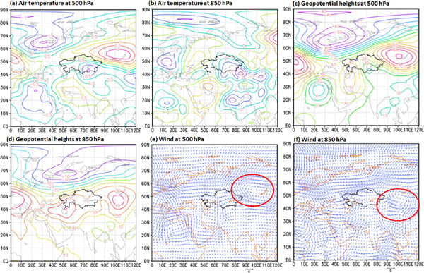
As can be seen from Figs. 5a and 5b, a positive air temperature anomaly was detected in the northwest and northeast regions at both 500 hPa and 850 hPa but a negative one in the southeast mountains. The anomalies of air temperature at 500 hPa show that the largest anomaly was up to +1°C in the northern regions, which probably accelerated ice melting and caused a series of floods in the northern regions of Kazakhstan because there are multiple small river networks in these areas (see Fig. 1). Figure 5c shows that the March–April 2017 period was characterized by a strong positive geopotential anomaly at 500 hPa, based on the 1961–1990 reference period of ∼ 30 gpm with a maximum (larger than 40 gpm) in the northwest region and a minimum (less than 20 gpm) in the southeast corner of Kazakhstan. Moreover, Fig. 5c shows a blocking high in the east of Kazakhstan, which may be the main cause of high temperatures in Kazakhstan. The 850 hPa geopotential anomaly reached about 20 gpm with a maximum (more than 30 gpm) in the southwest corner (Fig. 5d). Compared with Figs. 5a and 5c, the occurrence of warm spring in Kazakhstan was accompanied by a positive anomaly at 500 hPa. Moreover, large positive anomalies at 500 hPa played an important role in maintaining prolonged extreme temperature spells and atmospheric blocking (Tomczyk et al. 2017). Furthermore, Figs. 5e and 5f show anomalies of the wind vector at 500 hPa and 850 hPa (m s−1) in March–April 2017, thus revealing an anticyclonic system in eastern Kazakhstan for both pressure layers.
Figure 6 shows that the anomalies of the geopotential height and air temperature were calculated and contoured in the vertical cross-sections of the troposphere. Generally, the occurrence of the anomalies in the March–April 2017 period was related to the positive anomalies of geopotential height on all isobaric levels (100–1000 hPa) throughout the troposphere. On the basis of the 1961–1990 reference period, the largest anomalies of geopotential heights occurred at the level of ∼ 250 hPa, with the maximum along the meridian of 100°E (> 120 gpm) (Fig. 6d). Figure 6d also shows that the positive air temperature anomalies occurred with the highest values exceeding 4°C on the 1000–750 hPa geopotential levels. Moreover, in Figs. 6a and 6b (40°N, 45°N), there were negative air temperature anomalies from 60°E to 80°E in the lower troposphere (below the level of 300 hPa) probably because most of these regions are high mountains and the surface air temperature is extremely low. In the upper troposphere (above the level of 200 hPa), however, there were negative air temperature anomalies in Figs. 6c and 6d (50°N, 55°N), which shows a characteristic circulation of air masses within high-pressure areas. That is, the horizontal convergence of air masses in the upper part of the high-pressure area causes adiabatic cooling, leading to negative air temperature anomalies, whereas the positive anomalies in its lower part are a consequence of the settlement of air masses activating adiabatic heating (Tomczyk 2018).

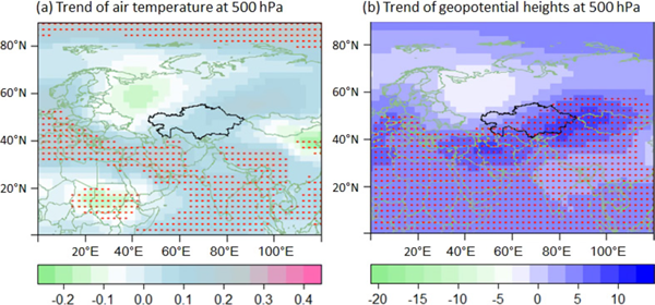
The spatial patterns of the 1948–2017 trends constructed with air temperature and geopotential height at 500 hPa are plotted in Fig. 7, suggesting an increasing trend over Kazakhstan. The trends both show an overall increase at 500 hPa and display negative trends in certain regions for both air temperature and geopotential height. The spatial patterns of trends may trigger a dynamical climatic response via changes in circulation, whereas increased geopotential height at 500 hPa may contribute to the occurrence of warm spells weather through direct and indirect effects (Black et al. 2004; Freychet et al. 2017). Here, the relative increase in geopotential height at 500 hPa around Kazakhstan (Fig. 7b) may enhance the downward solar radiation and subsidence warming and moderate cold flow from the Siberia and the Arctic Ocean, which consequently increased the surface air temperature.
From the above analysis, therefore, we can possibly conclude that the northeastward shift of the anticyclonic high-pressure system reduced the northerly wind transporting cold air from the Siberia and the Arctic Ocean to Kazakhstan, thus favoring a positive air temperature anomaly. The result is consistent with the interdecadal variation in the Central Asia pattern from Yu et al. (2019): that is, a positive 500-hPa height anomalies and an anomalous anticyclonic circulation over the northwest of the region, corresponding to the increasing occurrence of warm spells weather in Central Asia.
3.3 Contribution analysis
To conduct the attribution analysis of the 2017 spring floods in Kazakhstan, we calculated and compared the probability of the event occurrence under the CMIP5 ALL and NAT simulations. Figure 8 shows the kernel curves of the TNn, TXx, and the mean temperature for CMIP5 ALL and NAT simulations.
As shown in Fig. 8a, the TNn probability density curves shifted to the right from the NAT simulations to ALL simulations with a corresponding mean value at −18.47°C and −17.99°C, respectively, which suggests an increase in the mean value of the TNn and a decrease in the occurrence of cold weather in spring in Kazakhstan. Similarly, the March–April TXx probability density curves (Fig. 8b) shifted to the right from NAT simulations to ALL simulations with a corresponding mean value at 22.72°C and 22.96°C, respectively. This indicates an augmentation in the occurrence of hot weather in spring in Kazakhstan under the influence of anthropogenic forcing.
Similar to the case of TNn and TXx, the probability density curves regarding the mean temperature in March–April tended to shift from the NAT distributions to the right direction in ALL simulations with a corresponding mean value at 2.34°C and 2.43°C, respectively, which indicates that the average temperature increased by 0.09°C because of the natural forcing. Correspondingly, the contribution of the anthropogenic forcing to the observed spring floods 2017 in Kazakhstan was 100 % (FAR = 1, Fig. 8c), thus supporting the claim of a strong anthropogenic influence on these floods.
Furthermore, we note that although CMIP5 models' outputs are suitable for estimating FAR, the FAR values are arguably uncertain because of the complexity of extreme climate events and the intrinsic uncertainty that arises from model deficiencies (Bellprat and Doblas Reyes 2016; National Academies of Sciences, Engineering, and Medicine 2016). To reduce uncertainties from the limitations of climate model resolution and erroneous representation relevant physical mechanisms, previous studies have to date attempted to use multimodel ensembles (Duan et al. 2019; Fischer and Knutti 2015) or multimethod approaches (Otto et al. 2015). However, unreliable climate models are still prone to overestimating FAR because of overconfident ensemble spread and model deficiencies; furthermore, the FAR may affect the interannual and decadal variabilities with different phases in different model simulations (Bellprat and Doblas Reyes 2016; National Academies of Sciences, Engineering, and Medicine 2016; Slingo and Palmer 2011). Therefore, contribution studies in future should increasingly consider model correction approaches and larger ensembles to reduce sampling uncertainty and account for model uncertainties, respectively (Bellprat and Doblas Reyes 2016; Otto et al. 2016).
4. Conclusions
In this study, the spring floods in Kazakhstan were first described in 2017, which indicates that a rapid spring thaw caused heavy flooding in the northern and central regions in Kazakhstan, resulting in rivers overflowing their banks and inundating the riverside cities. Then, on the basis of the CRU datasets and NCEP/NCAR Reanalysis 1, the trends of monthly and yearly temperatures at the grid and national scales (for Kazakhstan) were calculated; moreover, their correlation with the atmospheric circulation was assessed. The contribution from the influence of the anthropogenic force was estimated by calculating three temperature indices, namely, TXx, TNn, and mean temperature, for the CIMP5 NAT and ALL simulations. The results could be summarized as follows:
(1) The warmer abnormal temperature in March–April 2017 was the primary cause of flooding in Kazakhstan. The north plains had a higher March–April mean temperature anomaly compared to southern regions, up to 3°C, relative to the 1901–2017 average temperatures, thus accelerating the snow and ice melting in Kazakhstan, which was consistent with the trend of the mean March–April temperature during the 1901–2017 period. Compared with other months, both March and April demonstrated a higher trend from 1901 to 2017, with the value at approximately 0.37°C decade−1 and 0.26°C decade−1, respectively. This probably caused earlier spring melting and shorter snow cover seasons.
(2) A blocking high in the east of Kazakhstan directly caused a positive anomaly of the geopotential height and air temperature in the March–April 2017 period (based on the reference period 1961–1990), eventually leading to a warmer abnormal spring temperature in Kazakhstan. The largest geopotential height and air temperature anomalies at both 500 hPa and 850 hPa were up to 40 gpm and +1°C, respectively, in the northwestern part of Kazakhstan. This explained why the warmer abnormal temperature in the northwest region was higher than that in the southeast region. Moreover, the northeastward shift of the anticyclonic high-pressure system reduced the northerly wind transporting cold air from the Siberia and Arctic Ocean to Kazakhstan, thus favoring a positive air temperature anomaly.
(3) The attribution analysis indicated that the risk of the 2017 March–April floods in Kazakhstan could be attributed to anthropogenic forcing. The kernel curves of the March–April TNn, TXx, and mean temperature shifted to the right from the CMIP5 NAT simulations to the CMIP5 ALL simulations. Moreover, the contribution of anthropogenic forcing to the observed 2017 spring floods in Kazakhstan was 100 % (FAR = 1), thus supporting the claim of a strong anthropogenic influence on 2017 spring floods. However, additional contribution studies should increasingly consider model correction approaches and larger ensembles to reduce sampling uncertainty and account for model uncertainties, respectively.
Acknowledgments
This study is sponsored by the National Natural Science Foundation of China (No. 41971149), the National Natural Science Foundation of China (U1603242), the Key Research Program of the Chinese Academy of Sciences (ZDRWZS-2019-3), the Program for High-Level Talents Introduction in Xinjiang Uygur Autonomous Region (Y941181), and the Chinese Academy of Sciences President's International Fellowship Initiative (Grant No. 2017VCA0002). We also thank Sabine CNUDDE for improving the language. The first author would like to thank the China Scholarship Council for her PhD scholarships.
The authors declare that they have no conflicts of interest.
References
- Aizen, V. B., E. M. Aizen, and J. M. Melack, 1996: Precipitation, melt and runoff in the northern Tien Shan. J. Hydrol., 186, 229-251.
- Basu, S., and D. Sauchyn, 2019: An unusual cold February 2019 in Saskatchewan—A case study using NCEP reanalysis datasets. Climate, 7, 87; doi:10.3390/cli7070087.
- Bellprat, O., and F. Doblas-Reyes, 2016: Attribution of extreme weather and climate events overestimated by unreliable climate simulations. Geophys. Res. Lett., 43, 2158-2164.
- Black, E., M. Blackburn, G. Harrison, B. Hoskins, and J. Methven, 2004: Factors contributing to the summer 2003 European heatwave. Weather, 59, 217-223.
- Blöschl, G., J. Hall, J. Parajka, R. A. P. Perdigão, B. Merz, B. Arheimer, G. T. Aronica, A. Bilibashi, O. Bonacci, M. Borga, I. Čanjevac, A. Castellarin, G. B. Chirico, P. Claps, K. Fiala, N. Frolova, L. Gorbachova, A. Gül, J. Hannaford, S. Harrigan, M. Kireeva, A. Kiss, T. R. Kjeldsen, S. Kohnová, J. J. Koskela, O. Ledvinka, N. Macdonald, M. Mavrova-Guirguinova, L. Mediero, R. Merz, P. Molnar, A. Montanari, C. Murphy, M. Osuch, V. Ovcharuk, I. Radevski, M. Rogger, J. L. Salinas, E. Sauquet, M. Šraj, J. Szolgay, A. Viglione, E. Volpi, D. Wilson, K. Zaimi, and N. Živković, 2017: Changing climate shifts timing of European floods. Science, 357, 588-590.
- Blöschl, G., J. Hall, A. Viglione, R. A. P. Perdigão, J. Parajka, B. Merz, D. Lun, B. Arheimer, G. T. Aronica, A. Bilibashi, M. Boháč, O. Bonacci, M. Borga, I. Čanjevac, A. Castellarin, G. B. Chirico, P. Claps, N. Frolova, D. Ganora, L. Gorbachova, A. Gül, J. Hannaford, S. Harrigan, M. Kireeva, A. Kiss, T. R. Kjeldsen, S. Kohnová, J. J. Koskela, O. Ledvinka, N. Macdonald, M. Mavrova-Guirguinova, L. Mediero, R. Merz, P. Molnar, A. Montanari, C. Murphy, M. Osuch, V. Ovcharuk, I. Radevski, J. L. Salinas, E. Sauquet, M. Šraj, J. Szolgay, E. Volpi, D. Wilson, K. Zaimi, and N. Živković, 2019: Changing climate both increases and decreases European river floods. Nature, 573, 108-111.
- Brakenridge, G. R., and A. J. Kettner, 2017: DFO Flood Event 4465. Dartmouth Flood Observatory, University of Colorado, Boulder, Colorado, USA. [Available at https://floodobservatory.colorado.edu/Events/2017Kazakhstan4465/2017Kazakhstan4465.html.]
- Campbell, G. E., R. T. Walker, K. Abdrakhmatov, J. Jackson, J. R. Elliott, D. Mackenzie, T. Middleton, and J.-L. Schwenninger, 2015: Great earthquakes in low strain rate continental interiors: An example from SE Kazakhstan. J. Geophys. Res.: Solid Earth, 120, 5507-5534.
- Davies, R., 2017: Kazakhstan—7,000 evacuated after snowmelt causes floods in 7 regions. Flood List. [Available at http://floodlist.com/asia/kazakhstan-snowmeltfloods-april-2017.]
- Duan, W., N. Hanasaki, H. Shiogama, Y. Chen, S. Zou, D. Nover, B. Zhou, and Y. Wang, 2019: Evaluation and future projection of Chinese precipitation extremes using large ensemble high-resolution climate simulations. J. Climate, 32, 2169-2183.
- Fischer, E. M., and R. Knutti, 2015: Anthropogenic contribution to global occurrence of heavy-precipitation and high-temperature extremes. Nat. Climate Change, 5, 560-564.
- Freychet, N., S. Tett, J. Wang, and G. Hegerl, 2017: Summer heat waves over eastern China: Dynamical processes and trend attribution. Environ. Res. Lett., 12, 024015, doi:10.1088/1748-9326/aa5ba3.
- Frolova, N. L., S. A. Agafonova, I. N. Krylenko, and A. S. Zavadsky, 2015: An assessment of danger during spring floods and ice jams in the north of European Russia. Proc. Int. Assoc. Hydrol. Sci., 369, 37-41.
- Harris, I., P. D. Jones, T. J. Osborn, and D. H. Lister, 2014: Updated high-resolution grids of monthly climatic observations—The CRU TS3.10 Dataset. Int. J. Climatol., 34, 623-642.
- Havenith, H. B., A. Strom, I. Torgoev, A. Torgoev, L. Lamair, A. Ischuk, and K. Abdrakhmatov, 2015: Tien Shan geohazards database: Earthquakes and landslides. Geomorphology, 249, 16-31.
- Heaven, S., M. A. Ilyushchenko, I. M. Kamberov, M. I. Politikov, T. W. Tanton, S. M. Ullrich, and E. P. Yanin, 2000: Mercury in the River Nura and its floodplain, Central Kazakhstan: II. Floodplain soils and riverbank silt deposits. Sci. Total Environ., 260, 45-55.
- Hess, A., H. Iyer, and W. Malm, 2001: Linear trend analysis: A comparison of methods. Atmos. Environ., 35, 5211-5222.
- Iwami, Y., A. Hasegawa, M. Miyamoto, S. Kudo, Y. Yamazaki, T. Ushiyama, and T. Koike, 2017: Comparative study on climate change impact on precipitation and floods in Asian river basins. Hydrol. Res. Lett., 11, 24-30.
- Kaldybayev, A., Y. Chen, G. Issanova, H. Wang, and L. Mahmudova, 2016: Runoff response to the glacier shrinkage in the Karatal river basin, Kazakhstan. Arabian J. Geosci., 9, 208, doi:10.1007/s12517-015-2106-y.
- Kalnay, E., M. Kanamitsu, R. Kistler, W. Collins, D. Deaven, L. Gandin, M. Iredell, S. Saha, G. White, J. Woollen, Y. Zhu, M. Chelliah, W. Ebisuzaki, W. Higgins, J. Janowiak, K. C. Mo, C. Ropelewski, J. Wang, A. Leetmaa, R. Reynolds, R. Jenne, and D. Joseph, 1996: The NCEP/NCAR 40-year reanalysis project. Bull. Amer. Meteor. Soc., 77, 437-472.
- Kendall, M. G., 1975: Rank Correlation Methods. 4th Edition. Charles Griffin, London.
- Kimoto, M., and M. Ghil, 1993: Multiple flow regimes in the Northern Hemisphere winter. Part I: Methodology and hemispheric regimes. J. Atmos. Sci., 50, 2625-2644.
- Kitaev, L., E. Førland, V. Razuvaev, O. E. Tveito and O. Krueger, 2005: Distribution of snow cover over Northern Eurasia. Hydrol. Res., 36, 311-319.
- Lau, W. K. M., and K.-M. Kim, 2012: The 2010 Pakistan flood and Russian heat wave: Teleconnection of hydrometeorological extremes. J. Hydrometeor., 13, 392-403.
- Lewis, S. C., and D. J. Karoly, 2013: Anthropogenic contributions to Australia's record summer temperatures of 2013. Geophys. Res. Lett., 40, 3705-3709.
- Lioubimtseva, E., R. Cole, J. M. Adams, and G. Kapustin, 2005: Impacts of climate and land-cover changes in arid lands of Central Asia. J. Arid Environ., 62, 285-308.
- Malsy, M., T. aus der Beek, and M. Flörke, 2015: Evaluation of large-scale precipitation data sets for water resources modelling in Central Asia. Environ. Earth Sci., 73, 787-799.
- Mazouz, R., A. A. Assani, J.-F. Quessy, and G. Légaré, 2012: Comparison of the interannual variability of spring heavy floods characteristics of tributaries of the St. Lawrence River in Quebec (Canada). Adv. Water Resour., 35, 110-120.
- Milrad, S. M., J. R. Gyakum, and E. H. Atallah, 2015: A meteorological analysis of the 2013 Alberta flood: Antecedent large-scale flow pattern and synoptic-dynamic characteristics. Mon. Wea. Rev., 143, 2817-2841.
- Nakaegawa, T., and M. Kanamitsu, 2006: Changes in the probability density function of 500-hPa geopotential heights during El Niño and La Niña events. Pap. Meteor. Geophys., 56, 25-33.
- Nakaegawa, T., and E. Nakakita, 2012: Comment on “Effect of uncertainty in temperature and precipitation inputs and spatial resolution on the crop model” by Kenichi Tatsumi, Yosuke Yamashiki and Kaoru Takara. Hydrol. Res. Lett., 6, 13-14.
- Nakaegawa, T., S. Horiuchi, and H. Kim, 2015: Development of a web application for examining climate data of global lake basins: CGLB. Hydrol. Res. Lett., 9, 125-132.
- National Academies of Sciences, Engineering, and Medicine, 2016: Attribution of Extreme Weather Events in the Context of Climate Change. The National Academies Press, 186 pp.
- Otto, F. E. L., K. Haustein, P. Uhe, C. A. S. Coelho, J. A. Aravequia, W. Almeida, A. King, E. Coughlan de Perez, Y. Wada, G. J. van Oldenborgh, R. Haarsma, M. van Aalst, and H. Cullen, 2015: Factors other than climate change, main drivers of 2014/15 water shortage in southeast Brazil. Bull. Amer. Meteor. Soc., 96, S35-S40.
- Otto, F. E. L., G. J. van Oldenborgh, J. Eden, P. A. Stott, D. J. Karoly, and M. R. Allen, 2016: The attribution question. Nat. Climate Change, 6, 813-816.
- Pilifosova, O. V., I. B. Eserkepova, and S. A. Dolgih, 1997: Regional climate change scenarios under global warming in Kazakhstan. Climatic Change, 36, 23-40.
- Plekhanov, P. A., 2017: Natural hydrological risks and their prevention in Kazakhstan. Central Asian J. Water Res., 3, 17-23.
- Pollner, J., J. Kryspin-Watson, and S. Nieuwejaar, 2010: Disaster Risk Management and Climate Change Adaptation in Europe and Central Asia. World Bank, Washington, DC, USA, 54 pp.
- Prowse, T., R. Shrestha, B. Bonsal, and Y. Dibike, 2010: Changing spring air-temperature gradients along large northern rivers: Implications for severity of river-ice floods. Geophys. Res. Lett., 37, L19706, doi:10.1029/2010GL044878.
- RFE/RL's Kazakh Service, 2017: Heavy floods cause damage, spark anger in northern Kazakhstan. Radio Free Europe/Radio Liberty. [Available at http://www.rferl.org/a/kazakhstan-floods-damage-anger/28441118.html.]
- Romanic, D., H. Hangan, and M. Ćurić, 2018: Wind climatology of Toronto based on the NCEP/NCAR reanalysis 1 data and its potential relation to solar activity. Theor. Appl. Climatol., 131, 827-843.
- Salnikov, V., G. Turulina, S. Polyakova, Y. Petrova, and A. Skakova, 2015: Climate change in Kazakhstan during the past 70 years. Quat. Int., 358, 77-82.
- Shivareva, S., and L. Bulekbayeva, 2017: The regional and national best practices for minimizing the risks of water- related disasters in Central Asia—The cross-sectoral working groups in Kazakhstan and Kyrgyzstan. Central Asian J. Water Res., 3, 6-12.
- Slingo, J., and T. Palmer, 2011: Uncertainty in weather and climate prediction. Philos. Trans. Roy. Soc. A, 369, 4751-4767.
- Sorg, A., T. Bolch, M. Stoffel, O. Solomina, and M. Beniston, 2012: Climate change impacts on glaciers and runoff in Tien Shan (Central Asia). Nat. Climate Change, 2, 725-731.
- Stone, D. A., and M. R. Allen, 2005: The end-to-end attribution problem: From emissions to impacts. Climatic Change, 71, 303-318.
- Stott, P. A., D. A. Stone, and M. R. Allen, 2004: Human contribution to the European heatwave of 2003. Nature, 432, 610-614.
- Taylor, K. E., R. J. Stouffer, and G. A. Meehl, 2012: An overview of CMIP5 and the experiment design. Bull. Amer. Meteor. Soc., 93, 485-498.
- Thurman, M., 2011: Natural disaster risks in Central Asia: A synthesis. Bureau for Crisis Prevention and Recovery–UNDP (BCPR-UNDP), 47 pp. [Available at http://www.undp.org/content/dam/rbec/docs/Natural-disasterrisks-in-Central-Asia-A-synthesis.pdf.]
- Tomczyk, A. M., 2018: Impact of atmospheric circulation on the occurrence of hot nights in Central Europe. Atmosphere, 9, 474, doi:10.3390/atmos9120474.
- Tomczyk, A. M., M. Półrolniczak, and E. Bednorz, 2017: Circulation conditions’ effect on the occurrence of heat waves in western and southwestern Europe. Atmosphere, 8, 31, doi:10.3390/atmos8020031.
- Veijalainen, N., E. Lotsari, P. Alho, B. Vehviläinen, and J. Käyhkö, 2010: National scale assessment of climate change impacts on flooding in Finland. J. Hydrol., 391, 333-350.
- Winsemius, H. C., J. C. J. H. Aerts, L. P. H. van Beek, M. F. P. Bierkens, A. Bouwman, B. Jongman, J. C. J. Kwadijk, W. Ligtvoet, P. L. Lucas, D. P. van Vuuren, and P. J. Ward, 2016: Global drivers of future river flood risk. Nat. Climate Change, 6, 381-385.
- Wirth, S. B., A. Gilli, A. Simonneau, D. Ariztegui, B. Vannière, L. Glur, E. Chapron, M. Magny, and F. S. Anselmetti, 2013: A 2000 year long seasonal record of floods in the southern European Alps. Geophys. Res. Lett., 40, 4025-4029.
- Yu, S., Z. Yan, N. Freychet, and Z. Li, 2019: Trends in summer heatwaves in central Asia from 1917 to 2016: Association with large-scale atmospheric circulation patterns. Int. J. Climatol., 40, 115-127.
- Zhang, M., Y. Chen, Y. Shen, and Y. Li, 2017: Changes of precipitation extremes in arid Central Asia. Quat. Int., 436, 16-27.
- Zhang, R., H. Shang, S. Yu, Q. He, Y. Yuan, K. Bolatov, and B. T. Mambetov, 2017: Tree-ring-based precipitation reconstruction in southern Kazakhstan, reveals drought variability since A.D. 1770. Int. J. Climatol., 37, 741-750.
- Zhou, T., S. Ma, and L. Zou, 2014: Understanding a hot summer in central eastern China: Summer 2013 in context of multimodel trend analysis. Bull. Amer. Meteor. Soc., 95, S54-S57.
- Zou, S., A. Jilili, W. Duan, P. D. Maeyer, and T. van de Voorde, 2019: Human and natural impacts on the water resources in the Syr Darya River Basin, Central Asia. Sustainability, 11, 3084, doi:10.3390/su11113084.


