Article
Long–Term Trends and Variations in Surface Humidity and Temperature in the Japanese Archipelago over 100 years from 1880s
2021 Volume 99 Issue 2 Pages 403-422

Details
2021 Volume 99 Issue 2 Pages 403-422
The surface meteorological data in Japan, beginning around the 1880s, archived by the Japan Meteorological Agency are analyzed focusing on the long–term trends and variations in humidity and temperature. It is found that the annual–mean temperature trend exhibits statistically significant warming of 1.0–2.5°C century−1 for most stations, while the annual–mean relative humidity shows significantly decreasing trend of −2 % to −12 % century−1 for most stations with small seasonality. On the other hand, the annual–mean mixing ratio trend displays a different spatial distribution compared to the temperature or relative humidity trend. In this study, three types of trends exist: significantly positive and negative values, and virtually zero. Significantly negative trends of about −0.2 g kg−1 to −0.3 g kg−1 century−1 are located approximately in the Pacific side of Honshu from the middle Tohoku through Shikoku to the eastern Kyushu. Significantly positive trends of about 0.2 g kg−1 to 0.4 g kg−1 century−1 are observed over Hokkaido, the western Japan along Sea of Japan, the western Kyushu, and the remote islands including Okinawa. The overall pattern is similar for other seasons except for most of the remote islands in winter. Empirical orthogonal function (EOF) analysis indicates that the linear trends in the annual–mean temperature and relative humidity can be almost explained by the nearly uniform persistent warming and drying of EOF–1 components. On the other hand, for the annual–mean mixing ratio, EOF–2 is almost identical with the linear trend component, although the fraction of EOF–2 (14 %) is much smaller than that of EOF–1 (49 %). In recent years from 1960 to 2018 the mixing ratio and temperature trends are very different from those in the longer period from the 1880s. The mixing ratio trend and the temperature trend increase on average from 0.0 g kg−1 to 0.5 g kg−1 century−1 and from 1.5°C to 2.5°C century−1, respectively
Water vapor is one of the most important greenhouse gases in the earth's climate system, because its radiative absorption is prevailing throughout the entire terrestrial wavelength range except for the infrared atmospheric window region (8–14 µm). This is in sharp contrast to other greenhouse gases, wherein the major absorption of which is confined to a certain narrow wavelength band e.g., 15 µm for carbon dioxide (CO2), 7.6 µm for methane (CH4) and 7.9 µm for nitrous oxide (N2O). Under the current climate condition, the terrestrial radiative forcing of water vapor is about two times as large as that of CO2 for a clear sky (Kiehl and Trenberth 1997). With increasing CO2 concentration in the atmosphere, the warming of sea surface temperature due to the resultant increase in the downward radiative flux at the surface accelerates evaporation and the increased moisture in the atmosphere consequently intensifies the warming, i.e., the water vapor feedback.
Simulations for a doubling of CO2 without feedback result in a warming of 1.2–1.4°C in the radiative–convective models (RCMs) (e.g., Manabe and Wetherald 1967; Kluft et al. 2019) and in the general circulation models (GCMs) (e.g., Hansen et al. 1984; Bony et al. 2006). On the other hand, with the water vapor feedback the warming is doubled or more intensified in the RCM (e.g. Manabe and Wetherald 1967; Kluft et al. 2019) and GCM simulations (IPCC 2007). Hence, under large variabilities in the atmosphere due to internal modes and external forcings, monitoring the atmospheric water vapor and other greenhouse gases for very long periods (as long as possible) is indispensable not only for assessing the global warming effects but also for validating the performance and reliability of models such as GCMs and climate system models.
Water vapor is not distributed as uniformly in the atmosphere as the other major greenhouse gas of the tropospheric ozone, being in contrast to well–mixed major greenhouse gases such as CO2, CH4, and N2O. Water vapor abundance widely differs in space and time depending on geographical locations, altitudes, and atmospheric conditions, because its saturation vapor pressure strongly depends on temperature. Under a fixed relative humidity, a fractional increase of temperature (1°C) leads to an increase in the absolute humidity by about 7 % in the lower troposphere through the Clausius–Clapeyron (CC) relation (e.g., Sun and Held 1996). However, under variable relative humidity, the change in water vapor mixing ratio (simply mixing ratio henceforth, if otherwise specified) depends both on the change in temperature and on the change in relative humidity.
For an atmospheric parcel of temperature (T), relative humidity (RH), mixing ratio (rr), vapor pressure (e), and saturated vapor pressure E(T) under a fixed atmospheric pressure (P), the definitions of relative humidity [RH = e/E(T)], mixing ratio (rr ∼ 622e/P), and the CC relation, [equivalently Tetens (1930) formula: E(T) = 6.11exp [aT/(b + T)], where a = 17.27 and b = 237.3 for T > 0.0°C] lead to an approximate diagnostic relation among small changes in RH, rr, and T:
 |
 |
 |
Water vapor observation record is limited before the first half of the 20th century due partly to the difficulty in making accurate water vapor observation, while there are some temperature records of longer than a hundred years from the 19th century. So far, to the authors' knowledge, the meteorological records of water vapor appear to begin in the 1870s for the United States. Kincer (1922) compiled maps of relative humidity, wet–bulb temperature depression, and vapor pressure for 1888–1913, while Visher (1954) made relative humidity maps for 1899–1938 in the United States. Brazel and Balling (1986) examined a very long–term (nearly 90 years) record, which is the 1896–1984 humidity record in Phoenix, Arizona, to seek local influences. They found a decrease in the relative humidity accompanying the urban warming in Phoenix, but little change in dew point temperature (almost equivalent to absolute humidity). Foscue (1932) presented an annul–cycle of relative humidity at noon at Brownsville, Texas for 1923–30.
On the other hand, much more papers for humidity trend analysis have been published after the 1960s. Schönwiese at al. (1994) analyzed the surface humidity data over Europe for 1961–1990 and showed that the trends in vapor pressure are positive values of about 0.5 hPa in summer and winter. Moreover, the positive trends are much larger in the summer Central Mediterranean with a maximum of 3 hPa (about 15 % of the mean). Gaffen and Ross (1999) analyzed the surface humidity of weather stations in the United State for thirty years 1961–1990 and found that the specific humidity increases about several % decade−1, along with the upward temperature trends and also reported weaker relative humidity trends than the specific humidity trends. Dai (2006) investigated the global surface humidity using the weather station and ship data from 1975 to 2005 and found that the surface specific humidity increases 0.06 g kg−1 decade−1 globally and 0.08 g kg−1 decade−1 in the Northern Hemisphere. Willett et al. (2008) studied the changes in the surface humidity using the Met Office Hadley Centre and Climatic Research Unit Global Surface Humidity dataset for 1973–2003 and found that the surface specific humidity increases 0.11 g kg−1 and 0.07 g kg−1 decade−1 for land and marine, respectively. Willett et al. (2010) also showed that the relative changes in the land's surface specific humidity over the globe and the Northern Hemisphere are about 4.1 % and 6.0 % between 1973 and 1990, respectively, i.e., about 1.5 % and 2.2 % decade−1, respectively. All these analyses demonstrate significant increases in the surface absolute humidity.
In accord with the surface absolute humidity increase, the upper air absolute humidity is also analyzed to be increasing in recent years. Ross and Elliot (1996) reported from radiosonde data that the increase in precipitable water (PW) over North America, Central America, and South America that are located north of the equator ranges from greater than 2.0 mm decade−1 to nearly zero for 1973–1993. Zhai and Eskridge (1997) presented that the increase in PW over China amounts to 0.5–1.0 mm decade−1 for 1970–1990. Ross and Elliott (2001) pointed out that the Northern Hemisphere's 850-hPa specific humidity trends show smaller increases for 1958–95 and that most of the overall increase probably occurred since 1973. Trenberth et al. (2005) reported that recent trends in PW over the global ocean by the special sensor microwave imager (SSM/I) are generally positive with an average trend of 0.40 mm (1.3 %) decade−1 for 1988–2003. By analyzing the PW via the global positioning system (GPS) over Japan for 1996–2010, Fujita and Sato (2017) demonstrated that the atmosphere holds more water vapor than that expected under higher surface air temperature. Fujibe (2015) showed that extreme (annual maximum one–, six–, and 24–hour) precipitation intensities over Japan show increasing trends (3–4 % decade−1), which are in phase with those (0.2–0.3°C decade−1) in the annual–mean surface air temperature over the land and sea around Japan for 1981–2013, implicitly suggesting the increase in absolute humidity in the atmosphere.
However, these increasing trends in absolute humidity are for large scales such as over the globe, tropics, and Northern Hemisphere. In regional or smaller scales, different results are observed. For example, some negative trend areas are analyzed in the global map (e.g., Dai 2006; Willet et al. 2008; IPCC 2013) and an absolute humidity budget analysis, i.e., difference between precipitation (P) and evaporation (E), P-E, indicated that the wet and dry regions become wetter and drier in the tropics, respectively (Liu and Allan 2013). Also the humidity observation in the French inland city Cézeaux (410 m altitude) presents a significant negative trend for the surface mixing ratio of −0.16 g kg−1 decade−1 during 2003–2017 (Hadad et al. 2018). This negative trend agrees well with a negative value of −0.09 g kg−1 decade−1 at 950 hPa deduced from the European Centre for Medium–Range Weather Forecasts ERA–Interim reanalysis on the most closed point of Cézeaux, although the GPS PW presents a positive trend of +0.42 g kg−1 decade−1 during 2006–2017 (Hadad et al. 2018). Furthermore, three radiometer data analyses prove that none of the observed global PW trends over the ocean is significantly different from zero for 2004–2010 (Thao et al. 2014). Also, the increase in global surface specific humidity over land has abated during recent years (IPCC 2013).
The Japan Meteorological Agency (JMA) (formerly Japan Central Meteorological Observatory before 1956, and Tokyo Observatory before 1887) has been steadily continuing surface observations, inclusive of humidity and pressure, over the Japanese archipelago since the 1870s (mostly the 1880s and the 1890s), immediately after the introduction of western modern meteorological technology and instruments. Thus, the record length is longer than 130 years for most stations. This reveals that the JMA humidity data is one of the sustained observations over several decades detecting long–term moisture increases (Elliott 1995). Based on the JMA long surface observation record, this study is to “extract what one can from existing records” (Elliott 1995) and to evaluate long–term trends and variations in the surface humidity and temperature in the Japanese archipelago over 100 years from the 1880s.
The rest of this paper is organized as follows. Section 2 describes the details of the JMA datasets, and Section 3 presents the validity of the water vapor mixing ratio evaluated from monthly–mean relative humidity, temperature, and pressure. Section 4 describes the linear trends in temperature, relative humidity, and mixing ratio, and Section 5 deals with the results of empirical orthogonal function analysis for temperature, relative humidity, and mixing ratio. Section 6 gives discussion and the linear trends in recent years from 1960, and conclusions are given in Section 7.
The Japanese archipelago extends to more than 3,000 km along the East Asia's Pacific coast from the cold subarctic to the humid subtropical climate zones with five major islands/regions of Hokkaido, Honshu (main island), Kyushu, Shikoku and Okinawa and a number of other islands (Fig. 1). Approximately, the northernmost Hokkaido belongs to the subarctic zone, the southernmost Okinawa to the subtropics zone, and the remaining to the temperate zone. Over this long archipelago JMA is operating a very dense surface observation network system called the Automated Meteorological Data Acquisition System (AMeDAS). This is composed of about 1300 stations, in which about 460 stations focus on precipitation alone, while the other (about 840) stations observe precipitation, wind, temperature, sunshine duration, and etc., including snow depth in snowy areas. Of these meteorological quantities, the sensor (or intake air) height of temperature (and humidity) is specified to be 1.5 m, which is nearly an intermediate value of the World Meteorological Organization's (WMO) recommendation range (e.g., World Meteorological Organization 2018).
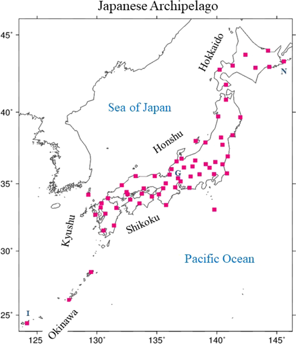
Geographical locations of the 63 stations used in this study over the Japanese archipelago and five region names (Hokkaido, Honshu, Shikoku, Kyushu, and Okinawa). Letters N, G, and I represent Nemuro, Gifu, and Ishigakijima stations, respectively.
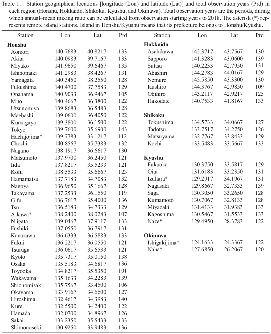
However, among dense AMeDAS, fully integrated surface observations of humidity, temperature, pressure, precipitation, wind, and other meteorological quantities have been made in limited stations. Approximately speaking, there are a few integrated observation stations in one prefecture. From these stations, those with an existing set of humidity, temperature and pressure records of longer than 120 years from the 1870s, 1880s or 1890s to 2018 were chosen. The starting dates (year and month) of these records differ widely depending on the stations. This selection results in a sparse distribution for the humidity dataset with roughly one station in one prefecture (subprefecture in Hokkaido) and mostly situated in the capital city (urban area) of each prefecture. There are some exceptions, i.e., two or three stations in one prefecture. Of these, a special case is observed, in which two stations, Hiroshima and Kure, are too closely located (about 18 km apart from each other) in the Hiroshima prefecture. Nevertheless, both data were used because there is no a priori reason to exclude one of them. In addition to the above mentioned stations, two and five stations beginning in the 1900s and the 1910s, respectively, were also included to fill the vacant regions of the station distribution in geographically important area such as remote islands in the sea.
In the surface observation data there are inevitably temporal inhomogeneities of abrupt changes due to instrument replacements for all the stations as well as the location movements for some stations, which relocated the observation fields within about 5 km from the original or previous positions. In addition, there are gradual changes due to the surrounding environment variations. For example, the effect of urbanization in big cities leads to rural–urban differences in humidity as well as temperature (Lee 1991). For instrument replacements, three instrument changes during humidity observation (Japan Meteorological Agency 2013) were noted as follows: Initial hair hygrograph; aspirated psychrometer observing dry–and wet–bulb temperatures (1950); lithium chloride hygrometer measuring dew point temperature (1971); electrical capacitive hygrometer (1996). The impact of instrument changes was assessed using a non–parametric test statistic (Lepage 1971), i.e., the Lepage test for the detection of discontinuity. First, a linear trend component was subtracted from the annual–mean data, and the test statistic was then evaluated, because the Lepage test includes the Wilcoxon rank–sum test (e.g., Lanzante 1996). The same sample length of 20 years in adjacent periods was adopted to diminish irrelevant interannual variations, since the sample length may affect the test result for shorter periods (Yonetani 1992a, b). The Lepage test indicates that the instrument changes did not introduce crucial impacts for the evaluation of long–term trend, similarly to Gaffen and Ross (1999).
The Lepage test was also made for the impacts of location moves for some stations. Aside from the much shorter time values such as instantaneous maximum or minimum temperature, results show that the location moves did not produce significant abrupt changes in annual and seasonal averages of the observed humidity and temperature values as in Gaffen and Ross (1999). This is because the spatial scale of atmospheric flow or air mass generally increases with the temporal scale, and vice versa. A variogram analysis (Hadano et al. 2004) demonstrates the annual–mean surface temperature of AMeDAS with some slight correction of altitude, latitude, and longitude to have a spatial representation of about 50 km, which is much larger than the station's movement distances. Following the results of the Lepage tests and the variogram analysis of AMeDAS data, an assumption was made that the seasonal– and annual–mean values are usable in the original form without any correction such as an adjustment for the discontinuous inhomogeneities (Karl and Williams 1987) for the trend analysis of surface humidity and temperature. However, there is one exception of Kobe station, which moved eastward by about 3.5 km from the middle (about 55 m altitude) of a hill to a seashore station (about 5 m altitude) nearly faced to wharves in 1999, leading to a substantial discontinuity in the observed record for the annual–mean absolute humidity. Thus, after excluding Kobe station, there remained 63 stations in total (Fig. 1, Table 1) for the long–term trends and variations analysis of surface humidity over the Japanese archipelago. The effect of urbanization was not treated in the analysis, though the dataset in highly–populated areas possibly included it surrounding the stations, which will be discussed in Section 6.
In the observation data prior to about 1960, there existed some limitations. First, available forms of humidity, pressure, and temperature were monthly–mean values in the shortest interval, and humidity was recorded as relative humidity. The errors stemming from the conversion from monthly–mean relative humidity to monthly–mean absolute humidity is investigated in the next section. Second, before about 1950, the available pressure was not station pressure but sea level pressure. Further, in two stations (Sapporo and Hakodate in Hokkaido) before around 1900, humidity and temperature observations exist but no record for sea level pressure was found. To substitute the recorded sea level pressure for that period, a climatological sea level pressure was employed for each month, which is an average for 30 years from the earliest years of pressure observation, because the effect of variations in atmospheric pressure on mixing ratio is very slight. For the conversion of sea level pressure to station pressure, the JMA formula (a hydrostatic balance equation) was used, which describes a relation between the two pressures with station temperature, station altitude, and climatological values of lapse rate and humidity over Japan.
The surface data prior to about 1990 was observed presumably at three–, four– or six–hour interval except for precipitation, and averaged/compiled in the form of monthly–mean. This process gives rise to uncertainty in the evaluation of monthly–mean mixing ratio evaluated from the monthly–mean temperature and relative humidity through the non–linear dependence of saturation vapor pressure on temperature. Initially, the accuracy and validity of the monthly–mean mixing ratio (rr_RH) calculated from the monthly–mean temperature, relative humidity, and station pressure were investigated through the comparison between rr_RH and monthly–mean mixing ratio (rr) based on a one–hour interval observation from 1990 to 2018. This comparison method is very similar to that used for monthly–mean dew point temperatures between one–hour and three–hour intervals data (Robinson 1998). Saturation vapor pressure was calculated through the formula of Tetens (1930), which is sufficiently accurate for most meteorological purpose except when extreme accuracy at low temperature is required (Murray 1967). Monthly–mean mixing ratios were calculated to the first decimal place similarly to the observed hourly data. Figure 2 shows the comparison between rr_RH and rr for annual means, and the relative errors (rr_RH - rr)/rr in 10 stations from the subarctic northernmost area through the temperate middle area to the subtropical southernmost islands area over the Japanese archipelago. Both the annual–mean mixing ratios agree very well for a wide range from about 5–17 g kg−1. The relative errors are generally within two percent, though they tend to be slightly larger for smaller mixing ratios, i.e., for lower temperatures because the denominator in the relative error decreases for smaller mixing ratios. Seasonally, the mixing ratio ranges from a minimum of about 2 g kg−1 in winter to a maximum value of about 22 g kg−1 in summer. The relative errors are mostly positive in summer but mostly negative in other seasons (not shown), resulting in much smaller relative errors in the annual means. This is because higher positive absolute errors in summer were substantially cancelled by smaller negative absolute errors in the other three seasons.
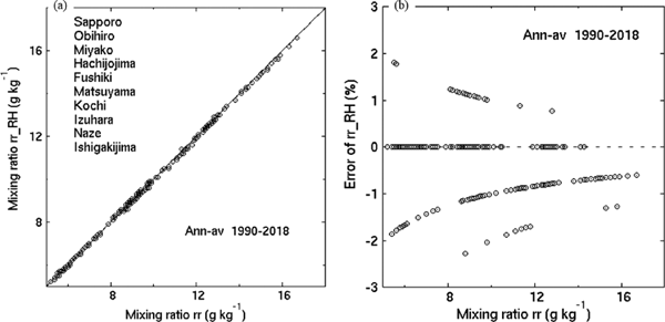
(a) Comparison of the annual–mean mixing ratios (g kg−1) between rr_RH and rr during 1990 and 2018 in 10 stations from the subarctic northernmost area through the temperate middle area to the subtropical southernmost remote islands area over the Japanese archipelago, and (b) the corresponding relative errors (rr_RH - rr)/rr (%). Station names are listed in the left upper place of (a).
Also in the trend evaluation the mixing ratio rr_RH is proved to have good accuracy, in which the trend analysis is made by the two methods described in the next section. The seasonal and annual trends of mixing ratio range from −1.0 g kg−1 to 5 g kg−1 century−1 for about 30 years from 1990 to 2018 (Fig. 3). The relative errors of rr_RH in the trend are mostly within 10 % (Fig. 3), indicating that rr_RH is accurate enough for the analysis of trend as a surrogate of rr. So far, the comparison is made using hourly data. Next, the effect of observation interval on rr_RH is evaluated. Before 1990, when automated observation instruments were introduced in the integrated observation stations, manual observation was made less frequently at three–hour or longer interval, depending on the observation periods. Thus, daily means nor monthly means were not calculated from the hourly data accordingly. Based on this, additional evaluations are made between the monthly–mean mixing ratios, rr_RH and rr, which are computed using longer time intervals, such as three and six hours for the same period from 1990 to 2018. It is found that rr_RH is also as accurate as that based on one–hour interval values (not shown). Comparisons made using longer hour intervals proved that rr_RH based on monthly–mean values can be quantitatively used for the evaluation of the long–term behavior of absolute humidity from the 1880s. As for the specific humidity, the monthly–mean specific humidity evaluated from the monthly–mean temperature, relative humidity, and station pressure and the monthly–mean specific humidity calculated from the one–hour data also exhibit slight differences between them, similarly to the mixing ratio. Henceforward, mixing ratio refers to rr_RH.
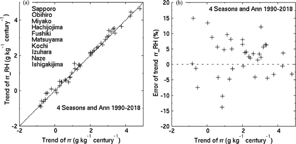
(a) Comparison of the annual–mean and four (spring, summer, autumn, and winter) seasonal–mean mixing ratio trends (g kg−1 century−1) between rr_RH and rr during 1990 and 2018 in 10 stations from the subarctic northernmost area through the temperate middle area to the subtropical southernmost remote islands area over the Japanese archipelago, and (b) the corresponding relative errors (%). Station names are listed in the left upper place of (a).
The linear trends in seasonal– and annual–mean mixing ratios were calculated by both the parametric least squares method and a non–parametric method, in the latter of which the slope and intercept of a regression line were calculated by Sen's slope estimator (Sen 1968) and the method by Siegel (1982), respectively. The linear trends in temperature and relative humidity were also evaluated by the same methods. Statistical significance of the trends was made using the Student's t–test for the least squares method and by the Mann–Kendall test for Sen's slope estimator. Seasonal means of spring (March, April, and May), summer (Jun, July, and August), autumn (September, October, and November), and winter (December, January, and February) were calculated if more than two months of data existed in each season. Otherwise, the seasonal mean was treated as a missing (non–valid) data. Similarly, the annual–mean was calculated as an average of four valid consecutive seasonal means, and thereby, the annual–mean of a year is an average from December of the previous year to November of the year concerned. Missing data were skipped and thus not used in the trend analysis. Sen's slope estimator is significantly more robust than the least squares method, because the former is insensitive to outliers. However, the two methods led to very similar results, and thereby only the results by Sen's slope estimator are shown henceforth.
Figures 4–6 show the time series of annual–mean temperature, relative humidity, and mixing ratio with regression lines from the 1880s or the 1890s to 2018 in Nemuro (northeastern Japan), Gifu (central Japan), and Ishigakijima (remote island in southwestern Japan) (see Fig. 1 for locations). Apparently these three stations' records do not exhibit significant jumps corresponding to the time of instrument changes around 1950, 1971, and 1996.
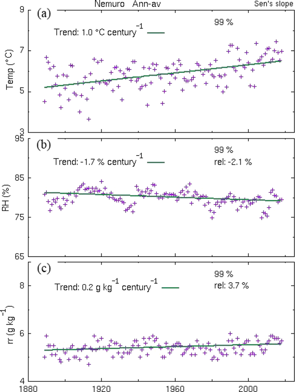
Time series of annual–mean and linear regression lines of (a) temperature (°C), (b) relative humidity (%), and (c) mixing ratio (g kg−1) in the northeastern Japan, Nemuro. Numbers in the left upper place are the linear trends (per century), and those in the in the right upper place represent the statistical significances and change rates in percentage.
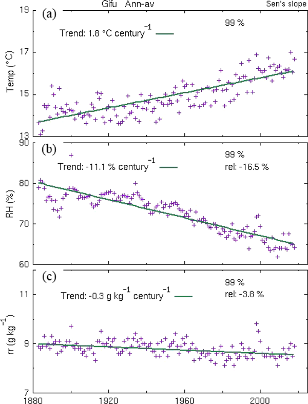
Time series of annual–mean and linear regression lines of (a) temperature (°C), (b) relative humidity (%), and (c) mixing ratio (g kg−1) in the central Japan, Gifu. Numbers in the left upper place are the linear trends (per century), and those in the in the right upper place represent the statistical significances and change rates in percentage.
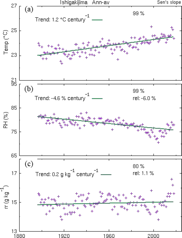
Time series of annual–mean and linear regression lines of (a) temperature (°C), (b) relative humidity (%), and (c) mixing ratio (g kg−1) in the southwestern Japan, Ishigakijima. Numbers in the left upper place are the linear trends (per century), and those in the in the right upper place represent the statistical significances and change rates in percentage.
The annual–mean temperature is commonly increasing at rates of 1.0, 1.8, and 1.2°C century−1 in the three stations with statistical significance of 99 %. On the other hand, the annual–mean mixing ratio exhibits a decrease of −0.3 g kg−1 century−1 in Gifu and an increase of +0.2 g kg−1 century−1 both in Nemuro and Ishigakijima. The relative trend of the mixing ratio calculated as a ratio of the (absolute) trend to the regressed value in the year 2000 is +3.7, −3.8, and +1.1 % century−1 in Nemuro, Gifu, and Ishigakijima, respectively. The magnitude of the relative trend remains approximately the same even if an average is used for the denominator, instead of the regressed value. One of the reasons why only Gifu exhibits a negative trend may stem from its geographical location. Nemuro and Ishigakijima stations are situated near the seashore, while Gifu is an inland station away (about 40 km) from the sea. However, as shown later, the geographical location does not play a crucial role because the locations of the stations having negative trend were systematically separated from those with positive trend irrespective of the distance from the sea.
In accordance with the warming (positive trends in temperature), relative humidity commonly exhibits a decreasing trend of −1.7, −11.1, and −4.6 % century−1 and relative change rates of −2.1, −16.5, and −6.0 % century−1 in Nemuro, Gifu, and Ishigakijima, respectively. In the three stations the quantitative relation Eq. (1c) among small changes in mixing ratio, relative humidity, and temperature approximately holds true. For example, the relative change of mixing ratio (∼ +4 %) for 100 years in Nemuro is nearly equal to the addition of the relative change of the relative humidity (∼ −2 %) and 7 % of the temperature change (+1°C). Among the three stations, Gifu exhibits the largest decrease in relative humidity by far because the decreasing trend in mixing ratio accelerates the decrease in relative humidity due to warming, while in Nemuro and Ishigakijima the increasing trend in mixing ratio decelerates it.
Figure 7 shows the spatial distribution of the annual–mean temperature trend over the Japanese archipelago from around the 1880s to 2018. All the stations show values of the same sign (positive) with most stations, exhibiting statistically significant warming of 1.0–2.5°C century−1, with nearly parallel features observed for each season (not shown). Similarly, the annual–mean relative humidity trend (Fig. 8) shows the same sign (negative) distribution except for one remote island station (Hachijyojima) and significantly decreasing values of −2 % to −12 % century−1 for most stations with small seasonality (not shown).
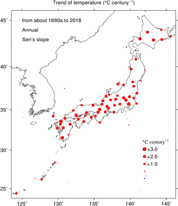
Spatial distribution of the annual–mean temperature trend (°C century−1) from about the 1880s to 2018. Red (blue) color represents positive (negative) value, and the area of circles is proportional to the values of trend. Triangles represent very small values, the magnitudes of which are less than 1.0.
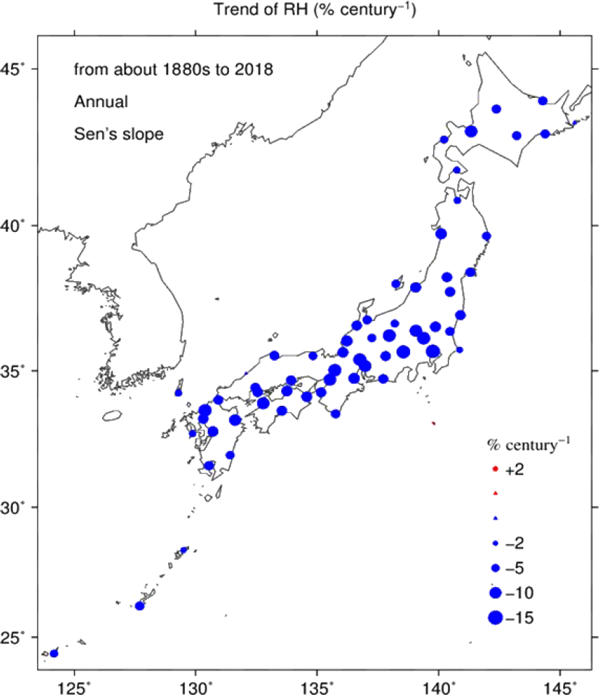
Spatial distribution of the relative humidity trend (% century−1) from about the 1880s to 2018. Red (blue) color represents positive (negative) value, and the area of circles is proportional to the values of trend. Triangles represent very small values, the magnitudes of which are less than 2.0.
On the other hand, the annual–mean mixing ratio trend (Fig. 9) displays different spatial distribution from the temperature or relative humidity trend. Three types of trends are observed: statistically significant increase (positive) and decrease (negative), and very slight changes of mixed sign (virtually zero). The negative trend stations of about −0.2 g kg−1 to −0.3 g kg−1 century−1, inclusive of slightly decreasing trend stations, are located approximately in the Pacific side of Honshu from the middle Tohoku (the northern Honshu) through Shikoku to the eastern Kyushu. It should be noted that the magnitude of negative trend scarcely correlates with population, i.e., a measure of urbanization. Significant positive trends of about 0.2–0.4 g kg−1 century−1 are observed over Hokkaido, Sea of Japan side of the western Japan, the western Kyushu, and the remote islands including Okinawa. The overall pattern of positive and negative trends distribution is similar for other seasons, and polarities of the trends are almost the same for all the seasons, except for most of the remote islands in winter.
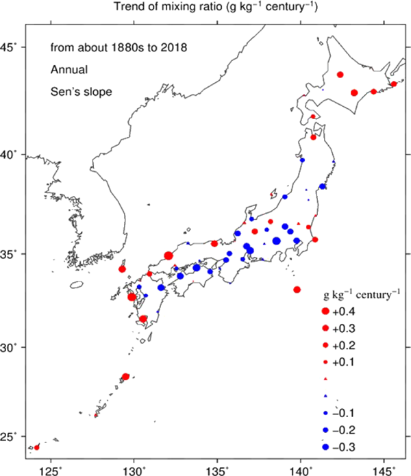
Spatial distribution of the annual–mean mixing ratio trend (g kg−1 century−1) from about the 1880s to 2018. Red (blue) color represents positive (negative) value, and the area of circles is proportional to the values of trend. Triangles represent very small values, the magnitudes of which are less than 0.1.
The magnitude of the trend in each station maximizes mostly in summer, minimizes in winter (Fig. 10), and takes intermediate values in spring and autumn. This seasonal variation in the mixing ratio trend approximately synchronizes with the seasonal cycle of mixing ratio and temperature, with usually increasing amplitude with latitudes over the Japanese archipelago. This is because the meridional gradient of temperature (and mixing ratio) is small in summer and large in winter and because the seasonal cycle is small in subtropics. The proportion of the summer climatological mixing ratio (maximum) to that of winter (minimum) is about five in subarctic Hokkaido, four in temperate Honshu, Shikoku, and Kyushu, and two in subtropical Okinawa. These figures are larger than the proportion of the summer trend to the winter trend in most stations as seen in Fig. 10. So that, the change ratio (the trend divided by the climatological seasonal mean) becomes similar or larger in winter than in summer, depending on the stations. However, the seasonality of the trend in the remote islands is very different. Here, the trend is significantly positive of about 0.3–0.5 g kg−1 century−1 during summer but weakly negative (∼ −0.2 g kg−1 century−1) or virtually zero during winter except for the Aikawa station in Sado island (Fig. 10). This is in contrast with the winter warming trend in the remote islands where the urbanization effect is supposed to be very small.
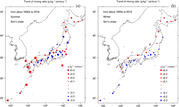
Spatial distribution of the seasonal–mean mixing ratio trend (g kg−1 century−1) from about the 1880s to 2018 for (a) summer and (b) winter. Red (blue) color represents positive (negative) value, and the area of circles is proportional to the values of trend. Triangles represent very small values, the magnitudes of which are less than 0.1.
An empirical orthogonal function (EOF) analysis was also made respectively for temperature, mixing ratio, and relative humidity data to investigate mutually independent (orthogonal) spatial patterns as to what extent the data variance is explained by each mode and to derive their temporal coefficients (scores). The EOF analysis is performed using the data from 1900 to 2018, because the starting years of observation differ widely from one station to another before 1900 as stated above. In addition, similar to the trend analysis, the data beginning in the 1900s and the 1910s were also included to cover a wider area in the sparse observation data. Prior to the EOF analysis, missing seasonal mean data were interpolated or extrapolated in the yearly time series of the same season. After, a moving average with a length of five years was applied for each seasonal–mean data to diminish short–term variations irrelevant to long–term components. The same procedure was made for the annual–mean data.
Figure 11 shows the first and the second EOF (EOF–1 and –2) scores and spatial patterns regressed to their scores for the annual–mean temperature. EOF–1 and –2 are found to explain 91 % and 3 % of the total variance, respectively. The EOF–1 spatial pattern is a distribution with similar signs and magnitudes and corresponds fairly well to the positive and almost uniform linear trend pattern of the annual–mean temperature shown in Fig. 7. In addition, the EOF–1 score displays nearly persistently increasing characteristics except during the 1960s and the 1970s, when there is substantially no tendency. This is similar to the annual surface temperature anomalies over the Japanese's 15 stations of weak urbanization (e.g., Japan Meteorological Agency 2019) and the global–mean land and sea surface temperatures (e.g., IPCC 2013). EOF–1 occupies a dominant (91 %) fraction of the total variance. Consequently, these facts (the persistent increase and dominant fraction of EOF–1) demonstrate that the annual–mean temperature linear trend is almost explained by the uniform persistent warming of EOF–1. Conversely, EOF–1 substantially consists of linear trend, which most likely stems from the greenhouse gas increase. On the other hand, the EOF–2 spatial pattern shows a seesaw–like distribution between the northern Japan and the southern Pacific area of the central and southwestern Japan. Its score is mostly comprised of decadal variations with a small contribution (3 %) to the total variance.
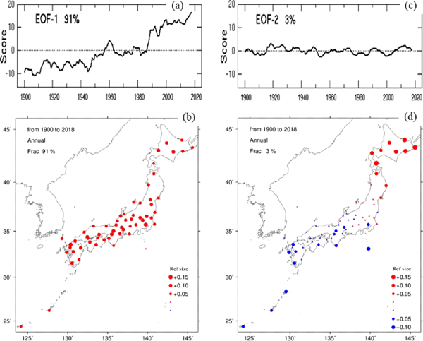
Annual–mean temperature EOF–1 (a) score and (b) spatial pattern (regressed to the score), and EOF–2 (c) score and (d) spatial pattern. Triangles represent very small values, the magnitudes of which are less than 0.05.
For the annual–mean mixing ratio, EOF–1, –2, and –3 (the third mode) scores are found to explain 49, 14, and 8 % of the total variance, respectively as shown in Fig. 12 along with their corresponding spatial patterns. The EOF–1 spatial pattern is comprised of similar magnitude values with the same sign, bearing close resemblance to that of the annual–mean temperature (Fig. 11). However, the EOF–1 score does not show any apparent trend until about 1960, after which it exhibits a prominent decreasing tendency for about 20 years during the 1960s and the 1970s. This term corresponds to the no–tendency period in the temperature EOF–1 score. After 1980, the EOF–1 score exhibits a clear increasing tendency with two bulges around 1990 and 2000.
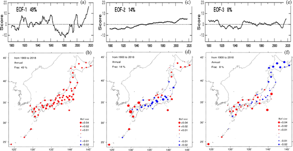
Annual–mean mixing ratio EOF score and spatial for (a)–(b) EOF–1, (c)–(d) EOF–2, and (e)–(f) EOF–3. Triangles represent very small values, the magnitudes of which are less than 0.01.
On the other hand, the EOF–2 spatial pattern is approximately composed of two areas of positive and negative values, which is very similar to the distribution of the annual–mean mixing ratio linear trend (Fig. 9). In addition, the EOF–2 score shows a nearly monotonically and significantly increasing trend throughout the whole period, indicating that the EOF–2 spatial pattern can be approximately interpreted as the linear trend pattern with drying and moistening areas, i.e., the significant decrease in the Pacific side of Honshu from the middle Tohoku through Shikoku to the east Kyushu and the significant increase in Hokkaido, Sea of Japan side of the western Japan, the west Kyushu, and Okinawa. In other words, EOF–2 is almost identical with the linear trend component in annual–mean mixing ratio. The EOF–3 spatial distribution represents a seesaw–pattern between the northern area (Hokkaido and Tohoku) and the western and southern Japan as the temperature EOF–2 spatial pattern (Fig. 11d).
For the annual–mean relative humidity, the EOF–1 and –2 scores and spatial patterns are exhibited in Fig. 13, wherein EOF–1 and –2 explain 76 % and 6 % of the total variance, respectively. The EOF–1 spatial pattern displays a distribution with the same sign and larger values from Kanto (Tokyo and its surrounding prefectures) through Chukyo (Nagoya and its surrounding prefectures) and Kansai (Osaka and its surrounding prefectures) to the northern Kyushu. Meanwhile, the EOF–1 score (Fig. 13a) shows almost persistent decreases except for a constant increase after the 2000s. If the sign is inverted, the EOF–1 spatial pattern (Fig. 13b) appears to be very similar to the linear trend distribution (Fig. 8), indicating that EOF–1 represents the linear trend component. The EOF–2 spatial pattern practically represents a seesaw–like distribution between the western Japan and the eastern Japan except for Hokkaido.
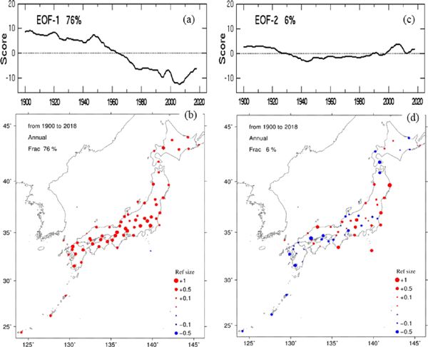
Annual–mean relative humidity EOF–1 (a) score and (b) spatial pattern, and EOF–2 (c) score and (d) spatial pattern. Triangles represent very small values, the magnitudes of which are less than 0.1.
Over the Japanese archipelago from about the 1880s to 2018 the linear trend in the annual–mean temperature exhibits the same polarity with positive sign in all the stations (Fig. 7). This is similarly observed with linear trend in the annual–mean relative humidity with negative sign except for a small positive value in Hachijyojima (Fig. 8). On the other hand, the linear trend in the annual–mean mixing ratio does not show the same polarity but is very approximately separated into three consecutive areas, depending on the signs (Fig. 9).: (1) negative area: Honshu, Shikoku, and eastern Kyushu, (2) positive area: Hokkaido, and (3) positive area: western Kyushu and Okinawa. Because these results reflect the climate change, the relation to the types of climate classification is first investigated. The spatial patterns in the annual–mean linear trends are found to be hardly correlated with the Köppen–Geiger climate classification (e.g., Beck et al. 2018) or other climate divisions (e.g., Koizumi and Kato 2012; Kusanagi 2016).
Next, the effect of sea surface temperature (SST) is examined. According to JMA analysis (e.g., Japan Meteorological Agency 2019) using the COBE-SST (Ishii et al. 2005), the annual–mean linear trends in SST surrounding the Japanese archipelago during the recent 100 years are 0.7–1.7°C century−1 with an area average of 1.1°C century−1 except for the marine area off northern Hokkaido. SST seasonal trends are also positive for all the seasons ranging from 0.5°C to 2°C century−1 (https://www.data.jma.go.jp/gmd/kaiyou/data/shindan/a_1/japan_warm/japan_warm.html). These facts indicate that the positive trends in SST alone cannot explain the reason why negative trends in the mixing ratio appear in Honshu, Shikoku, and the eastern Kyushu. This is because the warmer SST brings about positive changes in the near–surface mixing ratio over ocean. On the other hand, the spatial patterns in the mixing ratio linear trends are associated with changes in large– and synoptic–scale atmospheric circulation, which are probably caused by the global warming and with changes in micro–scale atmospheric circulation due to urbanization. However, this paper focuses on the analysis of surface data, and thus, investigation of the mechanisms responsible for these spatial patterns is a future work.
The linear trend from the 1880s or the 1890s to 2018 for the annual–mean mixing ratio ranges from about −0.3 g kg−1 to +0.4 g kg−1 century−1 (Fig. 9). Aside from the negative value area, the positive values of 0.2–0.4 g kg−1 century−1 over Hokkaido, Sea of Japan side of the western Japan, the western Kyushu, and the remote islands (Fig. 9) are much less than those in the continental and hemispheric scales for the absolute humidity data from the 1960s or the 1970s (e.g., Gaffen and Ross 1999; Dai 2006; Willett et al. 2008, 2010). The cause for this discrepancy may stem from not only geographical situations but also from the difference in the starting years of the analyses. Hence, using similar recent data from 1960, an additional trend analysis was carried out to investigate the trends in the recent years. Figure 14 displays the spatial distributions of the linear trends in the annual–mean temperature, relative humidity, and mixing ratio from 1960 to 2018. Comparison of these trends (Fig. 14) with those in the longer period (1880s–2018) (Figs. 7–9) reveals that the mixing ratio trend and the temperature trend in the recent period are very different from those in the longer period, while the relative humidity trend shows a small difference between the two periods. Quantitatively describing the causes of this conspicuous difference in the mixing ratio trends is currently very difficult because global warming and local urbanization effects are intricately involved with this as shown later.
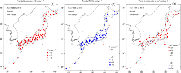
Annual–mean (a) temperature trend (°C century−1), (b) relative humidity trend (% century−1), and (c) mixing ratio trend (g kg−1 century−1) in the recent period from 1960 to 2018. Triangles represent very small values, the magnitudes of which are less than 1.0 in (a), 2 in (b), and 0.1 in (c).
To be specific, the mixing ratio trend in the recent period is significantly positive in most stations, being in stark contrast with clearly separated two areas of positive and negative values in the longer period of the 1880s–2018. In addition, the magnitudes of the positive trends over Hokkaido, Sea of Japan side of the western Japan, the western Kyushu, and the remote islands are approximately two times or more as large as those in the longer period. Figure 15 presents a quantitative comparison using scatter plots between the two periods for the linear trends in annual–mean temperature, relative humidity, and mixing ratio, together with the average trends during the two periods. The temperature trends in the recent period increase by 0.3°C to 1.3°C century−1 in most stations with an average change of about +1.1°C century−1 from 1.47°C to 2.52°C century−1.
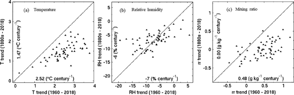
Comparison of the trends between the two periods, 1880s–2018 (ordinate) and 1960–2018 (abscissa), for annual–mean (a) temperature, (b) relative humidity, and (c) mixing ratio. Units are °C century−1 for the temperature trend, % century−1, for the relative humidity trend, and g kg−1 century−1 for the mixing ratio trend. Numbers in the graphs show the average values for the two periods.
Similarly, the mixing ratio trends rise by 0.2–0.8 g kg−1 century−1 in most stations with an average increase of about 0.5 g kg−1 century−1 from 0.0 to 0.5 g kg−1 century−1. At once, the ratio of the station numbers of negative trend to those of positive trend decreases from about 1/2 to as small as 1/6. This indicates that the increase in mixing ratio prevails over the Japanese archipelago during the recent period after the 1960s, being in coincident with that in continental or hemispheric extent for similar recent periods (e.g., Schönwiese et al. 1994; Gaffen and Ross 1999; Dai 2006; Willett et al. 2008, 2010). Quantitatively, this average increase of about 0.5 g kg−1 century−1 is also comparable with those in the continental or hemispheric scale (e.g., Gaffen and Ross 1999; Dai 2006; Willett et al. 2008, 2010).
On the other hand, the relative humidity trends extend their bounds from a range of 0 % to −15 % century−1 to a wider range (+5–−20 % century−1), while the average value changes about as small as −1 % century−1 from −6 % to −7 % century−1. These nearly the same negative averages of the relative humidity trends and Eq. (1) demonstrate that the dominance of drying (decrease in relative humidity) due to the warming over moistening (increase in relative humidity) due to the mixing ratio increase, as a whole, has been continuing since the 1880s over the Japanese archipelago.
Since the spatial distributions of the linear trends in annual–mean temperature, mixing ratio, and relative humidity over the recent period (Fig. 14) are very similar to their EOF–1 spatial patterns (Figs. 11–13), it is investigated whether there exist similar corresponding relations between the changes in the linear trends and those in the EOF–1 scores around 1960. The increased linear trend in the annual–mean temperature over the recent period agrees well with the steeper gradient of the EOF–1 score after the 1960s than before (Fig. 11a). Also for the annual–mean mixing ratio trend a similar close correlation holds true between the sharp increases in the linear trend and the EOF–1 score (Fig. 12a). These sharp increases qualitatively agree with the reference to the upper air absolute humidity by Ross and Elliott (2001) that most of the overall increase in the Northern Hemisphere's 850-hPa specific humidity probably occurred since 1973. This may indicate that the increased absolute humidity in recent years occurs not only at or near the surface but also in the lower troposphere up to 850 hPa in the Northern Hemisphere. It will be thus preferable to scrutinize not only precipitable water but also absolute humidity at each pressure level in the historical aerological data. On the other hand, the annual–mean relative humidity does not show substantial changes between the linear trends (Figs. 8, 14b) nor in the EOF–1 score (Fig. 13a) after the 1960s. This also indicates a good correspondence between them. These facts thereby demonstrate that the linear trend during the recent period after 1960 is also mostly explained by the EOF–1 in the longer period from 1900 for the annual–mean temperature, mixing ratio, and relative humidity.
The long–term trends and variations obtained in this study include the effects of climate forcings of various scales such as global greenhouse gas increase and local urbanization. The effect of variations in micro-environment surrounding the observation site is also included. In particular, the local urbanization effect on the temperature trend is substantially larger in Japan (Fujibe 2011) than that in China, Europe and North America, where its impact on the mean temperature trend is very small, in spite of definite warming in urban areas (Jones et al. 2008; Chrysanthou et al. 2014). Hence, the mixing ratio trend and the temperature trend should be discussed with consideration to urbanization because most integrated observation stations are located near the central urban area of capital city in each prefecture as stated before.
While it is well known that urbanization intensifies warming, i.e., urban heat island (UHI), less is known on how urbanization influences absolute humidity. Observation studies demonstrated that the loss of vegetation cover decreases the absolute humidity, i.e., urban dry island (UDI), through the reduction of evapotranspiration (Hao et al. 2015, 2018). The difference of surface latent heat flux between rural and urban areas is significantly positive in daytime, synchronizing with the diurnal cycle of solar radiation (Moriwaki et al. 2013). Thereby, absolute humidity difference is larger during daytime (Thapa Chhetri et al. 2017; Moriwaki et al. 2013) and summer season (Moriwaki et al. 2013) in the diurnal and seasonal cycles, respectively. The reduction of humid sea breeze penetration accompanying with urbanization (Fujibe 2009) is also involved with the mixing ratio decreasing trend, particularly in Japanese major islands (regions), where many stations are located within the sea breeze range (Fig. 1), depending on local geographical configuration.
On the other hand, mesoscale model simulations also proved that land cover and land use changes can induce UDI as well as UHI. By imposing land cover change due to an extensive urban growth from a present–day (ca. 1990) to a future year (ca. 2050) in the New York City metropolitan area, Civerolo et al. (2007) demonstrated that there occurs a substantial decrease in the surface mixing ratio and increase in the planetary boundary layer (PBL) height in the summer afternoon. A significant increase in surface temperature was also simulated with the areal extent of all of these changes generally coinciding with the area of increased urbanization. These indicate intensification of turbulent mixing in PBL stemming from destabilization due to enhanced heating at the surface. Since mixing ratio generally decreases with altitudes, turbulent mixing transports mixing ratio upward and thus decreases surface mixing ratio in PBL. Hence, the simulation of Civerolo et al. (2007) suggests that the increase in PBL height (intensification of turbulent mixing) is another factor for UDI.
The urbanization effect on the mixing ratio trend is much complicated, compared to that on the ubiquitously positive temperature trend, because both negative and positive values are analyzed for the mixing ratio trend (Fig. 9). Urbanization contributes partly to the mixing ratio negative trend in the Pacific side of Honshu from the middle Tohoku through Shikoku to the eastern Kyushu (Fig. 9). However, urbanization alone cannot explain why the magnitude of the negative trend hardly correlates with the population and why there are positive or virtually–zero values in big cities in northern, western, and southern regions such as Sapporo, Okayama, Hiroshima, Fukuoka, and Kagoshima. Concerning mixing ratio trends in big cities, the present result agrees with the JMA urbanization monitoring report (Japan Meteorological Agency 2013) that showed a significant decreasing trend in the annual–mean vapor pressure of −0.9 hPa to −0.6 hPa century−1 (mixing ratio trend of −0.6 g kg−1 to −0.4 g kg−1 century−1 for 1000 hPa station pressure) in Nagoya, Kyoto, and Tokyo for 1931–2012. These negative trends are in contrast to the small positive trends (0.3 hPa century−1 ∼ 0.2 g kg−1 century−1) in the other 15 cities which have undergone small urbanization. On the other hand, warming trends in big cities are significantly larger by 0.5°C to 1.7°C century−1 compared to an average of other 17 small urbanization cities (Japan Meteorological Agency 2013).
In addition to the positive or virtually–zero values in some big cities in the trend from about the 1880s, most stations exhibit significantly positive values in the mixing ratio trend during the recent period from 1960 (Figs. 14c, 15c), indicating that the contribution of UDI seemingly almost disappears after 1960, when the population in Tokyo Metropolis began to saturate and those in neighboring prefectures as well as other big cities began to rapidly increase (Fujibe 2011). Accordingly, not only urbanization but also other factors including global warming are thought to be intricately entangled in the mixing ratio trend. Be that as it may, the density of the long–record integrated observation stations (Fig. 1) is too sparse to isolate the local urbanization effect and hence to scrutinize each factor is beyond the scope of this paper.
Surface meteorological data archived by JMA from about the 1880s to 2018 over the Japanese archipelago are analyzed focusing on the long–term trends and variations in the water vapor mixing ratio, temperature, and relative humidity. Since those historical data prior to about 1960 is provided only in monthly–mean format, the validity of the monthly–mean water vapor mixing ratio calculated from monthly means of temperature, relative humidity, and surface pressure was investigated through the comparison with that based on one–hour interval data in recent years from 1990 to 2018. The comparison proved that the discrepancy between the two annual–mean mixing ratios is within two percent, and the difference in the linear trends is mostly less than ten percent.
The annual–mean temperature trends show positive values for all the stations with most stations exhibiting statistically significant warming of 1.0–2.5 °C century−1, and similar feature can be seen for each season. The annual–mean relative humidity trend also shows negative values and significantly decreasing of −2 % to −12 % century−1 for most stations with small seasonality. On the other hand, the annual–mean mixing ratio trend displays different spatial distribution from temperature or relative humidity trend. There are three types of trends: statistically significant increase (positive) and decrease (negative), and very slight changes of mixed sign. Significantly negative trends of about −0.2 g kg−1 to −0.3 g kg−1 century−1, are located approximately in the Pacific side of Honshu from the middle Tohoku through Shikoku to the eastern Kyushu. Significantly positive trends of about 0.2–0.4 g kg−1 century−1 are over Hokkaido, the western Japan along Sea of Japan, the western Kyushu, and the remote islands including Okinawa. The overall spatial pattern with positive and negative areas is similar for other seasons.
The EOF–1 spatial pattern of the annual–mean temperature is very similar to the linear trend pattern and its score displays nearly persistently increasing characteristics with a major (91 %) fraction of the total variance. Also, with inverted sign, the EOF–1 of annual–mean relative humidity has a similar spatial pattern to the linear trend distribution. Furthermore, its score decreases almost persistently with a major (76 %) contribution to the total variance. These facts indicate that the linear trends in the annual–mean temperature and relative humidity are almost explained by the nearly uniform persistent warming and drying of EOF–1 components and vice versa. On the other hand, for the annual–mean mixing ratio, EOF–2 (14 %) exhibits similar spatial pattern to the linear trend pattern and the EOF–2 score shows a nearly monotonically and significantly increasing trend throughout the whole period. This indicates that EOF–2 is almost identical with the linear trend in the annual–mean mixing ratio.
In recent years from 1960 the mixing ratio trend and the temperature trend are both significantly higher than those in the longer period from the 1880s, while the relative humidity trend remains nearly the same. The mixing ratio trend in the recent period is significantly positive in most stations and the magnitudes of the positive trends over Hokkaido, Sea of Japan side of the western Japan, the western Kyushu, and the remote islands are approximately two times or more as large as those in the longer period. The spatially averaged trends of about 0.5 g kg−1 century−1 for mixing ratio and of about +2.5°C century−1 for temperature are comparable with those in the continental or hemispheric scale for the similar recent periods in other studies.
The spatial distributions of the trends in the annual–mean temperature, mixing ratio, and relative humidity over the recent period from 1960 are found to be very similar to their EOF–1 spatial patterns for the longer period from 1900. In line with this, a close relation between the changes in the trends and those in their scores is observed around 1960. The increased linear trend in the annual–mean temperature for the recent period agrees well with the steeper gradient of the EOF–1 score after the 1960s than before. A similar close correlation holds true between the sharp increases in the linear trend and the EOF–1 score for annual–mean mixing ratio. On the other hand, the annual–mean relative humidity does not show substantial changes in the linear trend nor in the EOF–1 score around 1960, which also indicates a good correspondence between them.
Urbanization affects the long–term trends and variations in the surface humidity and temperature in many stations that are located in the central urban area in respective prefectures. However, urbanization effects on humidity are not as simply evaluated as its warming effect on the temperature over the Japanese archipelago. This is because the magnitude of negative trend scarcely correlates with population and because the negative trend area and positive trend area are distinctly separated, indicating other factors such as global warming also play crucial role on the surface humidity.