Abstract
Using data from the Sumatran GPS Array in Indonesia–a hero network in tectonic and earthquake studies–we study the summer intra-seasonal variability of precipitable water vapor (PWV) over Sumatra in years without strong inter-annual variability. Unlike most other studies that used external meteorological data to derive PWV from Global Positioning System (GPS) signal delays, we use the zenith wet delay (ZWD) time series estimated from a regular geodetic-quality processing routine as a proxy for PWV variations without using auxiliary meteorological data. We decompose the ZWD space-time field into modes of variability using rotated Empirical Orthogonal Function (EOF) analysis and investigate the mechanisms behind the two most important modes using linear regression analysis both with and without lags. We show that the summer intra-seasonal variability of daily ZWD over Sumatra in 2008, 2016, and 2017 was dominated by the South Asian Summer Monsoon and further influenced by dry-air intrusions associated with Rossby waves propagating in the Southern Hemisphere midlatitudes. Both active South Asian monsoons and dry-air intrusions contribute to the dryness over Sumatra during northern summer. Our results indicate an intra-seasonal connection between the South Asian and western North Pacific Summer Monsoons: when the South Asian monsoon is strong, it pumps atmospheric water vapor over the eastern Indian Ocean to feed into the western North Pacific monsoon. We also show a tropical-extratropical teleconnection where PWV over the southern Maritime Continent can be modulated by the activity of eastwardtraveling Rossby waves in the southern midlatitudes. Our case study demonstrates the use of regional continuously operating GPS (cGPS) networks for investigating atmospheric processes that govern intra-seasonal variability in atmospheric water vapor.
1. Introduction
The Global Positioning System (GPS) was originally designed for the purposes of positioning, navigation, and timing, yet it has emerged as a powerful tool for atmospheric water vapor sensing in ground-based GPS meteorology (Bevis et al. 1992). When GPS radio signals travel from satellites to ground receivers, they are refracted by the Earth's atmosphere, delaying their travel time. A significant portion of the delay is introduced by the permanent dipole moment of water vapor in the neutral atmosphere. This specific delay is referred to as the “wet delay” (Davis et al. 1985) or “tropospheric wet delay” as the troposphere contains nearly all atmospheric water vapor. The wet delay is determined primarily by the amount of water vapor integrated along the signal path (Askne and Nordius 1987), thus containing valuable information regarding the amount and distribution of atmospheric water vapor. The wet delay along any arbitrary path is typically modeled as zenith wet delay (ZWD), combined with mapping functions that account for the dependence of the satellite elevation angle (Niell 1996) and horizontal gradients that account for the azimuthal variability of the atmosphere (Davis et al. 1993). In order to achieve precise positioning that requires millimeter accuracy, ZWD must be estimated along with station coordinates and other geodetic parameters of interest. Thus, ZWD time series have long been produced as by-products of GPS position time series; however, such information is often disregarded by geodesists as noise.
Yet, a geodesist's noise is an atmospheric scientist's signal. Provided that there is ancillary pressure and temperature information, ZWD can be converted to an estimate of precipitable water vapor (PWV), that is, the height of liquid water if all atmospheric water vapor in a vertical column were condensed to liquid (Bevis et al. 1994). Although the basic concept of the GPS-PWV technique was introduced as early as 1992 (Bevis et al. 1992), its applications have continuously expanded since then owing to the exponential growth of national, regional, and local networks of continuously operating GPS (cGPS) stations over the past few decades. Published GPS-PWV studies have mostly focused on developing and refining the technique itself, comparing it with other techniques, calibrating other instruments, and improving numerical weather prediction and reanalysis models through validation or assimilation (Guerova et al. 2016). More recently, GPS-PWV has been applied in climate studies largely to two extreme ends of the broad time scale that GPS observes: either long-term trends (e.g., Nilsson and Elgered 2008; Wang et al. 2016) or diurnal and subdiurnal cycles (e.g., Dai et al. 2002; Pramualsakdikul et al. 2007). The intra-seasonal variability of GPS-PWV has been tackled only in a few studies, either being analyzed among a broad range of temporal scales or used to support results from other PWV datasets (Bock et al. 2007, 2008; Poan et al. 2013). Such a bimodal distribution of GPS-PWV studies in time scale is not surprising as the most important advantages of the GPS-PWV technique, in comparison to other PWV-sensing techniques such as radiosondes and satellite-borne sensors, are high temporal resolution and long-term stability. However, in order to fully exploit the continuous records of high-resolution GPS-PWV data over long periods of time, the understanding and isolation of the intermediate-frequency signals such as intra-seasonal variability contained therein are also essential.
Therefore, in this study, we present an approach of analyzing ZWD data from a regional cGPS network–the Sumatran GPS Array (SuGAr)–to demonstrate that such network, with the help of reanalysis datasets, can be useful for investigating the intra-seasonal variability of PWV as well as its driving mechanisms. We use the ZWD time series that are by-products of a regular geodetic-quality processing routine as a proxy for PWV variations so that auxiliary meteorological data are not required to derive PWV from ZWD. Our approach is particularly cost-effective if applied to the large number of existing cGPS networks that were not originally established for atmospheric purposes (Blewitt et al. 2018).
The SuGAr was initially established in 2002 for tectonic and earthquake studies, and thus, it has been well known and mostly used for studying deformations related to a series of recent great earthquakes along the Sumatran subduction zone (e.g., Feng et al. 2015). The network spans latitudinally from 5°N to 6°S, straddling the equator, with the majority of the GPS stations located on the Sumatran forearc islands and the west coast of Sumatra (Fig. 1). Coincidentally, Sumatra and its forearc islands lie along the western periphery of the Maritime Continent (Ramage 1968)–the “boiler box” of the atmosphere that produces the world's largest regional rainfall (e.g., Qian 2008; Yamanaka 2016; Yamanaka et al. 2018). Although the uneven spatial distribution of the SuGAr might not be optimal for atmospheric observations, the longitudinal location, long latitudinal span, and minute-scale high temporal resolution collectively make the SuGAr a valuable and cost-effective moisture-sensing network for investigating multiscale atmosphere processes that affect the western Maritime Continent. Thus far, the SuGAr and other GPS stations in Sumatra and its forearc islands have been mainly used to study diurnal cycles (Wu et al. 2003, 2008; Fujita et al. 2011; Torri et al. 2019). To the best of our knowledge, no one has yet used these stations to study intra-seasonal variability. Both global and regional lack of GPS-PWV intra-seasonal studies motivate us to focus on intra-seasonal variability in this paper.
The climate over Sumatra exhibits seasonal variations due to the Asian-Australian monsoon (e.g., Chang et al. 2005). Monsoonal rainfall over southern Sumatra peaks during the Australian summer monsoon season (December to March), whereas northern Sumatra experiences a double-peak rainfall seasonality in northern fall (October to November) and northern spring (March to May) (e.g., Hamada et al. 2002; Aldrian and Susanto 2003). Despite differing annual peaks, both northern and southern Sumatra experience a concurrent dry season when the Asian summer monsoon dominates during northern summer (June to September) (e.g., Hamada et al. 2002; Aldrian and Susanto 2003). Here, we focus on the intraseasonal variability of this dry season over Sumatra as droughts tend to occur in this dry season, leading to adverse socio-economic consequences such as water shortages, crop reduction, and increased risk of fires and transboundary haze. However, because intraseasonal variability over Sumatra can be modulated by inter-annual variability driven predominantly by the El Niño-Southern Oscillation (ENSO) (e.g., Hendon 2003) and Indian Ocean Dipole (IOD) (Saji et al. 1999), we choose for our case study 2008, when the dry season was not strongly influenced by either the ENSO or IOD.
In the rest of the paper, we first document the details of our methods, including GPS processing, ZWD estimation, PWV derivation and comparison, rotated EOF analysis, and linear regression analysis in Section 2. We then present and discuss our results for the 2008 northern summer in Sections 3 and 4. In Section 3, we show that the first mode of the intra-seasonal ZWD variability is driven by the South Asian Summer Monsoon, confirming that active South Asian monsoon spells lead to dry conditions over Sumatra. In Section 4, we show that the second mode is caused by extratropical dry-air intrusions associated with eastward-traveling extratropical Rossby waves, providing the first in-situ evidence for extratropical dry-air intrusions reaching equatorial latitudes within 5° south of the equator over the Maritime Continent. In Section 5, we present our additional results for the 2016 and 2017 northern summers, which support our main conclusions for 2008.
2. Methods
2.1 GPS data and processing for estimating ZWD
We processed the daily GPS Receiver Independent Exchange Format (RINEX) files using the GPS-Inferred Positioning System and Orbit Analysis Simulation Software (GIPSY-OASIS) version 6.2 developed at the Jet Propulsion Laboratory (JPL) (Zumberge et al. 1997). GIPSY implements the precise point positioning approach in which the carrier phase and pseudorange data from a single receiver are used to estimate the parameters specific for this receiver, while satellite orbit and clock parameters are held fixed at their values determined in a global solution. We used the JPL final precise satellite orbit and clock products, which are routinely generated by the JPL as part of their International GNSS Service (IGS) global network analysis. GIPSY uses undifferenced data so that absolute ZWD values can be obtained for individual stations.
As the full details of the GPS processing strategy have been provided in Feng et al. (2015), here we outline and highlight only the procedures central to the ZWD estimation, which are essentially described by Eq. (1) (Bar-Sever et al. 1998)
where STD is the slant total delay in the neutral atmosphere, ZHD is the zenith hydrostatic delay,
e is the elevation angle measured from the local horizon to the line of sight,
Mh (
e) and
Mw (
e) are hydrostatic and wet mapping functions,
Gn and
Ge are north and east tropospheric horizontal gradients, and
γ is the azimuth angle measured clockwise from the north.
GIPSY uses a model that does not require any surface meteorological data to calculate an a priori ZHD. We held this nominal ZHD fixed during processing while estimating the time-varying ZWD as a stochastic random-walk process with a sigma of 5 × 10⁻⁸ km s−1/2 (= 3 mm h−1/2) using a Kalman filter technique (Tralli and Lichten 1990). To account for the azimuthal variability of the atmosphere, we estimated tropospheric horizontal gradients as random-walk parameters with their sigma as 5 × 10⁻⁹ km s−1/2 (= 0.3 mm h−1/2) (Bar-Sever et al. 1998). To minimize the effects of multipath and atmospheric propagation errors at low elevation angles, we used the updated Vienna mapping functions in a grid file database (VMF1GRID) (Boehm et al. 2006) to relate ZHD, ZWD, and horizontal gradients in the zenith direction to slant delays at elevation angles down to 7° (Bar-Sever et al. 1998).
We estimated the time-varying ZWD every 5 min or 10 min depending on whether the GPS data were collected at a sampling rate of 15 s or 2 min. Therefore, the resulting ZWD time series have a temporal resolution of either 5 min or 10 min. With focus on intra-seasonal variabilities that have a period longer than one day, we calculated daily averages and removed the time-mean for all ZWD time series. We disregarded stations that had > 20 % missing data. For stations that missed a small number of values at discrete times, we filled their gaps using linear interpolation.
2.2 ZWD as a proxy for PWV
As the utility of ground-based GPS stations for PWV studies is partially hampered by the need for auxiliary meteorological data to convert from ZWD to PWV, many efforts have been spent on developing optimal methods of incorporating meteorological data to derive more accurate PWV (e.g., Wang et al. 2007). As opposed to these efforts, we use ZWD directly for our analysis because our objective is to investigate the variability (not absolute value) of PWV. We show in this section that the GIPSY-estimated ZWD time series for SuGAr stations on a daily time scale are linearly related to the PWV time series converted from ZWD using more sophisticated approaches that incorporate auxiliary meteorological data.
ZWD typically accounts for ∼ 10 % of the zenith total delay in the neutral atmosphere, so the accurate estimation of ZWD requires the precise determination of the remaining delay–ZHD, which is caused by the induced dipole moments of dry gases and water vapor (Davis et al. 1985). ZHD can be accurately inferred from surface air pressure (Ps) measured using well-calibrated barometers (Hopeld 1971), but pressure gauges collocated with GPS stations are rare. In most cases, Ps has to be interpolated from nearby meteorological measurements or model calculations with lower, albeit adequate, accuracy. In practice, most GPS processing packages simply utilize empirical models without Ps measurements to calculate an a priori ZHD so that ZWD is estimated as a correction to this nominal value.
For the case of GIPSY, the a priori ZHD was computed using Eq. (2) (Tralli et al. 1988)
where ZHD [m] is a linear function of surface atmospheric pressure
Ps [bar] and
Ps is approximated as an exponential function of station height
h [m]. Because 1.013 bars is sea level pressure,
h ideally should be the height above mean sea level or the geoid, but in practice, the height above the GRS80 ellipsoid is adopted for
h. The GIPSY ZHD equation requires no surface pressure data and assumes the same gravity (thus the same linear slope) everywhere, so it is easy to implement and is well suited for precise positioning, but meanwhile, such simplification inevitably sacrifices some degree of accuracy. Any error in the a priori ZHD is absorbed into ZWD estimations.
In order to assess the impact of the a priori ZHD value, we calculated daily ZHD time series for our study period using the more involved Saastamoinen model (Saastamoinen 1972) that accounts for the slight variation in gravity with station latitude φ [degree] and height h [m]
Because no pressure measurements were made at the SuGAr stations, we obtained daily averaged
Ps for each station using the nearest grid point from the National Centers for Environmental Prediction (NCEP) Climate Forecast System Reanalysis (CFSR) 6-hourly 0.5° × 0.5° reanalysis products (
Saha et al. 2010) and the European Centre for Medium-Range Weather Forecasts (ECMWF) ERA-Interim 6-hourly 0.5° × 0.5° reanalysis products (
Dee et al. 2011). The differences between the GIPSY a priori ZHD value and CFSR or ERA-Interim ZHD time series were then used to correct the GIPSY ZWD estimations to obtain the CFSR-corrected or ERA-Interim-corrected ZWD time series.
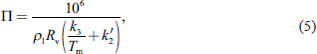
ZWD can be converted to PWV via a dimensionless conversion factor Π (Bevis et al. 1994)
where PWV and ZWD are in the same unit of length and Π is given by
Askne and Nordius (1987)
where
ρl (= 1000 kg m
−3) is the density of liquid water,
Rv (= 461.5 J kg
−1 K
−1) is the specific gas constant for water vapor,
k3 (= 3739 ± 12 K
2 Pa
−1) and
k′2 (= 0.221 ± 0.022 K Pa
−1) are the refractivity constants (
Bevis et al. 1994), and
Tm is the water-vapor-weighted mean temperature of the atmosphere, which is defined based on the mean value theorem in
Davis et al. (1985) as
where
h is the station height,
pv is the partial pressure of water vapor, and
T [K] is the absolute temperature.
With the values of ρl, Rv, k3, and k′2 given as constants, Tm becomes the only changing parameter that affects the value of Π. We calculated daily Tm for each station through direct integration of Eq. (6) using the daily averaged humidity and temperature profiles of the nearest grid point obtained from the same CFSR and ERA-Interim products that were used for obtaining Ps. We made no adjustments to correct the distance or height difference between GPS stations and their corresponding grid points. We then combined the CFSR-derived or ERA-Interim-derived Tm time series with the CFSR-corrected or ERA-Interim-corrected ZWD time series that were obtained earlier to compute the corresponding PWV time series.
As Π values for tropical stations stay almost constant throughout all years (Manandhar et al. 2017), we also multiplied the GIPSY ZWD estimations by a constant Π of 0.163 to derive PWV directly without any additional corrections. These GIPSY-derived PWV time series show the same variations as the CFSR-corrected and ERA-Interim-corrected PWV time series, despite their differences in magnitude (Fig. 2). The correlations of the GIPSY-estimated ZWD time series with either the CFSR-corrected or ERA-Interim-corrected PWV time series are > 0.99 for all our stations, suggesting that the ZWD that we estimated with GIPSY can be directly used as a proxy for PWV.
2.3 Comparisons of PWV with other datasets
Besides the ground-based GPS approach, many other techniques have been developed to determine PWV, either in situ using balloon-borne radiosondes or remotely from both ground and space using various types of passive or active sensors (e.g., Kämpfer 2013; Wulfmeyer et al. 2015). In order to validate our GIPSY-derived PWV time series, we compared them with daily PWV from two other datasets that are available. The first dataset is the Moderate Resolution Imaging Spectroradiometer (MODIS) Level-3 Atmosphere Daily 1° × 1° Global Gridded Product Collection 6.1 for Terra and Aqua satellites (King et al. 2003). We averaged the Terra-MODIS and Aqua-MODIS PWV thermal infrared retrievals at grid points closest to the SuGAr stations to obtain the MODIS-derived PWV for comparison. The second dataset is the Remote Sensing Systems (RSS) Version 7 daily 0.25° × 0.25° binary products retrieved from a series of satellite passive microwave radiometers using a unified, physically based algorithm (Wentz 1997, 2013). We used the products of three radiometers that were in orbit during our study period in 2008, including the Special Sensor Microwave Imager (SSM/I) onboard the United States Air Force Defense Meteorological Satellite Program (DMSP) satellite F13, and the Special Sensor Microwave Imager Sounder (SSMIS) onboard DMSP satellites F16 and F17. We averaged the F13-SSM/I, F16-SSMIS, and F17-SSMIS PWV microwave retrievals at grid points closest to the SuGAr stations to obtain the RSS-derived PWV for comparison.
Although thermal infrared retrievals are affected by the presence of clouds (e.g., Susskind et al. 2003), passive microwave retrievals work under almost all weather conditions, except for heavy precipitation, but their accuracy is high only over ice-free oceans and degrades appreciably over land because of larger and more variable surface emissivities (e.g., Mears et al. 2015). By contrast, ground-based GPS is a 24-h all-weather system because GPS satellites transmit L-band microwave signals that pass through the atmosphere without much signal attenuation (Spilker 1996). Therefore, land-based GPS networks complement perfectly satellite-borne passive microwave sensors that perform well only over the oceans.
Our GIPSY-derived PWV time series show general agreement in large-amplitude variations with both the MODIS-derived and RSS-derived PWV; however, they have differences in small fluctuations (Fig. 3). Because clouds are the norm in the tropics, the MODIS thermal infrared technique missed more days than the two microwave-based techniques, except for an inland SuGAr station JMBI (Fig. 1) where the RSS-derived PWV had more data gaps than the MODIS-derived PWV (Fig. 3). The RSS grid points used for JMBI were located east of Sumatra in a sea area partially surrounded by islands. The land contamination degraded the accuracy of the RSS retrieval algorithm (Mears et al. 2015), likely causing the many missing data of the RSS-derived PWV for JMBI. The MODIS thermal infrared retrievals seem to overestimate high values compared to the GIPSY-derived PWV (Fig. S1), whereas the RSS-derived retrievals show no clear bias relative to the GIPSY-derived PWV (Fig. S2). For all stations, the GIPSY-derived PWV is more consistent with the RSS-derived PWV than the MODIS-derived PWV (Figs. 3, S1, S2), suggesting that the two microwave-based techniques are relatively consistent in coastal areas. The overall agreement between GPS-PWV and microwave PWV retrievals has also been shown for small islands in the open ocean (Mears et al. 2015). Note that the absolute values of our GIPSY-derived PWV may contain biases as we did not apply any height and distance adjustments, and MODIS-derived and RSS-derived PWV may also have their own biases (e.g., Prasad and Singh 2009; Mears et al. 2015). A careful comparison of PWV datasets over Sumatra is a subject of a future paper.

We used EOF analysis, also known as Principal Component Analysis, to decompose the ZWD space-time field into a set of mutually orthogonal spatial patterns along with their associated mutually uncorrelated temporal variations. Although the spatial patterns and temporal variations have many alternative names in various literatures, we refer to them as EOFs and Expansion Coefficients (ECs), respectively. The elements of EOFs are called loadings that represent the covariances between each GPS station and each EOF (Richman 1986), whereas the elements of ECs indicate the strength of the corresponding EOF on a given day. Because of the orthogonality condition of EOFs, each pair of EOF and EC is regarded as a mode of variability that explains a fraction of the total variance in the ZWD field. We sorted the modes in descending order of their contribution so that the lower the mode is the more variance it explains. We find that the first two modes explain 66 % and 19 % of the total variance, respectively, totaling 85 %, in contrast with 6 % explained by the third mode, so we focus on interpreting only the first two modes (Fig. 4). We further rotated the EOFs using the Varimax criterion (Kaiser 1958), which finds a new orthonormal basis that maximizes the spread of the variances along the axes of the basis to achieve a simple structure (Richman 1986). The resulting rotated EOFs (REOFs) remain orthogonal, but the corresponding rotated ECs (RECs) have nonzero correlation. Note that flipping the signs of both EOF and EC for a mode results in an alternative expression of the mode that also satisfies the EOF solution. To be consistent with common sense, we used the expression in which positive/negative (+/−) loadings represent wetter/drier conditions.

EOF1 is one sign (−) across the whole network, while EOF2 depicts a network-wide northwest-southeast (+ −) dipole pattern (Figs. 5a, b). In comparison to the network-wide patterns obtained from the EOF analysis, the rotated EOF analysis yields more localized patterns with REOF1 and REOF2 influencing primarily the northern and southern stations, respectively (Fig. 5). REC1 (Fig. 6a) and REC2 (Fig. 6b) also seem to separately capture the temporal evolution of ZWD at the northern and southern stations (Fig. S3). Localized patterns are often more physically meaningful than network-wide patterns (e.g., Hannachi et al. 2007). Thus, the rotated EOF results are used in the rest of the paper for the physical interpretation of ZWD variability, which, in turn, justifies the necessity of rotation for our case.
2.5 Linear regression analysis
The rotated EOF analysis is a purely mathematical method without a physical basis; therefore, it does not provide direct insight into the physical processes that drive ZWD variability. In order to gain more insight, we applied linear regression analysis both with and without lags to investigate the relationships of our obtained RECs with various atmospheric quantities in the NCEP CFSR 6-hourly 0.5° × 0.5° products (Saha et al. 2010).
We first calculated daily averages for each quantity of interest at each grid point within a domain of interest, which is either a much wider region than the SuGAr network at a certain depth or a vertical profile. We then constructed the linear regression between the time series of a physical quantity Y(t) and REC1 or REC2 at any grid point i in the domain as follows:
where
ai is the regression constant and
bi is the regression coefficient. We performed this linear regression for all grid points within the domain, but we only retained the results for those with sufficiently low
p-values (< 0.05) as only low
p-values indicate the statistically significant correlation of
Y(
t) with REC. If statistically significant linear correlations are found between a REC and physical quantity at many locations within the domain, we plotted values of
bi as regression maps or profiles to show the pattern of anomalies in
Y associated with a standard REOF event that has a unit strength (REC = 1).
3. The first mode REOF1: Monsoon variations
The obvious candidate responsible for the first mode is the monsoon. The Asian-Australian monsoon system has been traditionally divided into four interlinked subsystems, including the East Asian monsoon, South Asian monsoon, western North Pacific monsoon, and Australian monsoon (Wang and LinHo 2002; Yim et al. 2014). The last three monsoon subsystems intersect at Sumatra, and the ZWD variability over Sumatra is thus more likely influenced by those three subsystems.
To quantify the large-scale variability of the South Asian monsoon, western North Pacific monsoon, and Australian monsoon, we constructed monsoon circulation indices that measure low-level monsoon trough vorticity in a unified approach (Yim et al. 2014). This approach uses the difference of 850-hPa zonal winds (U850) averaged over a domain equatorward and another domain polarward of the monsoon trough to express a north-south gradient of low-level zonal winds. We adopted U850 (5–15°N, 40–80°E) minus U850 (20–30°N, 70–90°E) as the South Asian monsoon index (Wang et al. 2001), U850 (5–15°N, 100–130°E) minus U850 (20–35°N, 110–140°E) as the western North Pacific monsoon index (Yim et al. 2014), and U850 (0–15°S, 90–130°E) minus U850 (20–30°S, 100–140°E) as the Australian monsoon index (Yim et al. 2014). We obtained the zonal winds from the NCEP CFSR 6-hourly 0.5° × 0.5° products to compute the three regional monsoon indices.
To determine which subsystem best explains the first mode, we smoothed REC1 and the three monsoon indices with a 5-day running mean, and calculated Pearson product-moment correlation coefficients between REC1 and the indices for lags ranging from −30 days to 30 days. We obtain the highest correlation coefficient of 0.75 when the South Asian monsoon index leads REC1 by three days (red curve in Fig. 6e). Slightly lower peak correlations of 0.53 and −0.64 are achieved when REC1 leads the western North Pacific monsoon index by 3 and 19 days, respectively (blue curve in Fig. 6e). The lowest peak correlations are found between the Australian monsoon index and REC1, with their lead-lag correlations without strong peaks (gray curve in Fig. 6e), showing an expected weaker association between the Australian monsoon, inactive during northern summer, and REC1. By contrast, high peak correlations of REC1 with the South Asian monsoon index and western North Pacific monsoon index suggest a strong association between the first mode and the Asian summer monsoon (Fig. 6f), though not necessarily implying immediate cause and effect relations. We thus conducted linear regression analysis for REC1 derived from our ZWD data with the PWV, specific humidity, and winds taken from the CFSR to further investigate the relationships between REC1 and the South Asian Summer Monsoon and western North Pacific Summer Monsoon.
The resulting PWV regression map shows that Sumatra and its forearc islands experience drier-than-usual conditions during a standard REOF1 event (Fig. 7a), consistent with the network-wide negative loadings of REOF1 (Fig. 5c). Centered over Sumatra, the dry anomaly extends westward to 80°E in the equatorial Indian Ocean and eastward to western Borneo (Fig. 7a). Vertically, as shown by the specific humidity regression profiles that cut through the center of the dry anomaly, it is mostly concentrated within the middle troposphere between 750 hPa and 450 hPa, not penetrating down to the atmospheric boundary layer (Figs. 7b, c). This equatorial dry anomaly is coupled with a wet anomaly located in the northern part of the Arabian Sea, Indian subcontinent, and Bay of Bengal (Fig. 7a). The coupled wet-dry anomalies closely resemble previously identified key features of composite outgoing longwave radiation (OLR) anomalies obtained for active spells of the South Asian Summer Monsoon (Rajeevan et al. 2010; Pai et al. 2016)–OLR is often taken as a proxy for deep convection and the associated rainfall because deep convective clouds have cold tops that emit low OLR. Specifically, the wet anomaly coincides approximately with negative OLR (positive rainfall) anomalies along the South Asian Summer Monsoon trough, whereas the dry anomaly overlaps a large portion of positive OLR (negative rainfall) anomalies that extend along the equator roughly from 60°E in the Indian Ocean to 140°E in the western Pacific (Rajeevan et al. 2010; Pai et al. 2016). The close resemblance of the coupled wet-dry anomalies to the composite OLR anomalies of active spells leads us to suggest that these anomalies are a feature associated with an active South Asian Summer Monsoon. When the South Asian Summer Monsoon is strong, abundant moisture converges into its action center, producing intense convection, and at the same time, dry conditions are brought to Sumatra, suppressing convection. A reverse pattern in which the South Asian Summer Monsoon convective region and Sumatra experience dry and wet conditions, respectively, dominates monsoon breaks, as suggested by the OLR break composites (Rajeevan et al. 2010; Pai et al. 2016). Thus, during northern summer, the moisture conditions over Sumatra are always opposite to those over the South Asian Summer Monsoon convection center. This locked inverse relationship explains why the lead-lag correlations between REC1 and the South Asian monsoon index have only one single strong peak (red curve in Fig. 6e). Because the leadlag correlations between REC1 and the western North Pacific monsoon index show two strong peaks instead of one (blue curve in Fig. 6e), we speculate that the western North Pacific Summer Monsoon convective region and Sumatra do not always behave oppositely. Unfortunately, no similar composite studies have been conducted for active spells and breaks of the western North Pacific Summer Monsoon to corroborate our speculation.

Geographically between the dry and wet anomalies, a narrow belt of high-speed wind anomalies at 850 hPa blows eastward from the Arabian Sea via peninsular India to the Bay of Bengal (Fig. 8e). This belt of fast-moving westerlies is part of a strong cross-equatorial low-level jet stream (LLJ) (Findlater 1969a, b) that attains its maximum speed of 10–25 m s−1 at 850–925 hPa (Wilson et al. 2019). Developing only during the months of the South Asian Summer Monsoon (Joseph et al. 2006), the LLJ picks up a large amount of moisture over the Indian Ocean from both hemispheres to feed the monsoon rainfall over South Asia (Saha 1970; Cadet and Reverdin 1981). The maximum winds of the LLJ lie along different latitudes at different phases of the South Asian Summer Monsoon: during monsoon onset, they flow east between the equator and peninsular India; during active monsoon periods, they pass through peninsular India near 15°N; and during monsoon breaks, they split into two branches, with one blowing south of peninsular India near 5°N and the other through north India near 25°N (Joseph and Sijikumar 2004). The fact that the belt of high-speed wind anomalies enters peninsular India between 10°N and 20°N (Fig. 8e) strongly suggests the wind anomalies to be another manifestation of an active South Asian Summer Monsoon.
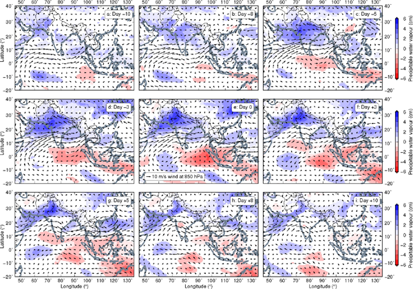
The coupled wet-dry anomalies and in-between belt of high-speed wind anomalies, together with our derivation that the highest correlation is obtained when lagging REC1 behind the South Asian monsoon index by three days, lead us to conclude that the first mode is driven by the South Asian Summer Monsoon with a delay response of a few days. To examine how the wet, dry, and wind anomalies evolve during the life cycle of one standard REOF1 event, we additionally lagged REC1 by −10 to 10 days for lead-lag linear regression analysis with the CFSR PWV and winds at 850 hPa (Fig. 8) and 600 hPa (Fig. 9). Note that we use the wet anomaly as an indicator of the convective activity of the South Asian Summer Monsoon.

On day −8, the wet anomaly emerges before other anomalies appear (Fig. 8b), suggesting that the convective heating of the South Asian Summer Monsoon is the main engine that drives other processes. As the wet anomaly grows bigger and stronger, the LLJ intensifies, with its core shifting northward from the south of peninsular India to over peninsular India within the next 2–3 days (Fig. 8c). A similar lag of 2–3 days has been found between the convection over the Bay of Bengal and 850-hPa zonal winds over both the Arabian Sea (Srinivasan and Nanjundiah 2002) and peninsular India (Joseph and Sijikumar 2004), with more intense convection leading to stronger westerlies. The intensification of the LLJ can be understood as a transient response to the sudden switch-on of an off-equatorial heat source (Heckley and Gill 1984), which is, in this case, the increased convective activity over the wet anomaly. The intensified LLJ, in turn, enhances the advection of moisture into the Indian subcontinent and increases the cyclonic vorticity and consequent low-level moisture convergence north of the LLJ, both giving rise to further increased convection (Srinivasan and Nanjundiah 2002; Joseph and Sijikumar 2004). Therefore, the convection and LLJ grow together in a positive feedback that takes the South Asian Summer Monsoon to an active spell (Joseph and Sijikumar 2004). Further east, monsoon westerlies, although weaker than the LLJ, remain dominant in the lower troposphere over the Indochina peninsula and South China Sea during northern summer (Okamoto et al. 2003), and they could extend over to the western Pacific as far as 150°E (Ueda et al. 1995). In response to the enhancement of the South Asian Summer Monsoon convection and LLJ, the westerlies in the east also strengthen, carrying an increasing amount of moisture over the dry anomaly eastward into the western North Pacific Summer Monsoon region (Figs. 8c–e, 9c–e). These enhanced westerlies, particularly those near 600 hPa (Figs. 9c–e), are likely responsible for the development of the dry anomaly that centers around 600 hPa (Figs. 7b, c). After both the wet and dry anomalies reach their maxima, a small, elongated wet anomaly emerges in the western North Pacific Summer Monsoon region, extending from the South China Sea to the Philippine Sea on both sides of the Philippines (Fig. 8f). The weakening of the South Asian Summer Monsoon is accompanied by the strengthening of the western North Pacific Summer Monsoon: the main wet anomaly gradually retreats to the foothills of the Himalayas, and the LLJ progressively relaxes and curves clockwise, both consistent with rainfall and circulation patterns during monsoon breaks (Joseph and Sijikumar 2004; Pai et al. 2016). The small wet anomaly and associated westerlies to the south develop in a positive feedback loop similar to the South Asian Summer Monsoon, reaching their peak on day 5 (Fig. 8g). By day 10, almost all anomalies have faded away (Fig. 8i).
The development of the equatorial dry anomaly cannot be explained by air-sea interactions associated with sea surface temperature fluctuations (Lindzen and Nigam 1987) as the dry anomaly does not extend to the sea surface (Figs. 7b, c). On the basis of the anomaly evolution revealed in the lead-lag regression analysis, we suggest that the dry anomaly over Sumatra and the eastern Indian Ocean acts as a moisture reservoir that can be pumped by the South Asian Summer Monsoon through the monsoon westerlies over the northern Indian Ocean and northern Maritime Continent to feed fresh moisture into the western North Pacific Summer Monsoon (Figs. 9c–g). The westerly moisture flux has been recognized as one of the major moisture sources for the rainfall in the western North Pacific Summer Monsoon region, in addition to the easterly moisture flux originating from the eastern North Pacific and the cross-equatorial southerly flux from the southern Indian Ocean (e.g., Murakami et al. 1999; Ninomiya 1999; Hattori et al. 2005). Although the primary source could be either the westerly or easterly moisture flux depending on the stage of the western North Pacific Summer Monsoon (Murakami et al. 1999; Ninomiya 1999; Hattori et al. 2005), we suggest that when the South Asian Summer Monsoon is strong enough to sustain the eastward propagation of the convection into the western North Pacific Summer Monsoon, the majority of the moisture feeding into the western North Pacific Summer Monsoon comes from the eastern Indian Ocean west of Sumatra. The South Asian Summer Monsoon and western North Pacific Summer Monsoon have been shown to be poorly correlated on the inter-annual scale; however, the weak correlation does not imply that the two monsoon subsystems are completely independent (Wang and Fan 1999; Wang et al. 2001). Our results illustrate how the two subsystems could be connected on the intra-seasonal scale through monsoon circulation and moisture transport during a strong South Asian Summer Monsoon spell.
4. The second mode REOF2: Extratropical dry-air intrusions
The mechanism for the second mode is less clear. The influence of the second mode is confined mainly to stations south of 2°S, with large negative loadings at these southern stations and small positive or negligible loadings at other stations (Fig. 5d). Therefore, the second mode causes a dry anomaly over the southern part of the SuGAr. Linear regression analysis of REC2 with the CFSR PWV reveals that this dry anomaly covers not only southern Sumatra but also Java, part of Borneo, and their surrounding seas, centered around 100.5°E, 6°S (Fig. 7d). Regression profiles of the CFSR specific humidity that cut through the center of the dry anomaly indicate that the dry anomaly extends vertically from 400 hPa down to at least 900 hPa and may well penetrate into the atmospheric boundary layer (Figs. 7e, f). Spectrum analysis of REC2 exhibits a pronounced spectral peak at 15.25 days (Fig. 6d), in contrast to the spectrum of REC1 that has a comparable power spanning a wide range of frequencies without one dominant frequency (Fig. 6c).
To examine the origin of the REOF2 dry anomaly, we employed three-dimensional (3D) trajectory analysis for two strongest REOF2 events on 21 June and 23 July 2008, identified by the two highest peaks of REC2 (Fig. 6b). We used the Real-time Environmental Applications and Display sYstem (READY) (Rolph et al. 2017) web version of the HYbrid Single-Particle Lagrangian Integrated Trajectory (HYSPLIT) model (Stein et al. 2015) provided by the National Oceanic and Atmospheric Administration (NOAA) Air Resources Laboratory for back trajectory analysis. We selected a 5 × 5 array of endpoints (black stars in Figs. 10a, d) at three different pressure levels (620, 600, and 580 hPa) near the center of the dry anomaly (red star in Figs. 7d–f) to represent the central air parcels of both events. For both events starting from their respective date, we calculated the trajectories of all 75 endpoints backward for five days to identify their source regions and understand the relative role of advection and subsidence over the life cycle of these events.
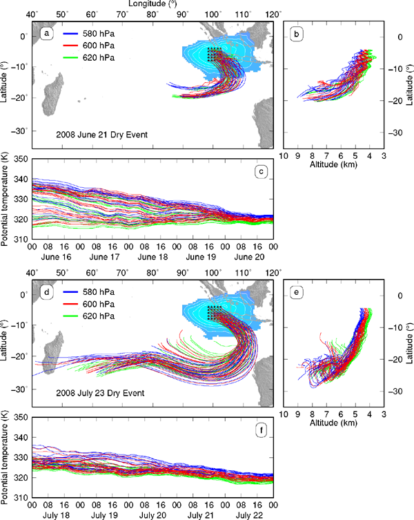
For both events, the dry-air parcels were traced back to the Southern Hemisphere between 20°S and 30°S, where the parcels first moved eastward with midlatitude westerlies, and later turned anticlockwise, advecting equatorward (Figs. 10a, d). When moving from midlatitudes to the tropics, the air parcels meanwhile subsided from the upper to middle troposphere (Figs. 10b, e). During the whole process, the potential temperature of the air parcels stayed relatively constant within 320–330 K, indicating a quasi-adiabatic process (Figs. 10c, f). For the air parcels to conserve their potential temperature, they naturally descended from the drier upper troposphere in midlatitudes to the wetter midtroposphere in the tropics. The trajectory results suggest that the REOF2 dry anomaly over southern Sumatra is a result of dry-air intrusions from the subtropics and extratropics into the tropics along the downward sloping isentropes.
To investigate what dynamical mechanism causes the observed dry-air intrusions, we applied various lags to REC2 and regressed it with the CFSR potential vorticity (PV) and winds on the 330 K isentropic surface. The results show the characteristic pattern of a Rossby wave train, with alternating areas of positive and negative PV anomalies, and strong rotational winds (Wirth et al. 2018) (Figs. 11, 12). The Rossby wave train is a continuous around-globe zonal wavenumber-6 feature that moves eastward at a phase speed of ∼ 4° longitude day−1 relative to the ground, with its latitudinal location and propagation path guided by the Southern Hemisphere westerly jet in the upper troposphere (Hoskins and Ambrizzi 1993) (Fig. 12). The vertical structure of this extratropical Rossby wave train is equivalent barotropic, as shown by in-phase anomalies throughout the troposphere (Fig. 13). The mechanism that we find here for dry-air intrusions differs from the mechanism that Fukutomi and Yasunari (2005) proposed to explain the low-level submonthly southerly surges and related dry-air intrusions over the eastern Indian Ocean, i.e., baroclinic development of midlatitude Rossby waves in the subtropical jet entrance region west of Australia. Moreover, our mechanism and the mechanism proposed by Fukutomi and Yasunari (2005) are different from Rossby wave breaking and subtropical anticyclones that have been used to explain dry-air intrusions over the tropical western Pacific (Yoneyama and Parsons 1999) and western Africa (Roca et al. 2005), respectively. In addition, dry-air intrusions have been observed over Sumatra near the equator following eastward-propagating synoptic-scale cloud systems, but these cloud systems were associated with equatorial Kelvin waves rather than extratropical Rossby waves (Murata et al. 2006).


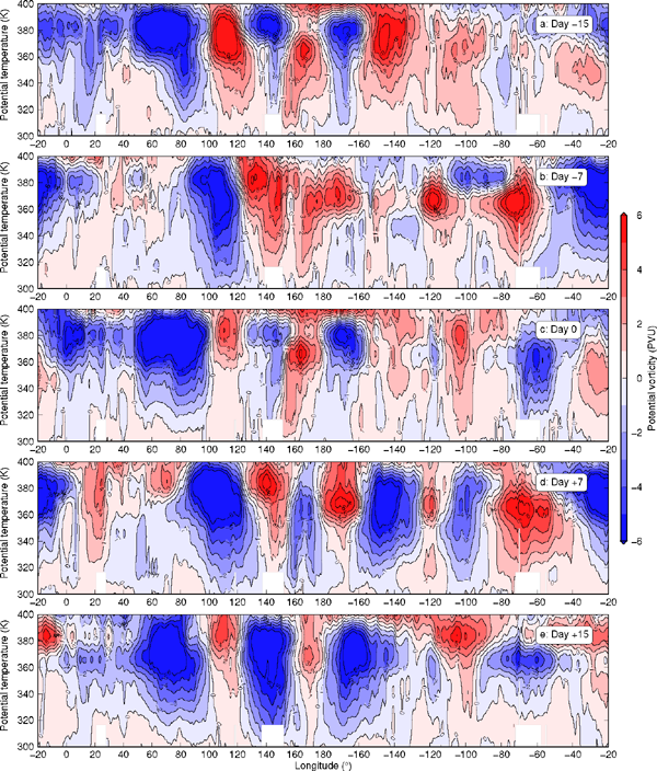
On day −15, a strong southeasterly airflow on the eastern flank of the positive PV anomaly west of Australia blows directly to southern Sumatra and Java, brings extratropical dry air, and thus causes a dry anomaly in these tropical regions (Fig. 11a). As this positive PV anomaly propagates eastward, the associated southeasterlies introduce another dry anomaly in northern Australia and the southeastern part of the Maritime Continent. Meanwhile, the dry anomaly over southern Sumatra and Java moves westward and disappears gradually (Figs. 11b–e). When the next positive PV anomaly approaches the west coast of Australia, southeasterlies blow toward southern Sumatra and Java again (Figs. 11f, g). On day 0, the positive and negative PV anomalies return to their locations on day −15, although the positive anomaly west of Australia was weaker because of weakened westerlies (Figs. 11g, 12c). The 15-day return period is consistent with the spectral peak of 15.25 days that we find in REC2. Similar quasi-biweekly variability has been observed in strong 850-hPa meridional surges over an ocean area (purple box in Fig. 12) southwest of Sumatra (Fukutomi and Yasunari 2005). The strong low-level meridional surges are likely the manifestation of midlatitude Rossby waves in the tropical lower troposphere. Note that the nature of the quasibiweekly variability that we observe here is distinct from the commonly referred quasi-biweekly mode driven by westward-propagating equatorial Rossby waves (e.g., Chatterjee and Goswami 2004).
We conclude that the second mode of the ZWD variability over Sumatra during the 2008 northern summer is controlled by the eastward-propagating quasi-biweekly fluctuation of barotropic Rossby waves originating along the Southern Hemisphere midlatitudes. When the southerlies or southeasterlies associated with positive PV anomalies are strengthened and directed to Sumatra, the SuGAr records an intense dry-air intrusion event. Our regional study also suggests that similar dry-air intrusions (shown as copperish contours in Fig. 12) can be expected to occur in other Southern Hemisphere tropical regions such as southern Maritime Continent, Australia, South America, and South Africa as long as midlatitude Rossby waves provide favorable meridional airflows. Conversely, tropical wet-air intrusions (shown as light bluish contours in Fig. 12) can be brought by the same midlatitude Rossby waves to extratropical regions.
5. How unique is the 2008 northern summer?
To test whether the South Asian Summer Monsoon and extratropical dry-air intrusions can explain the summer intra-seasonal variability of SuGAr ZWD in other years, we applied the same procedures to years ranging from 2005 to 2018. Most of the years show characteristics different from those of 2008 because they were strongly affected by inter-annual variabilities such as ENSO and IOD (not shown or discussed in this paper). However, we find that the summertime ZWD variations over Sumatra in 2016 and 2017 were also controlled by the South Asian Summer Monsoon and additionally influenced by extratropical dry-air intrusions due to midlatitude Rossby waves despite the difference in station availability (Figs. 5, S4, S5).
The 2008, 2016, and 2017 northern summers share similar horizontal and vertical extent of the REOF1 dry anomaly (Figs. 7a–c, 14a–c, 15a–c). The spatial extent of the two REOF1 wet anomalies over the monsoon regions, however, is different: for the primary wet anomaly, the 2016 one covers more oceanic region in the Arabian Sea, and the 2017 one shrinks to the northern Arabian Sea and northwestern India (Figs. 7a, 14a, 15a); for the secondary wet anomaly, the 2016 one is concentrated over the East Asian Summer Monsoon region rather than the western North Pacific Summer Monsoon region, and the 2017 one is mostly over the South China Sea (Figs. 9, 16, 17). In addition, the lag days for peak correlations between REC1 and the South Asian monsoon index or western North Pacific monsoon index differ slightly; however, the sequence that the South Asian monsoon index leads REC1 and REC1 leads the western North Pacific monsoon index does not change (Figs. 6e, 18e, 19e). The spatial and peak lag differences do not affect much the evolution of the wet, dry, and wind anomalies during a REOF1 event in which the increased activity of the South Asian Summer Monsoon likely drives more moisture over Sumatra and the eastern Indian Ocean into the western North Pacific Summer Monsoon system or even further north into the East Asian Summer Monsoon system (Figs. 9, 16, 17). The tropical western North Pacific Summer Monsoon and subtropical and extratropical East Asian Summer Monsoon are closely linked and behave relatively coherently, with the negative western North Pacific monsoon index representing well the main variability of the East Asian Summer Monsoon (Wang et al. 2008).


The REOF2 dry anomaly is also spatially similar for the three summers (Figs. 7d–f, 14d–f, 15d–f). Back trajectory results for four strong REOF2 events, two each in 2016 and 2017, show a consistent origin of the dry air in the subtropical and extratropical upper troposphere (Figs. 10, 20, 21). Interestingly, the REOF2 event on 26 July 2016 shows that the dry air could also come from northern Australia where extratropical dry-air intrusions occur likely even more frequently than those that we observe over southern Sumatra (Fig. 20a). Lead-lag regression analysis shows that the REOF2 dry events in 2016 and 2017 were also caused by Rossby waves propagating in the southern midlatitudes, but how the REOF2 dry anomaly and Rossby waves evolve during a REOF2 event is considerably different for the three summers (Figs. 11–13, S6–S11). Although the quasi-biweekly oscillation of REC2 was extremely strong in 2008, it was nonexistent in 2016 and 2017 and replaced by a broader and weaker spectral peak near the period of 10–15 days (Figs. 6d, 18d, 19d). We suspect that the Southern Hemisphere Rossby waves were so strong in 2008 that they brought frequent dry-air intrusion events to southern Sumatra and they were weaker in both 2016 and 2017 so that there were not enough events to establish the periodicity in our SuGAr data.

6. Conclusions
In this study, we used ZWD time series estimated from a regular geodetic-quality processing routine as a direct proxy for PWV to track the summer intraseasonal variability of PWV over Sumatra, and to probe the underlying atmospheric processes that control the variability. We applied rotated EOF analysis to decompose the summertime spatiotemporal field of ZWD and investigated the mechanisms behind the two most important modes. We find that the SuGAr ZWD observations during the northern summers of 2008, 2016, and 2017 shared similar features, with the variability primarily controlled by variations of the South Asian Summer Monsoon and additionally influenced by dry-air intrusions caused by Rossby waves propagating in the Southern Hemisphere midlatitudes.
Both active South Asian Summer Monsoon spells and extratropical dry-air intrusions imposed intraseasonal synoptic-scale dry anomalies over Sumatra, therefore, contributing to the dryness that Sumatra experienced during its dry season in northern summer. If these events are intense and either long-lived or frequent, they can cause droughts to develop and potentially persist in Sumatra. In Sumatra and its vicinity, droughts, particularly the severe ones, are commonly associated with modes of inter-annual variability, including the warm phase of the ENSO (El Niño), when the convection center migrates from the Maritime Continent eastward into the Pacific, and the positive phase of the IOD, when the convection center shifts westward from the eastern to western Indian Ocean (e.g., Hamada et al. 2008, 2012; Supari et al. 2018). However, our results suggest that droughts in Sumatra could also result from intra-seasonal variability induced by the active South Asian Summer Monsoon and extratropical dry-air intrusions, though more research is required to confirm the causal relationship.
Extratropical dry-air intrusions have been most extensively studied in the equatorial western Pacific (e.g., Numaguti et al. 1995; Yoneyama and Parsons 1999; Yoneyama 2003; Cau et al. 2005; Randel et al. 2016; Rieckh et al. 2017). However, extratropical dry-air intrusions in the eastern Indian Ocean and Maritime Continent have received relatively little attention to date. Using five-year relative humidity (RH) observations from the Atmospheric Infrared Sounder (AIRS) onboard the Aqua satellite, Casey et al. (2009) provided the global climatology on the occurrence, frequency, and source of dry layers (RH < 20 %) between 600 hPa and 400 hPa over warm tropical oceans. They found high-occurrence (20–40 %) of dry layers over the eastern Indian Ocean southwest of Sumatra during JJA and SON. This high-occurrence region coincides with the location of the dry anomaly of our second mode (Fig. 7d). Casey et al. (2009) also conducted back trajectory models and traced the source of midlevel dry layers over the eastern Indian Ocean back to the subtropics, but they did not provide a mechanism. Using reanalysis and OLR data, Fukutomi and Yasunari (2005) associated extratropical dry-air intrusions with low-level submonthly southerly surges over the eastern Indian Ocean and suggested baroclinic development of midlatitude Rossby waves as a mechanism. By contrast, our study with the SuGAr data suggests barotropic Rossby waves traveling in the Southern Hemisphere midlatitudes to be a possible mechanism for transporting extratropical dry air to the tropics. As the first ground-based GPS data used for studying dry-air intrusions, the local SuGAr data provide new in-situ evidence that extratropical dry-air intrusions reach the deep tropics within 5° south of the equator over the Maritime Continent. More modeling, analysis, and observation studies are required to reveal the extent, frequency, and mechanism of dry-air intrusions from the Southern Hemisphere into Southeast Asia, and their impact on tropical convections.
Supplements
Supplement 1 contains additional figures to support the main text.
Figure S1: Scatter diagram between the GIPSY-derived and MODIS-derived daily PWVs from June to September in 2008 for 22 GPS stations. Their time series are shown as black and blue lines, respectively, in Fig. 3. The MODIS thermal infrared retrievals seem to overestimate high values compared to the GIPSY-derived PWV. MODIS PWV overestimation has also been found over India (Prasad and Singh 2009).
Figure S2: Scatter diagram between the GIPSY-derived and RSS-derived daily PWVs from June to September in 2008 for 22 GPS stations. Their time series are shown as black and red lines, respectively, in Fig. 3. The GIPSY-derived and RSS-derived estimations show no clear bias.
Figure S3: Time series reconstruction using the leading two modes for the 2008 case study. Coloured lines with dots represent the daily ZWD time series we obtained for a total of 22 GPS stations. As we are interested only in variability, we added an arbitrary offset to each time series, and plot them according to their locations, roughly from north to south except NTUS. Black thin lines show the reconstructions using individual modes: (a) EC1, (b) EC2, (c) REC1 and (d) REC2.
Figure S4: Spatial pattern of EOF and rotated EOF analysis for the 32 SuGAr stations used in the northern summer 2016 study. Similar to Fig. 5.
Figure S5: Spatial pattern of EOF and rotated EOF analysis for the 25 SuGAr stations used in the northern summer 2017 study. Similar to Fig. 5.
Figure S6: Lead-lag linear regression maps for the REOF2 of the northern summer 2016. Similar to Fig. 11 but with different lags.
Figure S7: Lead-lag linear regression maps for the REOF2 of the northern summer 2017. Similar to Fig. 11 but with different lags.
Figure S8: Lead-lag linear regression maps for the REOF2 of the northern summer 2016. Similar to Fig. 12 but with different lags.
Figure S9: Lead-lag linear regression maps for the REOF2 of the northern summer 2017. Similar to Fig. 12 but with different lags.
Figure S10: Lead-lag linear regression profiles for the REOF2 of the northern summer 2016. Similar to Fig. 13 but with different lags.
Figure S11: Lead-lag linear regression profiles for 2017. Similar to Fig. 13 but with different lags.
Acknowledgments
We are deeply indebted to Prof. Kerry Sieh who was the Founding Director of the Earth Observatory of Singapore (EOS). It was his vision of establishing the SuGAr network that made this work possible. We are also very grateful to many scientists and field technicians who have helped in installing and maintaining the SuGAr network. These include Iwan Hermawan, Leong Choong Yew, Paramesh Banerjee, Jeffrey Encillo, Danny Hilman Natawidjaja, Bambang Suwargadi, Nurdin Elon Dahlan, Imam Suprihanto, Dudi Prayudi, and John Galetzka. We thank Saji N. Hameed, Nathanael Z. Wong, and Alok Bhardwaj for their useful comments on the manuscript. We thank two anonymous reviewers for their comments that improved the paper. L. F. thanks Pavel Adamek for giving useful linguistic suggestions.
This work comprises EOS contribution no. 295. This research was supported by the National Research Foundation Singapore under its NRF Investigatorship scheme (National Research Investigatorship Award No. NRF-NRFI05-2019-0009 to E.M.H.), and by the EOS via its funding from the National Research Foundation Singapore and the Singapore Ministry of Education under the Research Centers of Excellence initiative. Figures were made using Generic Mapping Tools (Wessel et al. 2013). The SuGAr daily RINEX files are available for public download at ftp://ftp.earthobservatory.sg/SugarData with a latency of three months.
References
- Aldrian, E., and R. D. Susanto, 2003: Identification of three dominant rainfall regions within Indonesia and their relationship to sea surface temperature. Int. J. Climatol., 23, 1435-1452.
- Askne, J., and H. Nordius, 1987: Estimation of tropospheric delay for microwaves from surface weather data. Radio Sci., 22, 379-386.
- Bar-Sever, Y. E., P. M. Kroger, and J. A. Borjesson, 1998: Estimating horizontal gradients of tropospheric path delay with a single GPS receiver. J. Geophys. Res., 103, 5019-5035.
- Bevis, M., S. Businger, T. A. Herring, C. Rocken, R. A. Anthes, and R. H. Ware, 1992: GPS meteorology: Remote sensing of atmospheric water vapor using the global positioning system. J. Geophys. Res., 97, 15787-15801.
- Bevis, M., S. Businger, S. Chiswell, T. A. Herring, R. A. Anthes, C. Rocken, and R. H. Ware, 1994: GPS meteorology: Mapping zenith wet delays onto precipitable water. J. Appl. Meteor., 33, 379-386.
- Blewitt, G., W. C. Hammond, and C. Kreemer, 2018: Harnessing the GPS data explosion for interdisciplinary science. Eos, 99, doi:10.1029/2018EO104623.
- Bock, O., F. Guichard, S. Janicot, J. P. Lafore, M.-N. Bouin, and B. Sultan, 2007: Multiscale analysis of precipitable water vapor over Africa from GPS data and ECMWF analyses. Geophys. Res. Lett., 34, L09705, doi:10.1029/2006GL028039.
- Bock, O., M. N. Bouin, E. Doerflinger, P. Collard, F. Masson, R. Meynadier, S. Nahmani, M. Koité, K. Gaptia Lawan Balawan, F. Didé, D. Ouedraogo, S. Pokperlaar, J.-B. Ngamini, J. P. Lafore, S. Janicot, F. Guichard, and M. Nuret, 2008: West African Monsoon observed with ground-based GPS receivers during African Monsoon Multidisciplinary Analysis (AMMA). J. Geophys. Res., 113, D21105, doi:10.1029/2007JD010327.
- Boehm, J., B. Werl, and H. Schuh, 2006: Troposphere mapping functions for GPS and very long baseline interferometry from European Centre for Medium-Range Weather Forecasts operational analysis data. J. Geophys. Res., 111, B02406, doi:10.1029/2005JB003629.
- Cadet, D., and G. Reverdin, 1981: Water vapour transport over the Indian Ocean during summer 1975. Tellus, 33, 476-487.
- Casey, S. P. F., A. E. Dessler, and C. Schumacher, 2009: Five-year climatology of midtroposphere dry air layers in warm tropical ocean regions as viewed by AIRS/Aqua. J. Appl. Meteor. Climatol., 48, 1831-1842.
- Cau, P., J. Methven, and B. Hoskins, 2005: Representation of dry tropical layers and their origins in ERA-40 data. J. Geophys. Res., 110, D06110, doi:10.1029/2004JD004928.
- Chang, C.-P., Z. Wang, J. McBride, and C.-H. Liu, 2005: Annual cycle of Southeast Asia-Maritime Continent rainfall and the asymmetric monsoon transition. J. Climate, 18, 287-301.
- Chatterjee, P., and B. N. Goswami, 2004: Structure, genesis and scale selection of the tropical quasi-biweekly mode. Quart. J. Roy. Meteor. Soc., 130, 1171-1194.
- Dai, A., J. Wang, R. H. Ware, and T. Van Hove, 2002: Diurnal variation in water vapor over North America and its implications for sampling errors in radiosonde humidity. J. Geophys. Res., 107, 4090, doi:10.1029/2001JD000642.
- Davis, J. L., T. A. Herring, I. I. Shapiro, A. E. E. Rogers, and G. Elgered, 1985: Geodesy by radio interferometry: Effects of atmospheric modeling errors on estimates of baseline length. Radio Sci., 20, 1593-1607.
- Davis, J. L., G. Elgered, A. E. Niell, and C. E. Kuehn, 1993: Ground-based measurement of gradients in the “wet” radio refractivity of air. Radio Sci., 28, 1003-1018.
- Dee, D. P., S. M. Uppala, A. J. Simmons, P. Berrisford, P. Poli, S. Kobayashi, U. Andrae, M. A. Balmaseda, G. Balsamo, P. Bauer, P. Bechtold, A. C. M. Beljaars, L. van de Berg, J. Bidlot, N. Bormann, C. Delsol, R. Dragani, M. Fuentes, A. J. Geer, L. Haimberger, S. B. Healy, H. Hersbach, E. V. Hólm, L. Isaksen, P. Kållberg, M. Köhler, M. Matricardi, A. P. McNally, B. M. Monge-Sanz, J.-J. Morcrette, B.-K. Park, C. Peubey, P. de Rosnay, C. Tavolato, J.-N. Thépaut, and F. Vitart, 2011: The ERA-Interim reanalysis: configuration and performance of the data assimilation system. Quart. J. Roy. Meteor. Soc., 137, 553-597.
- Feng, L., E. M. Hill, P. Banerjee, I. Hermawan, L. L. H. Tsang, D. H. Natawidjaja, B. W. Suwargadi, and K. Sieh, 2015: A unified GPS-based earthquake catalog for the Sumatran plate boundary between 2002 and 2013. J. Geophys. Res.: Solid Earth, 120, 3566-3598.
- Findlater, J., 1969a: A major low-level air current near the Indian Ocean during the northern summer. Quart. J. Roy. Meteor. Soc., 95, 362-380.
- Findlater, J., 1969b: Interhemispheric transport of air in the lower troposphere over the western Indian Ocean. Quart. J. Roy. Meteor. Soc., 95, 400-403.
- Fujita, M., K. Yoneyama, S. Mori, T. Nasuno, and M. Satoh, 2011: Diurnal convection peaks over the eastern Indian Ocean off Sumatra during different MJO phases. J. Meteor. Soc. Japan, 89A, 317-330.
- Fukutomi, Y., and T. Yasunari, 2005: Southerly surges on submonthly time scales over the eastern Indian Ocean during the Southern Hemisphere winter. Mon. Wea. Rev., 133, 1637-1654.
- Gilman, D. L., F. J. Fuglister, and J. M. Mitchell, Jr., 1963: On the power spectrum of “red noise”. J. Atmos. Sci., 20, 182-184.
- Guerova, G., J. Jones, J. Douša, G. Dick, S. de Haan, E. Pottiaux, O. Bock, R. Pacione, G. Elgered, H. Vedel, and M. Bender, 2016: Review of the state of the art and future prospects of the ground-based GNSS meteorology in Europe. Atmos. Meas. Tech., 9, 5385-5406.
- Hamada, J.-I., M. D. Yamanaka, J. Matsumoto, S. Fukao, P. A. Winarso, and T. Sribimawati, 2002: Spatial and temporal variations of the rainy season over Indonesia and their link to ENSO. J. Meteor. Soc. Japan, 80, 285-310.
- Hamada, J.-I., M. D. Yamanaka, S. Mori, Y. I. Tauhid, and T. Sribimawati, 2008: Differences of rainfall characteristics between coastal and interior areas of central western Sumatera, Indonesia. J. Meteor. Soc. Japan, 86, 593-611.
- Hamada, J.-I., S. Mori, H. Kubota, M. D. Yamanaka, U. Haryoko, S. Lestari, R. Sulistyowati, and F. Syamsudin, 2012: Interannual rainfall variability over northwestern Jawa and its relation to the Indian Ocean Dipole and El Niño-Southern Oscillation events. SOLA, 8, 69-72.
- Hannachi, A., I. T. Jolliffe, and D. B. Stephenson, 2007: Empirical orthogonal functions and related techniques in atmospheric science: A review. Int. J. Climatol., 27, 1119-1152.
- Hattori, M., K. Tsuboki, and T. Takeda, 2005: Interannual variation of seasonal changes of precipitation and moisture transport in the western North Pacific. J. Meteor. Soc. Japan, 83, 107-127.
- Heckley, W. A., and A. E. Gill, 1984: Some simple analytical solutions to the problem of forced equatorial long waves. Quart. J. Roy. Meteor. Soc., 110, 203-217.
- Hendon, H. H., 2003: Indonesian rainfall variability: Impacts of ENSO and local airsea interaction. J. Climate, 16, 1775-1790.
- Hopfield, H. S., 1971: Tropospheric range error at the zenith. Technical report, Johns Hopkins University. [Available at https://apps.dtic.mil/dtic/tr/fulltext/u2/749669.pdf.].
- Hoskins, B. J., and T. Ambrizzi, 1993: Rossby wave propagation on a realistic longitudinally varying flow. J. Atmos. Sci., 50, 1661-1671.
- Joseph, P. V., and S. Sijikumar, 2004: Intraseasonal variability of the low-level jet stream of the Asian summer monsoon. J. Climate, 17, 1449-1458.
- Joseph, P. V., K. P. Sooraj, and C. K. Rajan, 2006: The summer monsoon onset process over South Asia and an objective method for the date of monsoon onset over Kerala. Int. J. Climatol., 26, 1871-1893.
- Kaiser, H. F., 1958: The varimax criterion for analytic rotation in factor analysis. Psychometrika, 23, 187-200.
- Kämpfer, N., 2013: Monitoring Atmospheric Water Vapour: Ground-Based Remote Sensing and In-situ Methods. ISSI Scientific Report Series book series (ISSI, volume 10), Springer, New York, USA, 328 pp.
- King, M. D., W. P. Menzel, Y. J. Kaufman, D. Tanre, B.-C. Gao, S. Platnick, S. A. Ackerman, L. A. Remer, R. Pincus, and P. A. Hubanks, 2003: Cloud and aerosol properties, precipitable water, and profiles of temperature and water vapor from MODIS. IEEE Trans. Geosci. Remote Sens., 41, 442-458.
- Lindzen, R. S., and S. Nigam, 1987: On the role of sea surface temperature gradients in forcing low-level winds and convergence in the tropics. J. Atmos. Sci., 44, 2418-2436.
- Manandhar, S., Y. H. Lee, Y. S. Meng, and J. T. Ong, 2017: A simplified model for the retrieval of precipitable water vapor from GPS signal. IEEE Trans. Geosci. Remote Sens., 55, 6245-6253.
- Mears, C. A., J. Wang, D. Smith, and F. J. Wentz, 2015: Intercomparison of total precipitable water measurements made by satellite-borne microwave radiometers and ground-based GPS instruments. J. Geophys. Res.: Atmos., 120, 2492-2504.
- Murakami, T., J. Matsumoto, and A. Yatagai, 1999: Similarities as well as differences between summer monsoons over Southeast Asia and the western North Pacific. J. Meteor. Soc. Japan, 77, 887-906.
- Murata, F., M. D. Yamanaka, H. Hashiguchi, S. Mori, M. Kudsy, T. Sribimawati, B. Suhardi, and Emrizal, 2006: Dry intrusions following eastward-propagating synoptic-scale cloud systems over Sumatera Island. J. Meteor. Soc. Japan, 84, 277-294.
- Niell, A. E., 1996: Global mapping functions for the atmosphere delay at radio wavelengths. J. Geophys. Res., 101, 3227-3246.
- Nilsson, T., and G. Elgered, 2008: Long-term trends in the atmospheric water vapor content estimated from ground-based GPS data. J. Geophys. Res., 113, D19101, doi:10.1029/2008JD010110.
- Ninomiya, K., 1999: Moisture balance over China and the South China Sea during the summer monsoon in 1991 in relation to the intense rainfalls over China. J. Meteor. Soc. Japan, 77, 737-751.
- Numaguti, A., R. Oki, K. Nakamura, K. Tsuboki, N. Misawa, T. Asai, and Y.-M. Kodama, 1995: 4-5-day-period variation and low-level dry air observed in the equatorial western Pacific during the TOGA-COARE IOP. J. Meteor. Soc. Japan, 73, 267-290.
- Okamoto, N., M. D. Yamanaka, S.-Y. Ogino, H. Hashiguchi, N. Nishi, T. Sribimawati, and A. Numaguti, 2003: Seasonal variations of tropospheric wind over Indonesia: Comparison between collected operational rawinsonde data and NCEP reanalysis for 1992-99. J. Meteor. Soc. Japan, 81, 829-850.
- Pai, D. S., L. Sridhar, and M. R. Ramesh Kumar, 2016: Active and break events of Indian summer monsoon during 1901–2014. Climate Dyn., 46, 3921-3939.
- Poan, D. E., R. Roehrig, F. Couvreux, and J.-P. Lafore, 2013: West African monsoon intraseasonal variability: A precipitable water perspective. J. Atmos. Sci., 70, 1035-1052.
- Pramualsakdikul, S., R. Haas, G. Elgered, and H.-G. Scherneck, 2007: Sensing of diurnal and semi-diurnal variability in the water vapour content in the tropics using GPS measurements. Meteor. Appl., 14, 403-412.
- Prasad, A. K., and R. P. Singh, 2009: Validation of MODIS Terra, AIRS, NCEP/DOE AMIP-II Reanalysis-2, and AERONET Sun photometer derived integrated precipitable water vapor using ground-based GPS receivers over India. J. Geophys. Res., 114, D05107, doi:10.1029/2008JD011230.
- Qian, J.-H., 2008: Why precipitation is mostly concentrated over islands in the Maritime Continent. J. Atmos. Sci., 65, 1428-1441.
- Rajeevan, M., S. Gadgil, and J. Bhate, 2010: Active and break spells of the Indian summer monsoon. J. Earth Syst. Sci., 119, 229-247.
- Ramage, C. S., 1968: Role of a tropical “maritime continent" in the atmospheric circulation. Mon. Wea. Rev., 96, 365-370.
- Randel, W. J., L. Rivoire, L. L. Pan, and S. B. Honomichl, 2016: Dry layers in the tropical troposphere observed during CONTRAST and global behavior from GFS analyses. J. Geophys. Res.: Atmos., 121, 14142-14158.
- Richman, M. B., 1986: Rotation of principal components. J. Climatol., 6, 293-335.
- Rieckh, T., R. Anthes, W. Randel, S.-P. Ho, and U. Foelsche, 2017: Tropospheric dry layers in the tropical western Pacific: Comparisons of GPS radio occultation with multiple data sets. Atmos. Meas. Tech., 10, 1093-1110.
- Roca, R., J.-P. Lafore, C. Piriou, and J.-L. Redelsperger, 2005: Extratropical dry-air intrusions into the West African monsoon midtroposphere: An important factor for the convective activity over the Sahel. J. Atmos. Sci., 62, 390-407.
- Rolph, G., A. Stein, and B. Stunder, 2017: Real-time Environmental Applications and Display sYstem: READY. Environ. Modell. Software, 95, 210-228.
- Saastamoinen, J., 1972: Atmospheric correction for the troposphere and stratosphere in radio ranging satellites. The Use of Artificial Satellittes for Geodesy. Geophys. Monogr. Ser., Henriksen, S. W., A. Mancini, and B. H. Chovitz, (eds.), American Geophysical Union, Washington, D. C., 247-251.
- Saha, K., 1970: Air and water vapour transport across the equator in western Indian Ocean during northern summer. Tellus, 22, 681-687.
- Saha, S., S. Moorthi, H.-L. Pan, X. Wu, J. Wang, S. Nadiga, P. Tripp, R. Kistler, J. Woollen, D. Behringer, H. Liu, D. Stokes, R. Grumbine, G. Gayno, J. Wang, Y.-T. Hou, H.-Y. Chuang, H.-M. H. Juang, J. Sela, M. Iredell, R. Treadon, D. Kleist, P. Van Delst, D. Keyser, J. Derber, M. Ek, J. Meng, H. Wei, R. Yang, S. Lord, H. van den Dool, A. Kumar, W. Wang, C. Long, M. Chelliah, Y. Xue, B. Huang, J.-K. Schemm, W. Ebisuzaki, R. Lin, P. Xie, M. Chen, S. Zhou, W. Higgins, C.-Z. Zou, Q. Liu, Y. Chen, Y. Han, L. Cucurull, R. W. Reynolds, G. Rutledge, and M. Goldberg, 2010: The NCEP Climate Forecast System Reanalysis. Bull. Amer. Meteor. Soc., 91, 1015-1058.
- Saji, N. H., B. N. Goswami, P. N. Vinayachandran, and T. Yamagata, 1999: A dipole mode in the tropical Indian Ocean. Nature, 401, 360-363.
- Spilker, J. J., 1996: Tropospheric effects on GPS. Global Positioning System: Theory and Applications. Parkinson, B. W., and J. J. Spilker (eds.), The American Institute of Aeronautics and Astronautics, Washington, D.C., 517-546.
- Srinivasan, J., and R. S. Nanjundiah, 2002: The evolution of Indian summer monsoon in 1997 and 1983. Meteor. Atmos. Phys., 79, 243-257.
- Stein, A. F., R. R. Draxler, G. D. Rolph, B. J. B. Stunder, M. D. Cohen, and F. Ngan, 2015: NOAA's HYSPLIT atmospheric transport and dispersion modeling system. Bull. Amer. Meteor. Soc., 96, 2059-2077.
- Supari, F. Tangang, E. Salimun, E. Aldrian, A. Sopaheluwakan, and L. Juneng, 2018: ENSO modulation of seasonal rainfall and extremes in Indonesia. Climate Dyn., 51, 2559-2580.
- Susskind, J., C. D. Barnet, and J. M. Blaisdell, 2003: Retrieval of atmospheric and surface parameters from AIRS/AMSU/HSB data in the presence of clouds. IEEE Trans. Geosci. Remote Sens., 41, 390-409.
- Torri, G., D. K. Adams, H. Wang, and Z. Kuang, 2019: On the diurnal cycle of GPS-derived precipitable water vapor over Sumatra. J. Atmos. Sci., 76, 3529-3552.
- Tralli, D. M., and S. M. Lichten, 1990: Stochastic estimation of tropospheric path delays in Global Positioning System geodetic measurements. Bulletin Géodésique, 64, 127-159.
- Tralli, D. M., T. H. Dixon, and S. A. Stephens, 1988: Effect of wet tropospheric path delays on estimation of geodetic baselines in the Gulf of California using the Global Positioning System. J. Geophys. Res., 93, 6545-6557.
- Ueda, H., T. Yasunari, and R. Kawamura, 1995: Abrupt seasonal change of large-scale convective activity over the western Pacific in the northern summer. J. Meteor. Soc. Japan, 73, 795-809.
- Wang, B., and Z. Fan, 1999: Choice of South Asian summer monsoon indices. Bull. Amer. Meteor. Soc., 80, 629-638.
- Wang, B., and LinHo, 2002: Rainy season of the Asian-Pacific summer monsoon. J. Climate, 15, 386-398.
- Wang, B., R. Wu, and K.-M. Lau, 2001: Interannual variability of the Asian summer monsoon: Contrasts between the Indian and the western North Pacific-East Asian Monsoons. J. Climate, 14, 4073-4090.
- Wang, J., L. Zhang, A. Dai, T. Van Hove, and J. Van Baelen, 2007: A near-global, 2-hourly data set of atmospheric precipitable water from ground-based GPS measurements. J. Geophys. Res., 112, D11107, doi:10.1029/2006JD007529.
- Wang, B., Z. Wu, J. Li, J. Liu, C.-P. Chang, Y. Ding, and G. Wu, 2008: How to measure the strength of the East Asian summer monsoon. J. Climate, 21, 4449-4463.
- Wang, J., A. Dai, and C. Mears, 2016: Global water vapor trend from 1988 to 2011 and its diurnal asymmetry based on GPS, radiosonde, and microwave satellite measurements. J. Climate, 29, 5205-5222.
- Wentz, F. J., 1997: A well-calibrated ocean algorithm for special sensor microwave/imager. J. Geophys. Res., 102, 8703-8718.
- Wentz, F. J., 2013: SSM/I Version-7 calibration report. RSS Technical Report 011012, Remote Sensing Systems, Santa Rosa, CA, 46 pp. [Available at https://ghrc.nsstc.nasa.gov/pub/doc/ssmi_netcdf/2012_Wentz_011012_Version-7_SSMI_Calibration.pdf.]
- Wessel, P., W. H. F. Smith, R. Scharroo, J. Luis, and F. Wobbe, 2013: Generic Mapping Tools: Improved version released. Eos, Trans. Amer. Geophys. Union, 94, 409-410.
- Wilson, S. S., K. Mohanakumar, and S. Roose, 2019: A study on the structural transformation of the monsoon low-level jet stream on its passage over the South Asian region. Pure Appl. Geophys., 176, 3681-3695.
- Wirth, V., M. Riemer, E. K. M. Chang, and O. Martius, 2018: Rossby wave packets on the midlatitude waveguide-A review. Mon. Wea. Rev., 146, 1965-2001.
- Wu, P., J.-I. Hamada, S. Mori, Y. I. Tauhid, M. D. Yamanaka, and F. Kimura, 2003: Diurnal variation of precipitable water over a mountainous area of Sumatra Island. J. Appl. Meteor., 42, 1107-1115.
- Wu, P., S. Mori, J.-I. Hamada, M. D. Yamanaka, J. Matsumoto, and F. Kimura, 2008: Diurnal variation of rainfall and precipitable water over Siberut Island off the western coast of Sumatra Island. SOLA, 4, 125-128.
- Wulfmeyer, V., R. M. Hardesty, D. D. Turner, A. Behrendt, M. P. Cadeddu, P. Di Girolamo, P. Schlüssel, J. Van Baelen, and F. Zus, 2015: A review of the remote sensing of lower tropospheric thermodynamic profiles and its indispensable role for the understanding and the simulation of water and energy cycles. Rev. Geophys., 53, 819-895.
- Yamanaka, M. D., 2016: Physical climatology of Indonesian maritime continent: An outline to comprehend observational studies. Atmos. Res., 178-179, 231-259.
- Yamanaka, M. D., S.-Y. Ogino, P.-M. Wu, J.-I. Hamada, S. Mori, J. Matsumoto, and F. Syamsudin, 2018: Maritime continent coastlines controlling Earth's climate. Prog. Earth Planet. Sci., 5, 21, doi:10.1186/s40645-018-0174-9.
- Yim, S.-Y., B. Wang, J. Liu, and Z. Wu, 2014: A comparison of regional monsoon variability using monsoon indices. Climate Dyn., 43, 1423-1437.
- Yoneyama, K., 2003: Moisture variability over the tropical western Pacific Ocean. J. Meteor. Soc. Japan, 81, 317-337.
- Yoneyama, K., and D. B. Parsons, 1999: A proposed mechanism for the intrusion of dry air into the tropical western Pacific region. J. Atmos. Sci., 56, 1524-1546.
- Zangvil, A., 1977: On the presentation and interpretation of spectra of large-scale disturbances. Mon. Wea. Rev., 105, 1469-1472.
- Zumberge, J. F., M. B. Heflin, D. C. Jefferson, M. M. Watkins, and F. H. Webb, 1997: Precise point positioning for the efficient and robust analysis of GPS data from large networks. J. Geophys. Res., 102, 5005-5017.