Tropical Cyclones in Global Storm-Resolving Models

Abstract

Recent progress in computing and model development has initiated the era of global storm-resolving modeling, and with it the potential to transform weather and climate prediction. Within the general theme of vetting this new class of models, the present study evaluates nine global-storm resolving models in their ability to simulate tropical cyclones (TCs). Results indicate that, broadly speaking, the models produce realistic TCs and remove longstanding issues known from global models such as the deficiency in accurately simulating TC intensity. However, TCs are strongly affected by model formulation, and all models suffer from unique biases regarding the number of TCs, intensity, size, and structure. Some models simulated TCs better than others, but no single model was superior in every way. The overall results indicate that global storm-resolving models can open a new chapter in TC prediction, but they need to be improved to unleash their full potential.

1. Introduction

Tropical cyclones (TCs) are among the most destructive natural hazards, and predicting TCs is an important task of weather and climate models. Moreover, TCs are optimal testbeds for assessing the quality of numerical models, because their unique dynamics reveal deficiencies in the model formulation through artifacts such as unrealistic structure. The overall purpose of the present study is to evaluate a new class of atmosphere models—global storm-resolving models¹ (Satoh et al. 2019)—in their ability to simulate TCs. Specifically, we report on TC-related achievements, deficiencies, and biases in nine global storm-resolving models, and we hope that our findings will pave the way for improving the next generation of weather and climate models.

Global models have been a vital instrument in TC prediction although they have not been able to accurately predict TC intensity. A decade ago, Hamill et al. (2011) reported that global weather models, which at that time had mesh spacings between 50 km and 150 km, were plagued by wind speed biases of down to −30 m s⁻¹. Even though some progress has been made, the most recent models with mesh spacings between 10 km and 25 km still fail to capture the high winds of TCs (e.g., Magnusson et al. 2019; Hodges and Klingaman 2019; Roberts et al. 2020). One of the main reasons for this shortcoming is insufficient horizontal resolution (Davis 2018). In fact, years of research with regional models have indicated that storm-resolving resolution (here defined as ≤ 5 km) is necessary for accurate simulation of the inner-core structure of TCs (e.g., Chen et al. 2007; Gentry and Lackmann 2010), which in turn is necessary to predict TC intensity (e.g., Davis et al. 2008; Gopalakrishnan et al. 2012; Fox and Judt 2018).

The preceding paragraph suggests that global storm-resolving models are ideal tools for TC prediction, because they combine the advantages of current-generation global and regional models, that is, they offer global coverage and storm-resolving horizontal resolution. Indeed, there has been some qualitative evidence that global storm-resolving models capture the inner-core structure of TCs quite realistically (e.g., Fudeyasu et al. 2008; Zhou et al. 2019). Other studies have demonstrated that models with 7–10 km mesh spacings reduce some of the biases found in coarser-resolution models (Manganello et al. 2012; Nakano et al. 2017). However, the immense computational resources required to run global models with mesh spacings ≤ 5 km have so far precluded a detailed, TC-focused evaluation of those models. The present study attempts to fill this gap by evaluating the models that participated in the DYnamics of the Atmospheric general circulation Modeled On Non-hydrostatic Domains (DYAMOND) initiative (Stevens et al. 2019), and it expands on the brief overview of TCs already presented in Stevens et al. (2019).

Given computational limitations and the general purpose of DYAMOND, it was not possible to evaluate the models as typically done in the weather prediction community, i.e., by computing errors of metrics such as maximum wind speed from a large number of short-range forecasts (e.g., DeMaria et al. 2014; Nakano et al. 2017). It was also not possible to evaluate long-term TC climatologies as in climate studies (e.g., Camargo et al. 2005; Bengtsson et al. 2007; Manganello et al. 2012; Roberts et al. 2020). Instead, we focused on answering the following questions:

• ・What are the biases in TC number, tracks, intensity, and size over the 40-day DYAMOND period?
• ・Do the models produce TCs with a realistic structure?
• ・Do the models have similar biases, or does each model have its own?

The validity of the study rests on three important assumptions, namely (i) The 40-day DYAMOND period is sufficient to draw general conclusions about the TC characteristics in each model; (ii) objects identified as TCs by the tracking software (see Section 2) would also be identified as TCs by human forecasters—and vice versa; and (iii) the observations used to evaluate the models are sufficiently accurate.

We are confident that (i) holds true because the discrepancies between the models were substantial and almost certainly caused by different model formulations. Furthermore, even though 40 days is relatively short, we have global statistics, and the sampling is not as sparse as one might intuit. It is more difficult to judge the validity of (ii) and (iii), but given the amount of past studies that relied on those assumptions, we assumed they would also hold for this work.

Lastly, we emphasize that high horizontal resolution is necessary but not sufficient for accurately simulating TCs. Advances in ocean coupling and model physics are critical as well (e.g., Lee and Chen 2014; Mogensen et al. 2017; Magnusson et al. 2019). One area that seems to be particularly important is the parameterization of the boundary layer (Kanada et al. 2012; Kepert 2012; Zhang et al. 2015) and the surface layer, especially the surface momentum fluxes (Zeng et al. 2010; Green and Zhang 2013; Magnusson et al. 2019).

The remainder of the paper is structured as follows: in Section 2, we present the data and methods. Section 3 contains the results, organized into subsections on (i) TC number and tracks, (ii) intensity, (iii) size, (iv) structure, and (v) the sensitivity of TCs on resolution and parameterized convection. The findings are discussed in Section 4 and the paper ends with a summary and conclusions in Section 5.

2. Data and methods

This study leverages the vast data repository of DYAMOND, which contains the output from the following nine global models: ARPEGE, FV3, GEOS, ICON, IFS², MPAS, NICAM, SAM, and UM. The horizontal resolution of the models is given in Table 1. All models except GEOS were initialized with the 00 UTC 1 August 2016 analysis from the European Centre for Medium-Range Weather Forecasts (ECMWF) and integrated for 40 days (1 August–10 September 2016). The sea surface temperature and sea ice fields were prescribed using 7-day running mean analyses from ECMWF. For more information about the DYAMOND experiment and the participating models see Stevens et al. (2019) and references therein.

To identify TCs in the model output, we employed the GFDL vortex tracker (Marchok 2002; Biswas et al. 2018). This software uses the following iterative process to provide TC position fixes: First, the tracker employs a single-pass Barnes analysis to determine the location of extrema in each of the following variables: relative vorticity at 10 m (maximum), sea-level pressure (minimum), wind speed at 10 m (minimum), relative vorticity at 850 hPa and 700 hPa (maximum), and wind speed at 850 hPa and 700 hPa (minimum). After the first iteration, additional iterations are performed. For each additional iteration, the Barnes analysis grid is centered on the center fixes from the previous iteration, and the grid spacing of the analysis grid is halved to obtain fixes on a grid that is as fine as possible. The center fixes for all parameters are then averaged to produce a mean TC center position.

The tracker produces track files with 6-hourly records that contain TC location (latitude/longitude), maximum 10-m wind speed (v_max), minimum sea-level pressure (p_min), and wind radii r₁₇, r₂₅, and r₃₂, i.e., the maximum radial extent of 17, 25, and 32 m s⁻¹ winds in each compass quadrant (northeast, southeast, southwest, and northwest). A warm core criterion is applied, and tracks are discarded if a local maximum in the 300–500 hPa layer's mean temperature is not present for at least 50 % of a given storm's lifetime.

To evaluate the models, we used best track data from the International Best Track Archive for Climate Stewardship [IBTrACS version 4; Knapp et al. (2010, 2018)] for the 40-day DYAMOND period. Specifically, we used the “official” data from the Tropical Cyclone Regional Specialized Meteorological Centres that are responsible for detecting TCs in their designated area of responsibility (e.g., the National Hurricane Center for Atlantic and Eastern Pacific TCs), and we accounted for wind speed reporting differences by converting all v_max values to 1-min sustained winds following Harper et al. (2008). Note that the IBTrACS data do not contain direct observations or objective analyses, but subjective analyses from human forecasters based on available but limited observations. For simplicity, we nevertheless refer to the IBTrACS data as “observations”. Furthermore, we make the assumption that the IBTrACS v_max values are equivalent to the simulated maximum instantaneous wind. According to Nolan et al. (2009), this may be a valid assumption at 1.33-km grid spacing, but at coarser resolution, the model instantaneous wind is somewhat less than a 1-min sustained wind.

For a number of reasons, the work flow was not trivial. For example, some groups provided the output on their native model mesh, which rendered the data unreadable for the tracker. Furthermore, the high-resolution output caused the tracker to falsely identify hundreds of convective objects as TCs. To overcome those issues, we carried out the following three-step process:

• 1. Interpolate the output from each model to a common longitude/latitude grid with 0.5° resolution.
• 2. Run the tracker on the interpolated grids. Keep in mind that the track files contain information from the smoothed data.
• 3. Use the storm center information from step 2 to search for the actual v_max, p_min, r₁₇, r₂₅, and r₃₂ in the native model files, and overwrite the data in the track files with these new values.

Even after this process, the software tracked objects that human meteorologists would not identify as TCs, such as disorganized convective systems and heat lows over the deserts of Iran and central Asia. To reduce the number of falsely-identified objects as much as possible, the track files were quality-controlled using the following criteria:

• ・Drop all storms that form inland over Arabia and Iran.
• ・Drop all storms with lifetimes under 48 h.
• ・Drop all storms that never achieved a v_max of 7.5 m s⁻¹.
• ・Drop all records poleward of ±40° latitude (i.e., remove extratropical transitions).

The IBTrACS data were quality-controlled using the same criteria to homogenize model data and observations. The final quality-controlled track files from the DYAMOND models can be obtained from Judt et al. (2020).

3. Results

3.1 Number of tropical cyclones and tracks

Meteorological services observed a global total of 24 TCs during the 40-day DYAMOND period, whereas the models simulated between 12 and 31 TCs, i.e., 50–140 % of the observed value (Fig. 1). Most of the models simulated fewer TCs than observed; specifically, six of the nine models (ARPEGE, FV3, ICON, IFS, MPAS, and SAM) simulated less than 24 TCs (Figs. 1b, c, e–g, i), and only NICAM and UM simulated more TCs than observed (Figs. 1h, j). GEOS simulated exactly 24 TCs (Fig. 1d), however, considering the limited sample size and the likelihood that a different tracker may have yielded slightly different numbers, we do not wish to emphasize the exact number of TCs each model produced.

Fig. 1.

TC tracks and numbers from observations (black/grey) and models (orange) for the DYAMOND period (1 August–10 September 2016). Numbers are given for each basin (Indian Ocean, Western Pacific, Eastern Pacific, Atlantic); the global total number of TCs is shown in the lower right.

According to the observations, the Western Pacific was the most active basin during the DYAMOND time period, followed by the Eastern Pacific, Atlantic, and Indian Oceans. All models agreed that the Western Pacific was going to be the most active basin, and the simulated tracks were generally oriented from south to north as in the observations (Fig. 1). However, the models were not as successful in the other basins. For example, in the Eastern Pacific, all models, except MPAS (Fig. 1g), simulated fewer TCs than observed, and in most models there was less agreement between the orientation of the observed and simulated tracks. FV3 seems to have done best in terms of tracks in this basin (Fig. 1c). TC activity in the Atlantic proved to be particularly difficult to capture, and some models simulated a very active basin while others simulated a very quiet one. Specifically, NICAM produced 11 Atlantic TCs (Fig. 1h), whereas FV3 and IFS only produced one (Figs. 1c, f).

TC formation events during the DYAMOND period were not spread out uniformly over time but occurred in more or less well-defined periods (Fig. 2, black dots). The models simulated the temporal modulation of activity in rough agreement with the observations. For example, in the Western Pacific, most models correctly simulated a greater number of formation events before 22 August than after that date (Fig. 2a). In the Eastern Pacific, the models missed some of the formation events in early August, but they agreed with the observations on a second round of activity in late August/early September (Fig. 2b). In the Atlantic, about half of the models suggested a relatively active period in mid/late August, around the same time four formation events were observed (Fig. 2c). By contrast, the models struggled with capturing the timing of TC formation in the Indian Ocean (Fig. 2d); however, with only two observed events, this basin is likely not representative.

Fig. 2.

Timeseries of TC formation events in the Western Pacific (a), Eastern Pacific (b), Atlantic (c), and Indian Ocean (d) from observations (black) and models (orange).

At this point we can only speculate why the models were able to capture the temporal modulation of activity beyond the typical predictability limit of weather prediction, which is around two weeks. One possible reason is that the models were able to capture the modulating effect of intraseasonal variability as previously demonstrated by Nakano et al. (2015). Another possible reason is that the prescribed sea-surface temperatures artificially impart longer predictability on the atmosphere.

Perhaps most importantly, Fig. 2 demonstrates that no model suffered from a climate drift; that is, no model showed the number of TC formation events to unrealistically increase or decrease over the 40-day period. This highlights the quality of the DYAMOND models, which were not tuned for the experiment.

As a final remark, we note that UM produced a three member mini-ensemble instead of a single simulation. The differences in TC numbers and tracks within this ensemble were as large as (or at times larger) than inter-model differences (not shown). This indicates that more simulations and ensemble runs are required to properly assess the predictive skill of each model beyond the broad statements made earlier.

3.2 Tropical cyclone intensity

Time series of v_max in Fig. 3 provide a broad overview of the intensity of the TCs and allow for a cursory model evaluation. Some biases are evident; for example, ICON and SAM produced storms that were generally too weak (Figs. 3e, i), whereas ARPEGE produced a few storms that were much too strong. In fact, ARPEGE produced storms with unrealistically high v_max of > 100 m s⁻¹ (Fig. 3b), most likely because the evaporation coefficient was set to a wrong value (Stevens et al. 2019).

Fig. 3.

Timeseries of maximum surface wind speed (v_max) for each TC from observations (black, grey) and models (orange).

According to the observations, the TCs during the first 2 weeks of August remained relatively weak with only two storms reaching hurricane intensity (v_max ≥ 33 m s⁻¹; Fig. 3a). By contrast, some of the TCs that formed in the second half of August became quite intense, with four storms reaching major hurricane intensity (v_max ≥ 50 m s⁻¹). Most models had issues with capturing this pattern. Specifically, a number of models simulated storms in the first half of August that were too intense (ARPEGE, GEOS, NICAM, UM; Figs. 3b, d, h, j). From all models, MPAS seems to have best captured the overall pattern (Fig. 3g).

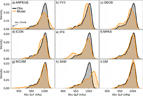
To evaluate the models regarding intensity in more depth, we compared the observed and modeled frequency distributions of v_max (Fig. 4) and p_min (Fig. 5). We chose to compare frequency distributions instead of computing v_max and p_min errors, because the models did not simulate all observed TCs, and not all simulated TCs were observed. We present the frequency distributions by way of kernel density estimates (Silverman 2018); this method yields smooth curves that make a comparison easier. The kernel density estimates were implemented using the Python Seaborn library.

Fig. 4.

Kernel density estimates of maximum wind speed from observations (black) and models (orange).

Fig. 5.

Kernel density estimates of minimum sea-level pressure from observations (black) and models (orange).

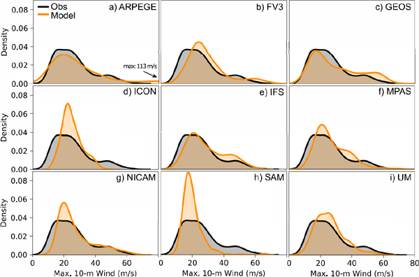
The observed v_max distribution has a broad primary peak centered near 20 m s⁻¹, a secondary peak near 50 m s⁻¹, and a fat tail toward higher values (Fig. 4). All models were able to produce this bi-modal distribution to some degree, but certain models deviated more from the observations than others. ICON and SAM deviated most dramatically: Both models produced a narrow primary peak, mainly because they were not able to simulate high intensities (Figs. 4d, h). FV3 and GEOS shifted the secondary peak to higher values (Figs. 4b, c), whereas IFS and MPAS shifted it to lower values (Figs. 4e, f). ARPEGE produced a very broad distribution, partly related to its over-intensification issue (Fig. 4a). NICAM reproduced the observed distribution for v_max > 25 m s⁻¹ better than the other models, but missed some of the weaker intensities with v_max < 20 m s⁻¹ (Fig. 4g).

The observed p_min distribution has a well-defined primary peak around 1000 hPa, and a fat tail extending toward lower pressures with a hint of a secondary maximum near 950 hPa (Fig. 5). All models captured the general shape of the observed distribution, with MPAS and UM matching the observations best (Figs. 5f, i). Most of the other models produced storms that were too deep, although in different ways. In FV3, the distribution had the same shape as the observation but shifted to deeper values (Figs. 5b); in IFS, the secondary maximum was much more pronounced than in the observations (Figs. 5f); and GEOS was somewhere between FV3 and IFS (Figs. 5c). In ARPEGE and NICAM, some storms were much deeper than the observations, causing the tail to stretch too far to the left (Figs. 5a, g). SAM is unique in that the main peak was shifted to much higher values. We shall note here that SAM's p_min values are ambiguous, because SAM uses the anelastic equations and pressure can only be determined to within a function proportional to the base-state density field with arbitrary amplitude (Bannon et al. 2006).

Lastly, we evaluated the overall TC activity by means of accumulated cyclone energy (ACE), a quantity that estimates the wind energy produced by one or multiple TCs over their lifetime. It is computed according to ACE = 10⁻⁴ , where v_max is in units of knots (1 knot = 0.51 m s⁻¹). In the context of this study, “ACE” refers to the combined ACE of all storms during the DYAMOND period. Concretely, for each model and the observations, we squared all 6-hourly v_max values, summed them up, and multiplied them by 10⁻⁴. According to the observations, the ACE during the DYAMOND period was 169 (Fig. 6). Since the wind speed enters the ACE calculation as a squared value, ACE is quite sensitive to uncertainty in the analyzed v_max values. We therefore estimated a lower and upper bound by assuming that all observed v_max records have an error of ±5 m s⁻¹, an estimate based on Torn and Snyder (2012) and Landsea and Franklin (2013). This assumption yielded a lower bound of 118 ACE units and an upper bound of 230 ACE units. Most models were within or slightly above these uncertainty bounds, indicating that the DYAMOND models produced realistic amounts of ACE, even without tuning. Only three models were clearly outside the uncertainty bounds: GEOS overestimated ACE, whereas ICON and SAM produced less ACE than observed.

Fig. 6.

Accumulated cyclone energy (ACE) from observations (grey) and models (orange). The lower bound of the uncertainty range in observed ACE assumes that all v_vmax observations have an error of −5 m s⁻¹ or +5 m s⁻¹ (upper bound). The arrows with numbers 2 and 3 along the UM bar mark the ACE in the two additional members of the UM mini-ensemble.

The three members of the UM mini-ensemble offer a glimpse at the intra-model spread. It seems that the intra-model spread is in the range of the observational uncertainty, but slightly less than the inter-model spread (as far as the limited numbers of ensemble members can tell).

Finally, we emphasize that none of the DYAMOND models featured ocean coupling. Consequently, the simulations did not account for the effect of storm-generated ocean cold wakes—which is to induce some weakening. In an otherwise unbiased model, TC intensity should therefore be somewhat higher than observed; in other words, the models that reproduce the observed TC intensities/ACE may actually under-estimate TC intensity/ACE.

3.3 Tropical cyclone size

Size is an important TC parameter because it correlates with the risk for storm surge, but it is infrequently used for model validations. We examined the radius of gale-force winds (r₁₇) and here present the median of all r₁₇ records as our metric of choice (Fig. 7). Results for r₂₅ and r₃₂ were qualitatively similar (not shown), indicating that the results are not sensitive to a particular wind speed threshold. The observational error bars were computed by increasing/decreasing each r₁₇ record by 50 % before determining the median value (Landsea and Franklin 2013).

Fig. 7.

Average storm size as measured by the median 17 m s⁻¹ wind radius for each storm quadrant from observations (black) and models (orange). Dashed grey circles indicate radius intervals of 100 km. The error bars in the observations are based on an error estimate of 50 %.

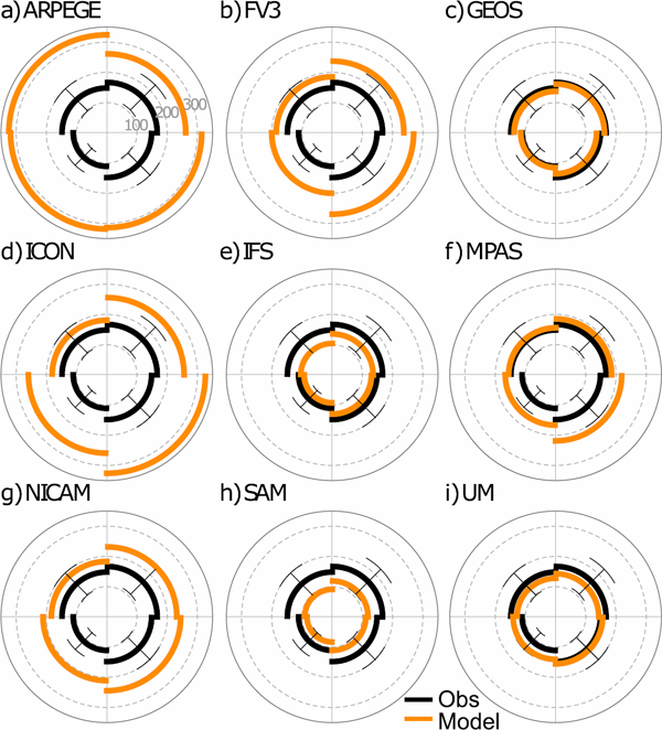
In general, the models overestimated TC size. TCs in ARPEGE, FV3, ICON, and NICAM were substantially larger than observed (Figs. 7a, b, d, g). In fact, ARPEGE and ICON produced very expansive wind fields, and their median r₁₇ reached radially outward to 300 km (more than double the observations). In contrast, the median size of TCs in GEOS matched the observations remarkably well (Fig. 7c), and UM came in as a clear second (Fig. 7i). Storms in IFS and SAM were somewhat smaller than observed, but still within the uncertainty estimates (Figs. 7e, h). A common bias in the models was associated with the asymmetry of the wind field. Concretely, the observed median r₁₇ was largest in the northeast quadrant, but in FV3, ICON, MPAS, and NICAM, it was largest in the southeast quadrant (Figs. 7b, d, f, g). This result suggests that the models are deficient in their representation of TC structure, the prospect of which is examined in the next section.

3.4 Tropical cyclone structure

The TC wind-pressure relationship, i.e., the function that relates p_min to v_max, is often used to inform whether models simulate TC structure realistically. The DYAMOND models produced a variety of wind pressure relationships, with some models being closer to the observation than others (Fig. 8). FV3 and GEOS stand out for reproducing the observed relationship remarkably well (Figs. 8b, c). Most other models have a tendency to produce a relationship that drops off too fast, or in other words, for a given p_min, the v_max is too low. This behavior was most pronounced in ICON (Fig. 8d), and less noticeable in ARPEGE and MPAS (Figs. 8a, f). A possible explanation for this behavior is discussed in Section 4. SAM was unique and had an unrealistic wind-pressure relationship that bended upward (Fig. 8h). This phenomenon was not due to a single outlier but likely related to the surface pressure field being an ambiguous quantity in this model (see also Section 3.2).

Fig. 8.

TC wind-pressure relationships from observations (black) and models (orange). The curves are least-squares fitted quadratic functions. Note: the peculiar shape of the fit line in SAM (h) is not caused by the obvious outlier at 65 m s⁻¹ and 950 hPa. Excluding this outlier will not change the fit substantially.

Since the 10-m winds in a TC and therefore v_max are strongly affected by the surface layer parameterization, we also investigated the relationship between p_min and 850-hPa v_max. The graphs were qualitatively similar to Fig. 8 (not shown), indicating that the wind-pressure relationships in Fig. 8 are not merely a product of each model's boundary layer and surface layer parameterizations, but they stem from differences in the overall model implementation including the dynamical cores.

Snapshots of 10-m wind speed demonstrate the diversity of the models in simulating the surface wind field (Fig. 9). There were striking differences in eyewall shape, size, and symmetry, as well as in the radial extent of the wind field. Some models produced unrealistic wind fields, either too large and too strong (ARPEGE; Fig. 9a), or too faint and with peculiar waviness (SAM; Fig. 9h). The wind fields of FV3, GEOS, and MPAS were arguably most similar to that of a canonical intense TC, with a distinct eyewall that contained multiple convective- and mesoscale asymmetries (Figs. 9b, c, f).

Fig. 9.

Snapshots of 10-m wind speed of the strongest storm from each model at the time of peak intensity.

The ICON example was unique in that it did not reveal a distinct eyewall with sharp gradients; its wind field was rather diffuse and spread out over a large area (Fig. 9d). In contrast, the IFS example was a very small TC with a radially constrained wind field (Fig. 9e). The NICAM example, Fig. 9g, had an even larger hurricane-force (wind speed ≥ 33 m s⁻¹) wind field than ICON, but it also had a distinct eyewall like most other models—albeit somewhat smoother than the eyewalls in FV3, GEOS, and MPAS. The wind field from the UM example exhibited the smoothest structure, the widest eyewall, and the clearest imprint of the model mesh—all consistent with UM being the model with the lowest resolution (Fig. 9i).

A closer look at the kinematic and thermodynamic structure of the simulated TCs was made possible by creation of composite means of the azimuthally-averaged tangential wind, vertical wind, boundary layer inflow, and temperature anomaly (Figs. 10–12). Each composite mean comprised all instances (“snapshots”) where a storm's v_max is ≥ 33 m s⁻¹. This means that each panel reflects the aggregate information from 10–100 s of individual snapshots (as noted in Fig. 10), a number that should be large enough to obtain at least a somewhat robust analysis, even if the number of TCs is limited. The data of the composite means are available for download (Judt et al. 2020).

Fig. 10.

Composite means of azimuthally-averaged tangential wind speed (grey shading) and radial/vertical flow (colored streamlines) from each model in radius-height space. The 20 m s⁻¹-contour is annotated for reference. The composite means were created by averaging over all instances (“snapshots”) where a storm's v_max ≥ 33 m s⁻¹. The number of individual snapshots comprising each composite is indicated next to the model name.

Fig. 11.

Composite means of azimuthally-averaged radial wind speed in the lowest 2 km from each model in radius-height space. The dashed black line depicts the inflow layer height, here defined as the layer with radial wind < −1 m s⁻¹. The composite means were created by averaging over all instances (“snapshots”) where a storm's v_max ≥ 33 m s⁻¹.

Fig. 12.

Composite means of the TC warm core from each model, computed as the azimuthally-averaged temperature anomaly with respect to the mean temperature between r = 300–700 km. The composite means were created by averaging over all instances (“snapshots”) where a storm's v_max ≥ 33 m s⁻¹.

Broadly speaking, all models produced a typical kinematic structure, that is, a well-defined primary circulation with a tangential wind maximum in the lower troposphere near the storm center and a well-defined secondary circulation manifested by strong radial inflow in the boundary layer, rising motion in the eyewall region, and radial outflow in the middle to upper troposphere (Fig. 10). Despite the overall agreement, there were noteworthy differences between the models, which will be discussed in the next few paragraphs.

The differences in the overall tangential wind structure can be elucidated by comparing the size of the radius of maximum tangential wind, the compactness of the wind maximum (specifically, the radial extent of the 35 m s⁻¹ isotach), and the decay of the tangential wind in the radial and vertical direction. The composite storms had radii of maximum tangential wind roughly between 30 km and 70 km, with ARPEGE and IFS on the lower end (Figs. 10a, e) and ICON on the upper end (Fig. 10d). In FV3 and MPAS, the wind maximum was comparatively narrow and confined, and the radial extent of the 35 m s⁻¹ isotach was less than 20 km (Figs. 10b, f). Contrarily, in ICON and NICAM, the wind maximum was rather broad, and the radial extent of the 35 m s⁻¹ isotach was greater than 50 km (Figs. 10d, g). Differences in the radial and vertical decay rates mirror the previous discussion of storm size, that is, models in which the tangential wind decayed more slowly, such as in ICON and NICAM, were the ones that produced comparatively larger storms. Given the lack of an equivalent observational dataset, it is difficult to assess which model produced a particularly realistic tangential wind structure. The observational composites of Gao et al. (2019, their Fig. 5c) and Komaromi and Doyle (2017, their Fig. 7a) at least suggest that no model produced a particularly unrealistic structure.

As for the vertical motion, ARPEGE and IFS had the steepest eyewall slopes (Figs. 10a, e). The other extreme was UM, which had the most pronounced eyewall tilt (Fig. 10i). In ICON and NICAM, the eyewall updraft was spread out and diffuse (Figs. 10d, g), but in IFS and MPAS it was relatively narrow and confined (Figs. 10e, f). Besides these differences in the eyewall region, there were other differences in the rainband region. Specifically, the vertical motion between r = 100 and r = 250 km was noticeably stronger in ICON, MPAS, and NICAM than in GEOS, IFS, and SAM (Figs. 10d, f, g versus Figs. 10c, e, h). This difference may be a reflection of more or stronger rainbands in the former models.

Again, it is difficult to say which models produced a particularly realistic structure because no equivalent observational dataset exists for the TCs observed during the DYAMOND period. Stern and Nolan (2009) demonstrated that the slope of the eyewall depends on the size of the radius of maximum wind, which would explain why the eyewall updraft in IFS had a steeper slope than in UM. However, The Stern and Nolan study cannot explain the differences between models with similarly sized radii of maximum wind, such as MPAS and UM.

The upper-tropospheric outflow also differed between the models, especially with regard to the altitude of the outflow maximum and the depth of the outflow layer. For instance, the outflow was comparatively deep in FV3 (Fig. 10b) and comparatively shallow in IFS (Fig. 10e). In ARPEGE and ICON, the outflow maximum occurred at a height of 15 km (Figs. 10a, d), but in most of the other models, it occurred mostly below 15 km.

One particularly noteworthy feature, produced somewhat more prominently by FV3, GEOS, and IFS, is the descending flow above the outflow layer that merges with the ascending outflow from below (Figs. 10b, c, e). We are not aware of either observational or modeling studies that demonstrate such a feature in TCs; on the contrary, there is reasonable evidence to suggest that at least in intense TCs, it may be common to have a shallow layer of weak inflow atop the upper-level outflow layer (e.g., Kieu et al. 2016; Komaromi and Doyle 2017; Heng et al. 2017; Duran and Molinari 2018).

Inter-model differences in the boundary layer inflow were mostly in the form of variations of inflow layer depth and strength (Fig. 11). Specifically, IFS and SAM produced comparatively shallow inflow layers that did not extend much above 1 km height (Figs. 11e, h). In GEOS and ICON, the inflow layer had a maximum depth of 1.5 km (Figs. 11c, d), and in the other models, its maximum depth extended slightly above 1.5 km. The observational composite of Zhang et al. (2011, their Fig. 5b) indicates that the inflow layer depth increases from 900 m at the radius of maximum wind to 1.5 km roughly 200 km from the center, which is in broad agreement with most of the models.

From basic TC dynamics, one would expect that the inflow strength correlates with the average intensity of the TCs simulated by the models. However, this was not the case. For example, ICON, which simulated mostly weak TCs, produced stronger inflow than FV3, MPAS, and NICAM, which simulated much stronger TCs (Fig. 11d vs. Figs. 11b, f, g). In fact, with inflow magnitudes of 9 m s⁻¹, the inflow in FV3, MPAS, and NICAM was relatively weak, compared not only to the other models, but also to observations, which show an inflow magnitude of 20 m s⁻¹ (Zhang et al. 2011).

Besides the kinematic structure, we also explored the thermodynamic TC structure in our set of global storm-resolving simulations. To this end, we examined the TC warm core, here represented by the temperature anomaly with respect to the mean temperature between r = 300 km and 700 km (Fig. 12). All models produced a warm core and agreed on the general core structure (expansive in the upper levels, radially confined below). Differences emerged mostly in the vertical structure of the warming inside the TC eye, and in the upper and lower level temperature anomalies outside the eye.

Most models agreed that the warm anomaly peaks at a height of just less than 10 km. More pronounced differences between the models appeared in the vertical structure of the warm core, which ranged from a single, vertically confined maximum in FV3 and GEOS (Figs. 12b, c), to an extended vertical column in NICAM (Fig. 12g), to a clear double maximum of anomalously warm air in UM (Fig. 12i). The other models fell somewhere among these three distinct cases. Most observational studies indicate that the warm core is maximized in the upper troposphere (Frank 1977; Brammer and Thorncroft 2017; Komaromi and Doyle 2017), in agreement with most of the DYAMOND models. However, Stern and Nolan (2012) claimed that the maximum warming should be between 4 km and 8 km, with a potential secondary maximum at higher altitudes. Kieu et al. (2016) also claimed that a double-warm core structure is the norm rather than the exception. If one were to believe the Stern and Nolan and Kieu et al. studies, then UM had a particularly realistic thermodynamic structure, even though it was an outlier among the DYAMOND models.

Compared to the model differences in terms of the warm core, the differences above the outflow layer were equally if not more striking. Above 15-km height, the models did not even agree on the sign of the temperature anomaly. In particular, IFS and ARPEGE produced a strong cool anomaly (< −3 K; incidentally, IFS and ARPEGE were the only spectral models), whereas NICAM, SAM, and UM produced a warm anomaly. FV3, GEOS, ICON, and MPAS were somewhere between the extremes and produced a weak cool anomaly (> −1 K). Observational composites generally show a weak cold anomaly above the outflow layer (Frank 1977; Komaromi and Doyle 2017), although instantaneous snapshots of intense TCs may also show strong cold anomalies (Komaromi and Doyle 2017).

Temperature differences were also found in the boundary layer, although less dramatic: NICAM was anomalously cool (Fig. 12g), and IFS was anomalously warm (Fig. 12e). The other models had weak cool anomalies or no clear signal. Note that IFS and NICAM were polar opposites of each other (NICAM: warm in the upper levels, cool in the lower levels; IFS: vice versa).

3.5 Sensitivity of tropical cyclone formation and intensity to model resolution and parameterized deep convection

In addition to the primary high-resolution simulation, some DYAMOND models produced sensitivity runs with lower resolution. For example, ICON produced six simulations with mesh spacings of 2.5, 5, 10, 20, 40, and 80 km, all without parameterized convection (hereafter referred to as ICON no-conv), and an additional three simulations with mesh spacings of 20, 40, and 80 km with parameterized convection (ICON conv). These nine simulations provided an opportunity to investigate the sensitivity to model resolution and parameterized convection in a controlled manner (Figs. 13, 14) .

Fig. 13.

TC tracks and numbers from various ICON runs (orange) and observations (grey). Left: ICON runs without deep convective parameterization, right: ICON runs with deep convective parameterization. The model resolution, given in each panel, decreases from top to bottom.

Fig. 14.

ACE from observations (grey) and various ICON runs with (light orange) or without (dark orange) deep convective parameterization. Model resolution decreases from top to bottom. The error bars are the lower an upper bounds assuming that all v_vmax observations have an error of ± 5 m s⁻¹.

As for sensitivity to resolution, there was a clear inverse relationship, as the number of simulated TCs increased when resolution was decreased (Fig. 13, left column). Concretely, the highest resolution run produced the fewest TCs (15; Fig. 13a), and the lowest resolution run produced the most TCs (50; Fig. 13h). In the simulations with intermediate resolution, the number of TCs was relatively constant (around 20). The sensitivity to resolution seemed to be basin dependent. Specifically, in the Atlantic and Eastern Pacific, the 80-km ICON produced five to six times as many TCs as the 2.5-km ICON (Figs. 13a, h), but in the Western Pacific, the 80-km ICON produced only two times as many TCs as the 2.5-km ICON. As a consequence, the fractional ratio of storm numbers among the ocean basins relative to the global total number was much better in the higher resolution runs than in the lower resolution runs. In the Indian Ocean, the number of events seemed to be insensitive to resolution, and each run produced either one or two TCs.

As for sensitivity to parameterized convection, the model produced dramatically fewer TCs once the parameterization was turned on (Fig. 13, left vs. right column). This effect was most pronounced at lower resolution. Specifically, the number of TCs dropped from 23 to 17 in the 20-km runs (Figs. 13d, e), from 21 to 14 in the 40-km runs (Figs. 13f, g), and from 50 to a mere 9 in the 80-km runs (Figs. 13h, i).

The runs with parameterized convection also featured substantially lower ACE (Fig. 14). Again, the effect was most dramatic at lower resolution, but even for an intermediate resolution of 20 km, the ACE was reduced by 65 %. In fact, at least for the 20-km runs, the reduction in ACE is more dramatic than the reduction in TC number, which suggests that convection parameterization not only reduces the number of TCs but also makes TCs weaker and/or shortens their lifetime.

Notably, the ICON no-conv runs produced more or less the same amount of ACE at all resolutions (Fig. 14). Evidently, the lack of intense storms in the lower-resolution runs was compensated by a larger number of weak storms. An interesting follow-up question would be whether this compensation was pure luck or whether the amount of background available potential energy that is converted into kinetic energy by TCs is resolution-independent, such as mean precipitation (Hohenegger et al. 2020).

4. Discussion

One of the drawbacks of global storm-resolving models is their immense computational cost, which results in questions about cost versus benefit. One may, for example, postulate that regional high-resolution models suffice for TC prediction. Although a practical alternative, regional models have disadvantages such as determining the ideal domain size and placement for a regional domain. More importantly, regional domains require lateral boundary conditions, which have “serious negative effects” (Warner et al. 1997). One of those effects is that errors creep in through the boundaries and render longer-range forecasts less accurate than those made by global models. In other words, regional models are very dependent on the global model forcing being “good enough”.

One may also follow Manganello et al. (2012) and argue that hydrostatic models with mesh spacings of 10 km and parameterized convection are sufficient for producing realistic TCs. Nonetheless, mesh spacings < 5 km are still required for realistically simulating v_max and the dynamic processes in the TC inner core (e.g., Chen et al. 2007; Gentry and Lackmann 2010; Judt and Chen 2010; Gopalakrishnan et al. 2012; Davis 2018). Observations and numerical models indicate that such processes are important for rapid intensification (e.g., Miyamoto and Takemi 2015; Guimond et al. 2016; Judt and Chen 2016). In fact, a case study by Fox and Judt (2018) suggested that simulating extreme cases of rapid intensification requires a horizontal grid spacing ≤ 1 km. Since extreme storms are highly disruptive to society, being able to reliably predict or project intense TCs has great value.

As a potential easy target for bias reduction in the models, we examined whether models with similar biases used similar parameterization schemes. For example, we investigated whether the models with a TKE-like boundary layer parameterization produced similar intensity biases versus models that used a diagnostic eddy diffusivity. However, no such relationships were found. In the end, there are variety of reasons for the model diversity, including but not limited to: cloud microphysics, boundary layer processes, and the dynamical cores (with differences in effective resolution).

In agreement with other studies, this paper also demonstrates that high resolution is necessary yet not sufficient for capturing the v_max of TCs. For example, ICON was tied with ARPEGE for highest resolution (2.5 km), yet ICON struggled to produce intense TCs while ARPEGE produced unrealistically strong TCs. These intensity biases are likely a consequence of the respective model's surface flux formulation, as demonstrated by Fig. 15, which illustrates the surface fluxes of momentum and latent heat over a 300 × 300 km area centered on the strongest TC in each model. The drag in ICON increased much faster with wind speed than that in ARPEGE (Fig. 15a), which means that there was a comparatively stronger “break” on the surface wind in ICON. ICON also had significantly weaker latent heat fluxes for a given wind speed, providing less “fuel” (Fig. 15b).

Fig. 15.

Momentum flux (top) and latent heat flux (bottom) from ARPEGE (black) and ICON (blue) as a function of wind speed. The data are from the same time and domain as the snapshots in Fig. 9. Instead of a raw scatter plot, the data are binned and the color saturation is a measure of data points per bin (N) as indicated by the colorbars.

The monotonically increasing momentum flux in Fig. 15a also indicates that the models did not account for the saturation of the drag at wind speeds above 25 m s⁻¹ (e.g., Powell et al. 2003; Donelan 2004; Chen et al. 2013; Curcic and Haus 2020). This shortcoming was also found in other models (not shown), and it may be the reason why the wind–pressure relationship in several models deviated from observations at higher winds (Fig. 8). In fact, the wind–pressure relationship in IFS seems to improve when drag is computed in a more realistic three-way coupled atmosphere–wave–ocean model (Magnusson et al. 2019).

One implicit assumption underlying this study is that the differences in TC characteristics between models are due to differences in model formulation. Strictly speaking, this assumption is only valid if the models simulate the same TCs or if the number of TC samples is large enough to produce a realistic TC climatology; neither condition is met here. Therefore, some of the inter-model differences, such as the differences in TC structure revealed by Figs. 9–12, are due in part to limited sampling. Unfortunately, addressing this shortcoming by extending the simulations is not practical, mainly for the unwieldy computational cost and storage requirements. Furthermore, it is difficult to say exactly what number of samples would be enough to render sampling errors insignificant. We acknowledge the weaknesses introduced by sampling limitation but argue that the analyses presented in this paper are nonetheless insightful for a model intercomparison.

Lastly, there is much evidence that the storm count (and storm-count-related model biases) are sensitive to the tracker (Roberts et al. 2020; Vannière et al. 2020). This can be an issue when models are compared because weak TCs might be over- or under-detected depending on the threshold used. We estimated this sensitivity by changing the minimum v_max threshold in the quality-control process. Specifically, we computed ACE and storm count after increasing the minimum v_max requirement from 7.5 m s⁻¹ to 15 m s⁻¹ and then to 32 m s⁻¹. In other words, we first considered all TCs, then only TCs of at least tropical storm intensity, and finally only TCs of hurricane/typhoon intensity. It turns out that ACE is insensitive to these changes in the v_max threshold, presumably because ACE is dominated by intense storms that are accounted for under all three thresholds. By contrast, the storm count does show sensitivity, and the number of TCs drops when the threshold is increased from 15 to 32 m s⁻¹. This drop is more pronounced for the observations than for the simulations; consequently, models that produced the right number of TCs under the 7.5 m s⁻¹ threshold produced too many TCs under the 32 m s⁻¹ threshold. For example, GEOS produced 24 TCs under the 7.5 m s⁻¹ threshold, the same number as observed. Under the 32 m s⁻¹ threshold, GEOS produced 17 TCs, which is 7 less than that in the observations. In the end, the sensitivity to thresholds in the tracking process indicates that storm count, although often used and intuitive, is a sub-optimal metric for evaluating numerical models, and insensitive metrics such as ACE are better suited for this purpose.

5. Summary and conclusions

We evaluated nine global storm-resolving models that participated in the DYAMOND initiative (Stevens et al. 2019) in their ability to simulate TCs. Specifically, we validated and compared the number of TCs each model produced, and the tracks, intensity, size, and structure of the TCs. With mesh spacings between 2.5 km and 7.8 km, the DYAMOND models are the highest-resolution global models that have thus far been analyzed for this purpose.

The results indicate that global storm-resolving models produce realistic TCs and remove longstanding biases known from previous generations of global models, such as the difficulty to capture TC intensity. However, TCs are strongly affected by model formulation, and essentially all models had biases.

We found that no model did best in all regards, although some models did, generally speaking, better than others. For instance, GEOS reproduced the observed number of TCs³, captured TC size better than any other model, and produced a realistic wind-pressure relationship. However, GEOS also produced too many strong storms and had the highest ACE bias of all models (it is unclear if ocean coupling would reduce this bias). Other models that did generally well were FV3, MPAS, and UM. On the other hand, ICON, IFS, and SAM had some issues with size, structure, and intensity. For example, ICON and SAM produced storms that were too weak. ICON, IFS, and SAM also could not capture the wind–pressure relationship as realistically as GEOS, FV3, and MPAS; this points to deficiencies in the numerical formulations of the former models.

We also found that parameterized convection in the ICON model strongly reduces the number and intensity of TCs in comparison to simulations without convection parameterization (at least for simulations with a mesh spacing > 20 km). This sensitivity highlights problems and ambiguities that come with parameterizing deep convection.

In a nutshell, we believe that the ability to realistically simulate TCs in global models is critical for weather and climate prediction. This study demonstrates that global-storm resolving models are an optimal tool to advance TC prediction; however, these models should be improved to unleash their full potential. One such avenue for improvement is to update the boundary and surface layer parameterizations based on results from current research.

Acknowledgments

This material is based upon work supported by the National Center for Atmospheric Research, which is a major facility sponsored by the National Science Foundation under Cooperative Agreement no. 1852977. Support by the Centre of Excellence ESiWACE is acknowledged. ESiWACE has received funding from the European Union's Horizon 2020 research and innovation programme under grant agreement numbers 675191 and 823988. The authors thank the German Climate Computing Center for hosting, providing access to and supporting the evaluation of the DYAMOND data sets. We acknowledge high-performance computing support from Cheyenne (doi:10.5065/D6RX99HX) provided by NCAR's Computational and Information Systems Laboratory, sponsored by the National Science Foundation. RS, MS, MN and CK were supported by the FLAGSHIP2020 within the priority study 4 (Advancement of meteorological and global environmental predictions utilizing observational “Big Data”) and the Integrated Research Program for Advancing Climate Models (TOUGOU) grant number JPMXD0717935457 from the Ministry of Education, Culture, Sports, Science, and Technology of Japan. The NICAM simulation was performed on the Earth Simulator of the Japan Agency for Marine-Earth Science and Technology. MR, PLV, and BV acknowledge funding from the EU H2020 PRIMAVERA project under grant agreement no. 641727. MK was supported by the NSF Grant AGS1418309 to Stony Brook University, and by the NCAR-Wyoming Supercomputing Center, where the SAM simulation was performed. The authors would also like to thank David Ahijvevych for his assistance with the GFDL tracker, and Daniel Stern, William Komaromi, and Kevin Hodges for valuable comments. The comments from two anonymous reviewers and three editorial members of this journal also helped in improving the manuscript.

Footnotes

¹ Global storm-resolving models are also referred to as global cloud-resolving models or global convection-permitting models. No matter what name one prefers, the important aspect of these models is that they explicitly simulate convective storms and how smaller scales of motions couple to large-scale circulation systems.

² The IFS model considered here is an experimental version of the operational IFS model with 4-km mesh spacing and explicitly simulated deep convection.

³ This result is conditional and only valid when using the 7.5 m s⁻¹ minimum v_max threshold for TC tracking.

References

•  Bannon,  P. R.,  J. M.  Chagnon, and  R. P.  James, 2006: Mass conservation and the anelastic approximation. Mon. Wea. Rev., 134, 2989-3005.
•  Bengtsson,  L.,  K. I.  Hodges,  M.  Esch,  N.  Keenlyside,  L.  Kornblueh,  J.-J.  Luo, and  T.  Yamagata, 2007: How may tropical cyclones change in a warmer climate? Tellus A, 59, 539-561.
•  Biswas,  M. K.,  D.  Stark, and  L.  Carson, 2018: GFDL Vortex Tracker Users Guide Version 3.9a. National Center for Atmospheric Research, Developmental Testbed Center, 35 pp. [Available at https://dtcenter.org/sites/default/files/community-code/gfdl/standalone_tracker_UG_v3.9a.pdf.]
•  Brammer,  A., and  C. D.  Thorncroft, 2017: Evaluation of reanalysis tropical cyclone structure with global hawk 1 dropsonde observations. 29 pp. [Available at http://www.atmos.albany.edu/facstaff/chris/nasa2017/Brammer-Thorncroft2017b.pdf.]
•  Bubnová,  R.,  G.  Hello,  P.  Bénard, and  J.-F.  Geleyn, 1995: Integration of the fully elastic equations cast in the hydrostatic pressure terrain-following coordinate in the framework of the ARPEGE/Aladin NWP system. Mon. Wea. Rev., 123, 515-535.
•  Camargo,  S. J.,  A. G.  Barnston, and  S. E.  Zebiak, 2005: A statistical assessment of tropical cyclone activity in atmospheric general circulation models. Tellus A, 57, 589-604.
•  Chen,  S. S.,  J. F.  Price,  W.  Zhao,  M. A.  Donelan, and  E. J.  Walsh, 2007: The CBLAST-hurricane program and the next-generation fully coupled atmosphere–wave–ocean models for hurricane research and prediction. Bull. Amer. Meteor. Soc., 88, 311-318.
•  Chen,  S. S.,  W.  Zhao,  M. A.  Donelan, and  H. L.  Tolman, 2013: Directional wind-wave coupling in fully coupled atmosphere-wave-ocean models: Results from CBLAST-hurricane. J. Atmos. Sci., 70, 3198-3215.
•  Curcic,  M., and  B. K.  Haus, 2020: Revised estimates of ocean surface drag in strong winds. Geophys. Res. Lett., 47, e2020GL087647, doi:10.1029/2020GL087647.
•  Davis,  C. A., 2018: Resolving tropical cyclone intensity in models. Geophys. Res. Lett., 45, 2082-2087.
•  Davis,  C.,  W.  Wang,  S. S.  Chen,  Y.  Chen,  K.  Corbosiero,  M.  DeMaria,  J.  Dudhia,  G.  Holland,  J.  Klemp,  J.  Michalakes,  H.  Reeves,  R.  Rotunno,  C.  Snyder, and  Q.  Xiao, 2008: Prediction of landfalling hurricanes with the advanced hurricane WRF model. Mon. Wea. Rev., 136, 1990-2005.
•  DeMaria,  M.,  C. R.  Sampson,  J. A.  Knaff, and  K. D.  Musgrave, 2014: Is tropical cyclone intensity guidance improving? Bull. Amer. Meteor. Soc., 95, 387-398.
•  Donelan,  M. A.,  B. K.  Haus,  N.  Reul,  W. J.  Plant,  M.  Stiassnie,  H. C.  Graber,  O. B.  Brown, and  E. S.  Saltzman, 2004: On the limiting aerodynamic roughness of the ocean in very strong winds. Geophys. Res. Lett., 31, L18306, doi:10.1029/2004GL019460.
•  Duran,  P., and  J.  Molinari, 2018: Dramatic inner-core tropopause variability during the rapid intensification of Hurricane Patricia (2015). Mon. Wea. Rev., 146, 119-134.
•  Fox,  K. R., and  F.  Judt, 2018: A numerical study on the extreme intensification of Hurricane Patricia (2015). Wea. Forecasting, 33, 989-999.
•  Frank,  W. M., 1977: The structure and energetics of the tropical cyclone. I. Storm structure. Mon. Wea. Rev., 105, 1119-1135.
•  Fudeyasu,  H.,  Y.  Wang,  M.  Satoh,  T.  Nasuno,  H.  Miura, and  W.  Yanase, 2008: Global cloud-system-resolving model NICAM successfully simulated the lifecycles of two real tropical cyclones. Geophys. Res. Lett., 35, L22808, doi:10.1029/2008GL036003.
•  Gao,  K.,  L.  Harris,  J.-H.  Chen,  S.-J.  Lin, and  A.  Hazelton, 2019: Improving AGCM hurricane structure with twoway nesting. J. Adv. Model. Earth Syst., 11, 278-292.
•  Gentry,  M. S., and  G. M.  Lackmann, 2010: Sensitivity of simulated tropical cyclone structure and intensity to horizontal resolution. Mon. Wea. Rev., 138, 688-704.
•  Gopalakrishnan,  S. G.,  S.  Goldenberg,  T.  Quirino,  X.  Zhang,  F.  Marks, Jr.,  K.-S.  Yeh,  R.  Atlas, and  V.  Tallapragada, 2012: Toward improving high-resolution numerical hurricane forecasting: Influence of model horizontal grid resolution, initialization, and physics. Wea. Forecasting, 27, 647-666.
•  Green,  B. W., and  F.  Zhang, 2013: Impacts of air-sea flux parameterizations on the intensity and structure of tropical cyclones. Mon. Wea. Rev., 141, 2308-2324.
•  Guimond,  S. R.,  G. M.  Heymsfield,  P. D.  Reasor, and  A. C.  Didlake, Jr., 2016: The rapid intensification of Hurricane Karl (2010): New remote sensing observations of convective bursts from the Global Hawk platform. J. Atmos. Sci., 73, 3617-3639.
•  Hamill,  T. M.,  J. S.  Whitaker,  M.  Fiorino, and  S. G.  Benjamin, 2011: Global ensemble predictions of 2009's tropical cyclones initialized with an ensemble Kalman filter. Mon. Wea. Rev., 139, 668-688.
•  Harper,  B. A.,  J. D.  Kepert, and  J. D.  Ginger, 2010: Guidelines for converting between various wind averaging periods in tropical cyclone conditions. WMO/TD-No. 1555. World Meteorological Organization. 54 pp. [Available at https://library.wmo.int/doc_num.php?explnum_id=290.]
•  Heng,  J.,  Y.  Wang, and  W.  Zhou, 2017: Revisiting the balanced and unbalanced aspects of tropical cyclone intensification. J. Atmos. Sci., 74, 2575-2591.
•  Hodges,  K. I., and  N. P.  Klingaman, 2019: Prediction errors of tropical cyclones in the western North Pacific in the Met Office global forecast model. Wea. Forecasting, 34, 1189-1209.
•  Hohenegger,  C.,  L.  Kornblueh,  D.  Klocke,  T.  Becker,  G.  Cioni,  J. F.  Engels,  U.  Schulzweida, and  B.  Stevens, 2020: Climate statistics in global simulations of the atmosphere, from 80 to 2.5 km grid spacing. J. Meteor. Soc. Japan, 98, 73-91.
•  Judt,  F., and  S. S.  Chen, 2010: Convectively generated potential vorticity in rainbands and formation of the secondary eyewall in Hurricane Rita of 2005. J. Atmos. Sci., 67, 3581-3599.
•  Judt,  F., and  S. S.  Chen, 2016: Predictability and dynamics of tropical cyclone rapid intensification deduced from high-resolution stochastic ensembles. Mon. Wea. Rev., 144, 4395-4420.
•  Judt,  F.,  D.  Klocke,  R.  Rios-Berrios,  B.  Vanniere, and  F.  Ziemen, 2020: Tropical cyclones in global storm-resolving models. Version 1.0. UCAR/NCAR -DASH Repository. doi:10.5065/5pfk-sm48.
•  Kanada,  S.,  A.  Wada,  M.  Nakano, and  T.  Kato, 2012: Effect of planetary boundary layer schemes on the development of intense tropical cyclones using a cloud-resolving model. J. Geophys. Res., 117, D03107, doi: 10.1029/2011JD016582.
•  Kepert,  J. D., 2012: Choosing a boundary layer parameterization for tropical cyclone modeling. Mon. Wea. Rev., 140, 1427-1445.
•  Khairoutdinov,  M. F., and  D. A.  Randall, 2003: Cloud resolving modeling of the ARM summer 1997 IOP: Model formulation, results, uncertainties, and sensitivities. J. Atmos. Sci., 60, 607-625.
•  Kieu,  C.,  V.  Tallapragada,  D.-L.  Zhang, and  Z.  Moon, 2016: On the development of double warm-core structures in intense tropical cyclones. J. Atmos. Sci., 73, 4487-4506.
•  Knapp,  K. R.,  M. C.  Kruk,  D. H.  Levinson,  H. J.  Diamond, and  C. J.  Neumann, 2010: The International Best Track Archive for Climate Stewardship (IBTrACS) Unifying tropical cyclone data. Bull. Amer. Meteor. Soc., 91, 363-376.
•  Knapp,  K. R.,  H. J.  Diamond,  J. P.  Kossin,  M. C.  Kruk, and  C. J.  Schreck, 2018: International Best Track Archive for Climate Stewardship (IBTrACS) Project, Version 4. NOAA/National Centers for Environmental Information, doi:10.25921/82ty-9e16.
•  Komaromi,  W. A., and  J. D.  Doyle, 2017: Tropical cyclone outflow and warm core structure as revealed by HS3 dropsonde data. Mon. Wea. Rev., 145, 1339-1359.
•  Landsea,  C. W., and  J. L.  Franklin, 2013: Atlantic hurricane database uncertainty and presentation of a new database format. Mon. Wea. Rev., 141, 3576-3592.
•  Lee,  C.-Y., and  S. S.  Chen, 2014: Stable boundary layer and its impact on tropical cyclone structure in a coupled atmosphere-ocean model. Mon. Wea. Rev., 142, 1927-1944.
•  Lin,  S.-J., 2004: A “vertically Lagrangian” finite-volume dynamical core for global models. Mon. Wea. Rev., 132, 2293-2307.
•  Magnusson,  L.,  J.-R.  Bidlot,  M.  Bonavita,  A. R.  Brown,  P. A.  Browne,  G.  De Chiara,  M.  Dahoui,  S. T. K.  Lang,  T.  McNally,  K. S.  Mogensen,  F.  Pappenberger,  F.  Prates,  F.  Rabier,  D. S.  Richardson,  F.  Vitart, and  S.  Malardel, 2019: ECMWF activities for improved hurricane forecasts. Bull. Amer. Meteor. Soc., 100, 445-458.
•  Malardel,  S.,  N.  Wedi,  W.  Deconinck,  M.  Diamantakis,  C.  Kuehnlein,  G.  Mozdzynski,  M.  Hamrud, and  P.  Smolarkiewicz, 2016: A new grid for the IFS. ECMWF Newsl., 146, 23-28.
•  Manganello,  J. V.,  K. I.  Hodges,  J. L.  Kinter III,  B. A.  Cash,  L.  Marx,  T.  Jung,  D.  Achuthavarier,  J. M.  Adams,  E. L.  Altshuler,  B.  Huang,  E. K.  Jin,  C.  Stan,  P.  Towers, and  N.  Wedi, 2012: Tropical cyclone climatology in a 10-km global atmospheric GCM: Toward weatherresolving climate modeling. J. Climate, 25, 3867-3893.
•  Marchok,  T. P., 2002: How the NCEP tropical cyclone tracker works. Proceedings of the 25th Conference on Hurricanes and Tropical Meteorology, San Diego, CA, P1.13, American Meteorological Society.
•  Miyamoto,  Y., and  T.  Takemi, 2015: A triggering mechanism for rapid intensification of tropical cyclones. J. Atmos. Sci., 72, 2666-2681.
•  Mogensen,  K. S.,  L.  Magnusson, and  J.-R.  Bidlot, 2017: Tropical cyclone sensitivity to ocean coupling in the ECMWF coupled model. J. Geophys. Res.: Oceans, 122, 4392-4412.
•  Nakano,  M.,  M.  Sawada,  T.  Nasuno, and  M.  Satoh, 2015: Intraseasonal variability and tropical cyclogenesis in the western North Pacific simulated by a global nonhydrostatic atmospheric model. Geophys. Res. Lett., 42, 565-571.
•  Nakano,  M.,  A.  Wada,  M.  Sawada,  H.  Yoshimura,  R.  Onishi,  S.  Kawahara,  W.  Sasaki,  T.  Nasuno,  M.  Yamaguchi,  T.  Iriguchi,  M.  Sugi, and  Y.  Takeuchi, 2017: Global 7 km mesh nonhydrostatic Model Intercomparison Project for improving TYphoon forecast (TYMIP-G7): Experimental design and preliminary results. Geosci. Model Dev., 10, 1363-1381.
•  Nolan,  D. S.,  J. A.  Zhang, and  D. P.  Stern, 2009: Evaluation of planetary boundary layer parameterizations in tropical cyclones by comparison of in situ observations and high-resolution simulations of Hurricane Isabel (2003). Part I: Initialization, maximum winds, and the outer-core boundary layer. Mon. Wea. Rev., 137, 3651-3674.
•  Powell,  M. D.,  P. J.  Vickery, and  T. A.  Reinhold, 2003: Reduced drag coefficient for high wind speeds in tropical cyclones. Nature, 422, 279-283.
•  Putman,  W. M., and  S.-J.  Lin, 2007: Finite-volume transport on various cubed-sphere grids. J. Comput. Phys., 227, 55-78.
•  Roberts,  M. J.,  J.  Camp,  J.  Seddon,  P. L.  Vidale,  K.  Hodges,  B.  Vanniere,  J.  Mecking,  R.  Haarsma,  A.  Bellucci,  E.  Scoccimarro,  L.-P.  Caron,  F.  Chauvin,  L.  Terray,  S.  Valcke,  M.-P.  Moine,  D.  Putrasahan,  C.  Roberts,  R.  Senan,  C.  Zarzycki, and  P.  Ullrich, 2020: Impact of model resolution on tropical cyclone simulation using the HighResMIP-PRIMAVERA multimodel ensemble. J. Climate, 33, 2557-2583.
•  Satoh,  M.,  H.  Tomita,  H.  Yashiro,  H.  Miura,  C.  Kodama,  T.  Seiki,  A. T.  Noda,  Y.  Yamada,  D.  Goto,  M.  Sawada,  T.  Miyoshi,  Y.  Niwa,  M.  Hara,  T.  Ohno,  S.-I.  Iga,  T.  Arakawa,  T.  Inoue, and  H.  Kubokawa, 2014: The nonhydrostatic icosahedral atmospheric model: Description and development. Prog. Earth Planet. Sci., 1, 18, doi:10.1186/s40645-014-0018-1.
•  Satoh,  M.,  B.  Stevens,  F.  Judt,  M.  Khairoutdinov,  S.-J.  Lin,  W. M.  Putman, and  P.  Düben, 2019: Global cloudresolving models. Curr. Climate Change Rep., 5, 172-184.
•  Silverman,  B., 1986: Density Estimation for Statistics and Data Analysis. Monographs on Statistics and Applied Probability, Chapman and Hall, London, 188 pp.
•  Skamarock,  W. C.,  J. B.  Klemp,  M. G.  Duda,  L. D.  Fowler,  S.-H.  Park, and  T. D.  Ringler, 2012: A multiscale nonhydrostatic atmospheric model using centroidal Voronoi tesselations and c-grid staggering. Mon. Wea. Rev., 140, 3090-3105.
•  Stern,  D. P., and  D. S.  Nolan, 2009: Reexamining the vertical structure of tangential winds in tropical cyclones: Observations and theory. J. Atmos. Sci., 66, 3579-3600.
•  Stern,  D. P., and  D. S.  Nolan, 2012: On the height of the warm core in tropical cyclones. J. Atmos. Sci., 69, 1657-1680.
•  Stevens,  B.,  M.  Satoh,  L.  Auger,  J.  Biercamp,  C. S.  Bretherton,  X.  Chen,  P.  Düben,  F.  Judt,  M.  Khairoutdinov,  D.  Klocke,  C.  Kodama,  L.  Kornblueh,  S.-J.  Lin,  P.  Neumann,  W. M.  Putman,  N.  Röber,  R.  Shibuya,  B.  Vanniere,  P. L.  Vidale,  N.  Wedi, and  L.  Zhou, 2019: DYAMOND: The DYnamics of the Atmospheric general circulation Modeled On non-Nydrostatic Domains. Prog. Earth Planet. Sci., 6, 61, doi:10.1186/s40645-019-0304-z.
•  Torn,  R. D., and  C.  Snyder, 2012: Uncertainty of tropical cyclone best-track information. Wea. Forecasting, 27, 715-729.
•  Vannière,  B.,  M.  Roberts,  P. L.  Vidale,  K.  Hodges,  M.-E.  Demory,  L.-P.  Caron,  E.  Scoccimarro,  L.  Terray, and  R.  Senan, 2020: The moisture budget of tropical cyclones in HighResMIP models: Large-scale environmental balance and sensitivity to horizontal resolution. J. Climate, 33, 8457-8474.
•  Walters,  D.,  A. J.  Baran,  I.  Boutle,  M.  Brooks,  P.  Earnshaw,  J.  Edwards,  K.  Furtado,  P.  Hill,  A.  Lock,  J.  Manners,  C.  Morcrette,  J.  Mulcahy,  C.  Sanchez,  C.  Smith,  R.  Stratton,  W.  Tennant,  L.  Tomassini,  K. V.  Weverberg,  S.  Vosper,  M.  Willett,  J.  Browse,  A.  Bushell,  K.  Carslaw,  M.  Dalvi,  R.  Essery,  N.  Gedney,  S.  Hardiman,  B.  Johnson,  C.  Johnson,  A.  Jones,  C.  Jones,  G.  Mann,  S.  Milton,  H.  Rumbold,  A.  Sellar,  M.  Ujiie,  M.  Whitall,  K.  Williams, and  M.  Zerroukat, 2019: The Met Office Unified Model Global Atmosphere 7.0/7.1 and JULES Global Land 7.0 configurations. Geosci. Model Dev., 12, 1909-1963.
•  Warner,  T. T.,  R. A.  Peterson, and  R. E.  Treadon, 1997: A tutorial on lateral boundary conditions as a basic and potentially serious limitation to regional numerical weather prediction. Bull. Amer. Meteor. Soc., 78, 2599-2618.
•  Zängl,  G.,  D.  Reinert,  P.  Rípodas, and  M.  Baldauf, 2015: The ICON (ICOsahedral Non-hydrostatic) modelling framework of DWD and MPI-M: Description of the non-hydrostatic dynamical core. Quart. J. Roy. Meteor. Soc., 141, 563-579.
•  Zeng,  Z.,  Y.  Wang,  Y.  Duan,  L.  Chen, and  Z.  Gao, 2010: On sea surface roughness parameterization and its effect on tropical cyclone structure and intensity. Adv. Atmos. Sci., 27, 337-355.
•  Zhang,  J. A.,  R. F.  Rogers,  D. S.  Nolan, and  F. D.  Marks, Jr., 2011: On the characteristic height scales of the hurricane boundary layer. Mon. Wea. Rev., 139, 2523-2535.
•  Zhang,  J. A.,  D. S.  Nolan,  R. F.  Rogers, and  V.  Tallapragada, 2015: Evaluating the impact of improvements in the boundary layer parameterization on hurricane intensity and structure forecasts in HWRF. Mon. Wea. Rev., 143, 3136-3155.
•  Zhou,  L.,  S.-J.  Lin,  J.-H.  Chen,  L. M.  Harris,  X.  Chen, and  S. L.  Rees, 2019: Toward convective-scale prediction within the Next Generation Global Prediction System. Bull. Amer. Meteor. Soc., 100, 1225-1243.