Abstract
The transport and removal processes of aerosol particles, as well as their potential impacts on clouds and climate, are strongly dependent on the particle sizes. Recent advances in computational capabilities enable us to develop sectional aerosol schemes for general circulation models and chemical transport models. The sectional aerosol modeling framework provides a capacity to explicitly simulate the variations in size distributions due to microphysical processes such as nucleation and coagulation, based on the mechanisms suggested from laboratory studies and field observations. Here, we develop a two-moment sectional aerosol scheme for Spectral Radiation-Transport Model for Aerosol Species (SPRINTARS-bin) for use in Nonhydrostatic ICosahedral Atmospheric Model (NICAM) as an alternative to the original mass-based (single-moment) SPRINTARS-orig aerosol module. NICAM-SPRINTARS is a seamless multiscale model that has been used for regional-to-global simulations of different resolutions based on the same model framework. In this study, we performed global simulations with NICAM-SPRINTARS-bin at typical climate model resolution (Δ x ∼ 230 km) with nudging to a meteorological re-analysis. We compared our results with equivalent simulations for the original model (NICAM-SPRINTARS-orig) and observations including 500nm aerosol optical depth and 440–870nm Angstrom Exponent in AErosol RObotic NETwork (AERONET) measurements, particle number concentrations measured at Global Atmospheric Watch (GAW) sites and size-resolved number concentrations measured at European Supersites for Atmospheric Aerosol Research (EUSAAR) and German Ultrafine Aerosol Network (GUAN) sites. We found that compared to NICAM-SPRINTARS-orig, NICAM-SPRINTARS-bin demonstrates the long-range transport of ultra-fine particles to high latitudes and predicts higher Angstrom Exponent and total number concentrations that better agrees with observations. The latter underscores the importance of resolving the microphysical processes that determine concentrations of ultra-fine aerosol particles and explicitly represent size-dependent deposition in predicting these properties. However, number concentrations of coarse particles are still underestimated by both the original mass-based and the new microphysical schemes. Further efforts are needed to understand the reasons for the differences with the observed size distributions, including testing different emission and secondary organic aerosol production schemes, incorporating inter-species coagulation and black carbon aging, as well as performing simulations with higher spatial resolutions.
1. Introduction
Atmospheric aerosols perturb the global energy budget directly by scattering and absorbing incoming shortwave radiation (Haywood and Boucher 2000) and indirectly through interactions with clouds (Lohmann and Feichter 2005; Fan et al. 2016). The magnitudes of both aerosol-radiation and aerosol-cloud radiative effects are strongly dependent on the size distributions of aerosol particles. For example, the mass scattering efficiency of visible light usually has a maximum in the accumulation mode (with particle diameters between 0.1 µm and 1 µm) of the aerosol population. Aerosols can also act as cloud condensation nuclei (CCN), forming cloud droplets and affecting the albedo and lifetime of clouds (Boucher et al. 2013). Due to the weaker Kelvin effect and stronger solute effect, larger particles exhibit lower critical super-saturations and are more likely to be activated. The number concentration of CCN is usually defined as the number of particles with a dry diameter greater than 50 or 100 nm (e.g., Asmi et al. 2011), although the exact threshold diameter also depends on the aerosol hygroscopicity, supersaturation of the ambient air, and updraft velocity.
To the first approximation, the size distributions of aerosols can be represented by multiple log-normal distributions, each “mode” representing a different source of particles (see Whitby 1978). However, changes in dust size distributions caused by preferential deposition during transport have been observed (Maring et al. 2003; van der Does et al. 2016), illustrating the limitations in constraining the particle size distributions using fixed modal radii and widths even for particles from the same emission source.
In global aerosol models, the aerosol size distributions are mostly represented by two different approaches: the modal approach and the sectional approach. The modal approach can be further divided into 1-moment and 2-moment schemes (Textor et al. 2006; Mann et al. 2014). The 1-moment modal scheme (often referred to as the bulk approach) tracks only the aerosol mass concentrations, with the size distributions being prescribed for each of several aerosol types. In contrast, in the 2-moment modal scheme (e.g., GLOMAP-mode: Mann et al. 2010), both the aerosol mass and number are transported among several size classes. This allows the size distributions to vary both spatially and temporally through the effect of aerosol microphysical processes, including coagulation and condensation.
The sectional approach models the particle size distributions explicitly, discretizing them into several size bins (sections). The evolution of size distributions is then driven by the size-dependent properties of each size bin, such as the terminal velocities and collision efficiencies. Different size resolutions are chosen in different sectional global aerosol microphysics models, ranging from 10 bins (Bergman et al. 2012) and 12 bins (Gong and Barrie 2003) to higher resolutions of 20 bins (Spracklen et al. 2005) and 30 bins (Adams and Seinfeld 2002). At the expense of requiring a larger investment of computation times, the sectional schemes produce more realistic simulations compared to the modal approach (Zhang et al. 2002; Weisenstein et al. 2007), and the sectional aerosol models with a large number of bins are often considered as the “true value” for tuning the modal scheme (e.g., Mann et al. 2012). The sectional approach can be considered as representing the size distribution explicitly. It allows to fully resolve the size dependence of aerosol emission and removal processes and in the representations of microphysical processes such as nucleation, condensation, and coagulation. New theories or mechanisms are proposed to explain the field observations (e.g., new particle formation events, severe haze events, and size distributions of primary aerosols), and a size-resolving scheme is the essential building block to incorporate the new knowledge realistically from experimental and field studies into the aerosol model.
Several sectional aerosol modules have been developed and applied in chemical transport models (CTMs) and general circulation models (GCMs). They included CAM (Gong et al. 2003), GLOMAP-bin (Spracklen et al. 2005), APM (Yu and Luo 2009), TOMAS (Adams and Seinfeld 2002; Lee and Adams 2012), and SALSA (Kokkola et al. 2008 2018; Bergman et al. 2012). Higher-dimensional sectional schemes have also been developed. For instance, ATRAS uses a two-dimensional sectional scheme to resolve both the particle size and aerosol mixing state (Matsui et al. 2014; Matsui 2017; Matsui and Mahowald 2017). Ching et al. (2016) developed a three-dimensional sectional representation scheme (MOSAIC-mix) to additionally resolve the hygroscopicity.
The aerosol transport model SPRINTARS (Takemura et al. 2000) uses a hybrid approach. More specifically, sulfate and carbonaceous aerosols are treated using the bulk scheme, whereas mineral dust and sea spray are simulated using the sectional approach, with the size distributions represented using 10 bins and 4 bins, respectively. The SPRINTARS model has been implemented in the Nonhydrostatic ICosahedral Atmospheric Model (NICAM, Satoh et al. 2014). It has been used for multiscale global simulations, including those with the finest horizontal resolution of 870 m (Miyamoto et al. 2013). This aerosol-coupled version of NICAM, called NICAM-SPRINTARS (Suzuki et al. 2008), includes both aerosol-cloud and aerosol-radiation interactions and has been used for simulations with global-to-regional scales and low-to-high resolutions. For example, Dai et al. (2018) ran the model as a GCM with a horizontal resolution of 223 km and evaluated the climatology of the dust cycle. Goto et al. (2019) used NICAM-SPRINTARS for regional simulations, with the highest resolution of 11 km over Japan. The model has successfully captured the aerosol plume from Siberian wildfires as observed by two geostationary satellites (Himawari-8 and COMS). Goto et al. (2018) performed month-long global high-resolution (∼ 10 km) simulations in different seasons, and the simulated global distributions of aerosol optical depth were comparable to those observed by MODIS and AERONET.
In this study, we describe a two-moment sectional scheme for SPRINTARS, coded such that a variable number of size bins can be specified for each aerosol type. In this case, aerosol microphysical processes are coupled to radiative transfer and cloud processes, with subsequent dynamical processes, within the framework of NICAM. Simulations are performed at a typical climate model's resolution of ∼ 200 km, but as NICAM-SPRINTARS is a seamless global-to-regional model, the same size-resolving aerosol model can also be used with higher resolutions in future studies. In the following sections, we first introduce NICAM-SPRINTARS and the settings used for the simulations in this study (Section 2), followed by the descriptions of the aerosol microphysical scheme SPRINTARS-bin and its implementation into NICAM as NICAM-SPRINTARS-bin (Section 3). Results from year-2006 nudged simulations with NICAM-SPRINTARS-bin simulations are compared to observations, and an equivalent NICAM-SPRINTARS-orig run in Section 4. In Section 5, we discuss the ways to improve the model-observation discrepancies and the possibilities enabled by using the size-resolving scheme in NICAM-SPRINTARS.
2. Model descriptions and experiment settings
2.1 Global cloud-resolving model NICAM
As the first global cloud-resolving model (Satoh et al. 2008, 2019), NICAM is based on a nonhydrostatic dynamic core (Tomita and Satoh 2004). It has been used for global simulations with flexible horizontal resolutions varying from conventional climate model resolutions (e.g., Dai et al. 2018; Goto et al. 2018) to grid spacings of kilometer-scale (Tomita et al. 2005; Miura et al. 2007; Suzuki et al. 2008) or smaller than one kilometer (Miyamoto et al. 2013). In the high-resolution experiments, NICAM resolves deep convection and considers cloud microphysical models without the use of cumulus parameterizations that have led to fundamental uncertainties in conventional GCMs (Stevens and Bony 2013). By resolving the multiscale cloud structures, NICAM has been used for studies of tropical cyclones and Madden Julian Oscillations (Miura et al. 2007). It can also be used as a regional model with a stretch-grid system (Uchida et al. 2016) and a limited-domain grid configuration (Uchida et al. 2017), in which the target area is resolved by higher resolutions with a relatively low computational cost. The same model has also been used to conduct long-term simulations for climate studies (e.g., Kodama et al. 2015).
To validate the size-resolved model and consistently compare its results with the original NICAM-SPRINTARS model, we performed simulations with a horizontal grid resolution of 223 km and a time step of 20 minutes. A large-scale condensation scheme is used for cloud formation processes. As Dai et al. (2018) indicated the importance of meteorological nudging on aerosol transport simulations, we nudged the model with temperatures and wind speeds in 6-hour intervals with the NCEP Final (FNL) Operational Global Analysis data (NOAA/NCEP 2000). The simulations were performed from July 2005 to December 2006, with the first six months regarded as a spin-up period due to the zero aerosol concentrations assumed initially. The year 2006 was chosen for simulations in alignment with the other size-resolved model simulations evaluated in an AeroCom paper (Mann et al. 2014) as well as in previous NICAM-SPRINTARS simulations (Suzuki et al. 2008; Dai et al. 2018). Two experiments have been performed with identical settings, except that one of them uses the original SPRINTARS model, and the other employs the size-resolved model developed in this study. Hereafter, we denote the original model as SPRINTARS-orig, the size-resolving model as SPRINTARS-bin, and use SPRINTARS when referring to the SPRINTARS model in general.
2.2 Aerosol model SPRINTARS
The aerosol model SPRINTARS treats the emission, vertical mixing, wet and dry depositions of aerosols, while the aerosol tracer transport is handled by the host model. SPRINTARS was originally developed for use in a conventional GCM: the Model for Interdisciplinary Research on Climate (MIROC). To simulate aerosols with higher resolution, Suzuki et al. (2008) implemented SPRINTARS into NICAM and simulated the effect of aerosols on warm clouds using a horizontal grid spacing of 7 km globally. The global simulation was able to reproduce the aerosol-dependencies of liquid water path and vertical growth of cloud droplets as observed by satellites. To date, NICAM-SPRINTARS has been used for global simulations with horizontal resolutions ranging from 10 km to 230 km (Suzuki et al. 2008; Goto et al. 2018, 2020; Sato et al. 2018) as well as regional simulations with a resolution of ∼ 10 km over Japan (Goto et al. 2015, 2019).
SPRINTARS considers four aerosol types, the total aerosols consisting of an external mixture of sea salt, soil dust, sulfate, and carbonaceous aerosols. In SPRINTARS-orig, the particle size distribution is represented using the sectional or modal approach depending on the aerosol type as follows.
Sea salt and soil dust are coarse particles emitted from natural sources, and their emission strengths are calculated online based primarily on local wind speed (Section 3.3). The mixing ratios of salt and dust are tracked by 4 and 10 size bins, respectively. Each bin represents a population of particles with the same predefined diameter, and the deposition fluxes are calculated according to the particle size.
Sulfate aerosol (ammonium sulfate) is produced from the oxidation of SO2 and dimethylsulfide (DMS) with O3, H2O2, and OH radicals (Takemura et al. 2000). The particle number distribution is assumed to follow a log-normal distribution with a dry mode diameter of 139 nm (d'Almeida et al. 1991). Hygroscopic growth of particles is considered when calculating the terminal velocities and mass extinction coefficients. Similarly, the size distributions of carbonaceous aerosols are assumed log-normal, with different mode diameters and standard deviations depending on the sub-types. These include black carbon (BC), organic carbon (OC), and biogenic secondary organic aerosols (BSOA). The mode diameters and standard deviations follow the values used in Goto et al. (2020) and are listed in Table 1.

In the simulations, we used the year 2010 emission inventories of HTAP-v2.2 (Janssens-Maenhout et al. 2015) for anthropogenic emissions of SO2, OC, and BC. For emissions from biomass burning, the average emissions from 2005 to 2014 of the Global Fire Emissions Database (GFED, https://www.globalfiredata.org/) are used. The year 2000–2009 averages of the AeroCom-HC (Diehl et al. 2012) are used for volcanic SO2 emissions. The emission inventories of isoprene and terpene from the Global Emissions InitiAtive (GEIA) are used as the sources of secondary organic aerosols.
The emission fluxes of DMS are calculated online as a function of downward surface solar flux (Bates et al. 1987). The same three-dimensional profiles of oxidants (O3, H2O2, and OH radicals) as in Takemura et al. (2005) are used, which are generated from a climate run targeted for the 2000s using a global chemical transport model (CHASER) coupled to MIROC (Sudo et al. 2002).
3. Sectional aerosol microphysical module: SPRINTARS-bin
The sectional version of SPRINTARS introduced in this study (SPRINTARS-bin) is built upon the current framework of SPRINTARS-orig. The size distributions of all aerosol types are discretized into a flexible number of size bins, and aerosol microphysical processes are simulated with consideration of aerosol sizes. Here, only the size-dependent components of each process are described, and readers may refer to Takemura et al. (2000) for detailed descriptions and formulation of SPRINTARS.
3.1 Definitions of size bins
In SPRINTARS-bin, each external mixture of aerosol species is divided into several size bins. The number of bins and the overall size range of the size distributions are flexible so that they can be adjusted depending on the computational resources available (see Table S1 for the computational times using a range of bin numbers). In this study, the number of bins for each size distribution is set to 20, which is well above the minimum numbers obtained from sensitivity tests in other sectional models (e.g., Foret et al. 2006; Gong et al. 2003; Lee and Adams 2012). The size ranges of dust and salt are the same as in the SPRINTARS-orig, whereas the diameters of sulfate and carbonaceous aerosols span over 3 nm–10 µm and 80 nm–5 µm ranges, respectively (Table 1).
The boundaries of size bins are equally spaced in the logarithmic scale, and the initial bin center of each size bin is defined as the mid-point of the boundaries. The “bin center” represents the dry diameter of all particles that belong to the size category and is used for the online calculation of size-dependent properties. Bin centers are modified according to the moving center scheme (Jacobson 1997a) to represent the particle growth due to microphysics, including condensation and coagulation.
3.2 Hygroscopic growth
For hygroscopic aerosols (sulfate, sea salt, and OC), the wet diameters (dwet) are calculated from the dry particle diameters (ddry) using the following empirical power-law relation to estimate the growth factor, fitted using the values reported in d'Almeida et al. (1991):
Here RH and RHc are the ambient and crystallization relative humidity, respectively. Moreover, cgf and γgf are the growth factor parameters (see Table S2 in supplementary material). The wet volumes are used for the calculation of coagulation between particles, as well as computing the aerosol properties, including terminal velocities, collision efficiencies with raindrops, and mass extinction efficiencies.
3.3 Source functions
SPRINTARS-bin adopts the same emission flux calculation schemes for sea salt and soil dust as in SPRINTARS-orig (Takemura et al. 2000). The emission flux of sea salt depends on the wind speed at 10 m above the surface, whereas the emission flux of soil dust is a function of wind speed and soil moisture. The freshly emitted particles are assumed to follow a given size distribution, namely the source function. Many source functions have been proposed based on in situ measurements or laboratory experiments (e.g., Alfaro and Gomes 2001; Kok 2011a, b; Schulz et al. 1998 for soil dust; Gong 2003; Monahan et al. 1986 for sea salt). In both the original and sectional models, the source function proposed in Monahan et al. (1986) is used for sea salt, while the interpolation of results in d'Almeida and Schütz (1983) is used as the source function of soil dust. It should be noted that the choice of source functions affects the aerosol properties and can be an important source of model uncertainties. The source functions used in this study are selected for consistency in comparison with SPRINTARS-orig, although the sensitivity to different source functions should be investigated in future studies.
Emission strengths of carbonaceous aerosols are determined by the emission inventories. Unlike dust and sea salt, source function parameterizations are not proposed for primary carbonaceous aerosols, and the initial size distributions are assumed to follow the same log-normal distributions as in SPRINTARS-orig (Table 1). After emission, the size distributions are modified by the subsequent differential removal processes. In principle, the size distribution of BSOA should be computed by explicitly simulating the aerosol dynamical processes (Section 3.4). BSOA precursor gases are oxidized in the atmosphere, forming low-volatility species that condense on existing particles such as sulfate and BC. However, the current SPRINTARS model does not resolve the chemical evolutions of organic volatile gases and does not consider internal mixtures of different aerosol types (e.g., sulfate-OC mixtures). In SPRINTARS-bin, a simple approach is taken by specifying constant fractions of the isoprene and terpene emission fluxes to form pure organic particles immediately after the emission. The initial size distribution of these BSOA particles is assumed to follow the log-normal distribution with the same mode diameter and standard deviation as in SPRINTARS-orig (Table 1).
3.4 Aerosol dynamics
In SPRINTARS, the production of sulfuric acid is calculated from the major oxidation pathways of the emitted SO2 and DMS. The sulfuric acid is then combined with atmospheric ammonia to form ammonium sulfate. SPRINTARS-orig assumes that all produced sulfates are particles forming immediately at the assumed size distribution. In contrast, SPRINTARS-bin explicitly considers the gas-to-particle conversion and subsequent particle growth processes of ammonium sulfate, i.e., new particle formation (nucleation and post-nucleation growth), condensation/evaporation, and coagulation.
The first step to convert gas to particles is the nucleation of stabilized clusters. The model calculates the nucleation rates and diameters based on the binary homogenous nucleation theory. Given the gasphase sulfuric acid concentrations, temperature, and relative humidity, the nucleation rates and critical cluster diameters are calculated using a recently developed parameterization scheme (Määttänen et al. 2018), which can be considered as an updated and generalized version of the binary nucleation parameterizations commonly used in other sectional models (Kulmala et al. 1998; Vehkamäki et al. 2002). The parameterization scheme also provides the calculation of ion-induced nucleation, but it is not considered in this study due to the lack of information on atmospheric ions in the current model. The nucleation rates in the first layer are calculated using activation-type nucleation theory (Kulmala et al. 2006) because the binary nucleation theory often does not reproduce the observed nucleation rates in the boundary layer. The theory is proposed based on atmospheric observations and suggests an empirical formula that relates the nucleation rates of 1 nm clusters to the gas phase sulfuric acid concentrations.
The typical diameters of freshly nucleated particles are around 1 nm, while the detection limits of the instruments used in most field measurements are larger than 3 nm. To reduce the computational cost of the post-nucleation growth to detectable sizes, the “apparent” formation rate is calculated from the “real” nucleation rate by comparing the condensation growth rate with the scavenging rate due to coagulation with background aerosols (Kerminen and Kulmala 2002; Lehtinen et al. 2007). Self-coagulation of the freshly nucleated particles is calculated using the scheme proposed by Anttila et al. (2010).
The coagulation kernel is calculated as the sum of kernels resulting from the following processes (Jacobson 2005): Brownian diffusion and convective Brownian diffusion enhancement, gravitational collection, turbulent inertial motion, and turbulent shear. The semi-implicit coagulation scheme (Jacobson et al. 1994) is used to solve the coagulation of particles larger than 3 nm in the same-size distribution. As different types of aerosols are treated as external mixtures in SPRINTARS, only the coagulation among internally mixed particles is taken into account.
The condensational growth of aerosol particles is solved using the analytical predictor of condensation (APC) scheme (Jacobson 1997b), which serves as a non-iterative and unconditionally stable solution to the growth equation. For simplicity, only one type of condensing species (sulfuric acid) is considered, and the water content in sulfate particles is calculated according to the hygroscopic growth relation (Section 3.2). The vapor pressure of sulfuric acid is calculated from the ambient temperature. Marti et al. (1997) suggested that the presence of even a few ammonium ions can effectively stabilize the sulfuric acid clusters and lower the vapor pressures. In SPRINTARS-bin, we assume the ubiquitous presence of ammonium ions in the atmosphere and use the relation from Marti et al. (1997) to calculate vapor pressure.
3.5 Deposition
The overall deposition flux is the sum of mass fluxes due to wet deposition, dry deposition, and gravitational settling. The differential deposition fluxes of different size bins are mainly driven by the terminal velocities, which depend on the particle size, temperature as well as air density. The terminal velocities are then used to calculate the rates of dry deposition, gravitational settling as well as sub-cloud scavenging processes.
a. Wet deposition
Wet removal of aerosols can be divided into two parts: sub-cloud and in-cloud scavenging. The re-emission of aerosols from the evaporation of raindrops is also considered. The number concentration of particles scavenged due to collision with raindrops (Δ Nar) is calculated from Eq. (A5) in Takemura et al. (2000):
where
E is the collision efficiency between aerosol particles and raindrops. Here
r, v, and
N stand for the radii, terminal velocities, and number concentrations, respectively, while subscripts
r and
a correspond to raindrops and aerosols. The raindrop radius is assumed to be 0.5 mm. In principle, the collision efficiency can also be calculated online, given the aerosol size and raindrop size spectrum. However, detailed microphysics of clouds and precipitation are not explicitly represented in this study. Therefore, to a first approximation, the collision efficiency of each size bin is assumed to be constant during the simulation.
In-cloud scavenging is the removal of aerosols from cloud water by precipitation. Aerosols can also be re-emitted from the evaporated raindrops. The key quantity to determine is the amount of aerosols in the precipitation. The ratios of aerosols dissolved in water are defined as the in-cloud coefficients Cin. In SPRINTARS-orig, Cin for sulfate and sea salt are assumed to be 0.8, OC to be 0.4, dust and BC to be 0.1 (the “SIMPLE” scheme). When aerosol-cloud interactions are concerned, Cin can also be calculated online using the activation schemes (Abdul-Razzak et al. 1998; Abdul-Razzak and Ghan 2000). Regardless of the scheme, a bulk Cin value is obtained for each aerosol type, and the same mass fraction is removed for any size (Fig. 1).

On the other hand, in-cloud scavenging in SPRINTARS-bin is size-dependent. The size distribution is divided into two parts according to the activation diameter dact. Only the particles with a diameter larger than dact are subject to in-cloud scavenging. The activation diameter can be inferred from the assumed Cin in the “SIMPLE” scheme, or calculated using the activation scheme (the “ABDUL02” scheme). It was developed for sectional representation (Abdul-Razzak and Ghan 2002) and can be integrated into the scheme developed for multiple aerosol types (Abdul-Razzak and Ghan 2000).
The purpose of this study is to investigate the fundamental behavior of different size representations. Therefore, the same constant in-cloud coefficients are used for both SPRINTARS-orig and SPRINTARS-bin models to minimize the possible feedback due to aerosol-cloud interactions. To diagnose CCN properties of the simulated size distributions under the meteorological conditions, the values Cin and dact are calculated from the aerosol size distributions and meteorological conditions using the “ABDUL02” scheme (discussed in Section 5) but not used in the simulations.
b. Dry deposition
Both SPRINTARS-orig and SPRINTARS-bin models use the same scheme for calculating the dry deposition fluxes (Takemura et al. 2000). The overall dry deposition velocity is dependent on the aerodynamical resistance and quasi-laminar resistance. The aerodynamical resistance is provided by the host model (NICAM), whereas the values of quasi-laminar resistance are fixed for sulfate and carbonaceous aerosols in SPRINTARS-orig. In SPRINTARS-bin, the latter is calculated online as a function of terminal velocities and friction velocities provided by NICAM. For gravitational settling, the mass fluxes are proportional to the terminal velocities.
3.6 Optical properties
To evaluate the single-wavelength aerosol optical thickness, the optical parameters, including the mass extinction coefficients and mass absorption coefficients, are calculated from Mie theory. The refractive indices (Table S3) used for calculations are set to values used by other SPRINTARS simulations (Takemura et al. 2003; Goto et al. 2011, 2015). In SPRINTARS-orig, the parameters are averaged over the prescribed size distribution. The same approach is also used to calculate the optical properties for each size bin of dust and sea salt. In SPRINTARS-bin, the parameters of each size bin are calculated exactly at the bin center, assuming all particles in the size bin have the same diameter. As a result, the aerosol optical properties can be analyzed in relation to the predicted variations in size distributions (Fig. 2).
4. Results
Here we present results from NICAM-SPRINTARS-orig, NICAM-SPRINTARS-bin, and NCEP-reanalysis-nudged simulations representative of the year 2006 (emissions and meteorology). We focus on the global distributions of aerosols, including the mass and number concentrations, as well as optical properties. We then compare the results with in situ and remote sensing aerosol measurements to validate the simulation results against observations.
4.1 Spatial distributions of aerosols
a. Mass concentrations
Global maps of the annual-mean surface mass concentrations of each aerosol type are shown in Fig. 3 for NICAM-SPRINTARS-orig and NICAM-SPRINTARS-bin, and the zonally-averaged vertical mass concentrations are shown in Fig. 4. In general, different representations of aerosol size distributions do not lead to significant differences in surface mass concentrations. This is not surprising because the same emission inventories or schemes are used, and the meteorological variables are nudged. The observed differences may be attributed to the sensitivities of removal fluxes to the underlying size distributions.


The largest aerosol burden at the surface is contributed by soil dust, with the highest surface concentrations over the Sahara desert and East Asia (Figs. 3a, b). The distributions are similar for both simulations. The emission of dust from deserts in the northern hemisphere explains the peak observed in the zonal-mean vertical profiles (Figs. 4a, b). The emitted soil dust is lifted to the troposphere, and the highest concentrations are found above 0.8 km from the surface. Values higher than 0.5 µg m−3 can be found at the upper troposphere (∼ 10 km). A small peak can also be observed near the 20S due to dust emitted from deserts in Argentina, South Africa, and Australia. The highest values are found at heights over 0.5 km. The overall patterns of the vertical profiles predicted by the two models are similar, but NICAM-SPRINTARS-bin predicts a slightly stronger vertical transport (Fig. 4b).
Sea salt is abundant in the Pacific and Atlantic oceans, but high concentrations are also found in the Arctic (Figs. 3c, d) because of the extremely high wind speed (> 14 m s−1) predicted in the region. The overall patterns of the results are similar, but NICAM-SPRINTARS-bin produces higher surface concentrations. The similarities of results from the two models suggest that an increase in the number of size bins does not exert a critical influence on mass concentrations with the same source functions. The vertical transport of sea salt is weaker than that of soil dust, with the highest concentrations of sea salt found at the boundary layer.
The highest concentrations of sulfate aerosols are found over China, the Middle East and, eastern North America (Figs. 3e, f) due to anthropogenic emissions. Although both models show similar peaks in these regions, the two models show different characteristics of aerosol transport. In NICAM-SPRINTARS-orig, the extents of poleward transport are similar in the two hemispheres. Concentrations below 0.05 µg m−3 are predicted at latitudes above around 60° (northern hemisphere) and 45° (southern hemisphere). In contrast, NICAM-SPRINTARS-bin shows a stronger transport of sulfate mass in the northern hemisphere than in the southern hemisphere. Concentrations above 0.1 µg m−3 are simulated in the Arctic region, whereas concentrations lower than 0.05 µg m−3 are predicted in the sub-tropical oceans in the southern hemisphere. Different model behaviors are also identified in vertical profiles of the meridional mean (Figs. 4e, f). This can be attributed to different terminal velocities of particles in different size bins, which are not resolved in NICAM-SPRINTARS-orig. With the lower terminal velocities and longer lifetimes, smaller particles can be transported to the upper levels and regions away from sources.
The surface concentrations of BC and OC are shown in Figs. 3g–j. Both subtypes of carbonaceous aerosols are abundant in South Africa due to biomass burning and over Asia due to primary carbon emissions from industrial sources or isoprene emissions from vegetation. The surface mass concentrations of BC are also substantial over the United States, whereas the OC concentrations are relatively high over the northern part of South America. Only small differences are observed when comparing the results of the two models.
In contrast to the prescribed size distribution in NICAM-SPRINTARS-orig, the sizes of sulfate in NICAM-SPRINTARS-bin are determined by aerosol microphysics (Section 3.4), with additional effects due to transport, chemistry, and removal processes. All four of these types of processes can cause substantially different size distributions. For carbonaceous aerosols, the initial size distributions are assumed to be the same as in NICAM-SPRINTARS-orig, and the size-dependent deposition processes may not largely alter the size distributions, resulting in overall similar patterns of surface concentrations and vertical mass profiles.
b. Number concentrations
The number concentration is an important quantity for aerosols. It is often measured in the field and serves as the primary aerosol metric for the strength of aerosol-cloud interactions. Figures 5 and 6 show the surface and zonal-mean vertical profiles of number concentrations of different aerosol types, respectively. Given similar surface mass concentrations between the two models for all aerosol types in Fig. 3, the contrasting patterns of surface number concentrations predicted by the two models are attributed to different underlying size distributions. The surface number concentrations shown are divided into four size classes according to the dry diameters: 3–0, 30–50, 50–100, and above 100 nm. The number concentration in each size class is calculated by considering the bin centers for the aerosol types represented in size bins. For sulfate and carbonaceous aerosols in NICAM-SPRINTARS-orig, the number concentrations are calculated from assumed log-normal number size distributions at fixed dry mode diameters and standard deviations.

NICAM-SPRINTARS-orig predicts that most of the aerosol particles have dry diameters above 50 nm (Figs. 5e, g), which can be explained assuming that dry mode diameters of these aerosols are larger than 100 nm (Table 1). While the total surface mass burden is mostly contributed by soil dust (Figs. 3a, b), the highest values in number concentrations can be found in regions where sulfate aerosol is abundant (Fig. 3c). As the mode diameters and thus the size distributions are fixed in SPRINTARS-orig, the number concentrations are mostly determined by the sulfate mass concentrations.
In NICAM-SPRINTARS-bin, high values of number concentrations are found over the regions where fine mode aerosols are abundant. For example, values of over 1000 cm−3 are found over East Asia and South Asia, where industrial emission of sulfate and carbonaceous aerosols are substantial. The peaks found over central Africa can be attributed to the OC and BC emitted from biomass burning. High number concentrations exceeding 5000 cm−3 are found over eastern North America due to the abundance of sulfate aerosol. Over South America, the number concentrations exhibit a peak in Columbia and Brazil due to the abundance of organic carbon, particularly BSOA originated from isoprene.
Long-range transport mostly occurs for the finest particles. Particles with diameters smaller than 30 nm are transported to distant oceans, leading to concentrations in the range of 100 cm−3 to 500 cm−3 found over most of the oceans. The number concentrations of particles in these regions are lower for coarser particles. The number concentrations of particles with diameters between 30 nm to 50 nm over the southern Pacific Ocean are below 100 cm−3 (Fig. 5d), and the upper limit further decreases to 50 cm−3 for particles with diameters greater than 50 nm (Figs. 5f, h). Number concentrations higher than 100 cm−3 are predicted over the central part of the Pacific Ocean, which is distant from the continents, but the values are mostly lower than 50 cm−3 for larger particles (Fig. 5h).
The finest particles are also transported to high latitudes. The number concentrations above 100 cm−3 of particle diameter below 30 nm are found over the Arctic and above 50 cm−3 over Antarctica. The values in the Arctic are substantially higher than those in Antarctica owing to the proximity of the sulfate sources region. The number concentrations in Antarctica decrease to about 10 cm−3 for particles with diameters between 50 nm to 100 nm. In contrast, the particle number concentrations simulated by NICAM-SPRINTARS-orig in these regions are always below 10 cm−3 for any size categories.
To investigate the zonal-means at different altitudes (Fig. 6), the size class above 100 nm is further divided into three classes: 100–700, 700–1000, and above 1000 nm (1 µm). The results of both models show that the number concentrations of particles with diameters larger than 700 nm are substantially lower than those between 100 nm to 700 nm. Consistent with number concentrations, the surface mass in NICAM-SPRINTARS-orig shows peak values in the 50–100 nm and 100–700 nm size classes, and the vertical profile patterns in these size classes are similar to that of sulfate mass concentrations (Fig. 4e). In contrast, NICAM-SPRINTARS-bin predicts the highest number concentrations in the 3–30 nm size class. High number concentrations are found over the tropics at above 12 km, with values greater than 500 cm−3. The relatively low mass concentrations and high number concentrations indicate the small particle sizes. This may be attributed to low temperatures in the upper troposphere that may inhibit coagulation, which is a major sink of fine particles and a source of larger particles. For coarser particles (700–1000 nm and above 1000 nm, Figs. 6e, f), the vertical profiles are similar for both size classes, in contrast to the much lower concentration in the 700–1000 nm class simulated in NICAM-SPRINTARS-orig.
c. Optical properties
The aerosol optical depths (AOD) and Angstrom Exponent (AE) simulated by the models are presented in Fig. 7. Similar to the surface mass concentrations (Fig. 3), the spatial patterns of AOD simulated by both models do not show large differences as AOD mainly reflects the aerosol burden. The patterns mostly follow the distributions of soil dust, which contributes to the largest mass burdens among all aerosol types. However, it can be observed that AODs in the Middle East and northern China are slightly lower in NICAM-SPRINTARS-bin. These regions are usually associated with the abundance of sulfate aerosols (sulfate AOD). As shown in Fig. 4, NICAM-SPRINTARS-bin predicts similar sulfate masses in the whole column, so the differences in sulfate AOD is not due to lower mass burden. As SPRINTARS-bin considers the sizedependencies of the optical properties (Fig. 2), the lower AODs indicate that the simulated size distribution peak at particle sizes with weaker interactions with radiation. As discussed in Section 5.2, this may be associated with the internal mixing processes with other aerosol types not simulated in the current model.

The Angstrom Exponent in the model is calculated using the following equation:
where AOD
λi is the AOD at the wavelength of
λi. In this study,
λ1 and
λ2 are chosen to be 870 nm and 440 nm, respectively. AE reflects the spectral dependence of the optical depth on wavelengths and is used as a quantity to evaluate the particle sizes, as the extinction efficiencies of fine particles are more sensitive to the wavelengths in this range.
Comparing the AE simulated by the two models, NICAM-SPRINTARS-bin generally predicts higher values, which are consistent with the smaller particle sizes as discussed in Section 4.1b. Values above 1.8 are simulated over the northern parts of Russia and North America and can be explained by the transport of the finest particles to these regions (Fig. 5b). The distributions of AOD and AE will be discussed in more detail in Section 4.2d in comparison with observations from MODIS.
4.2 Comparisons with measurements
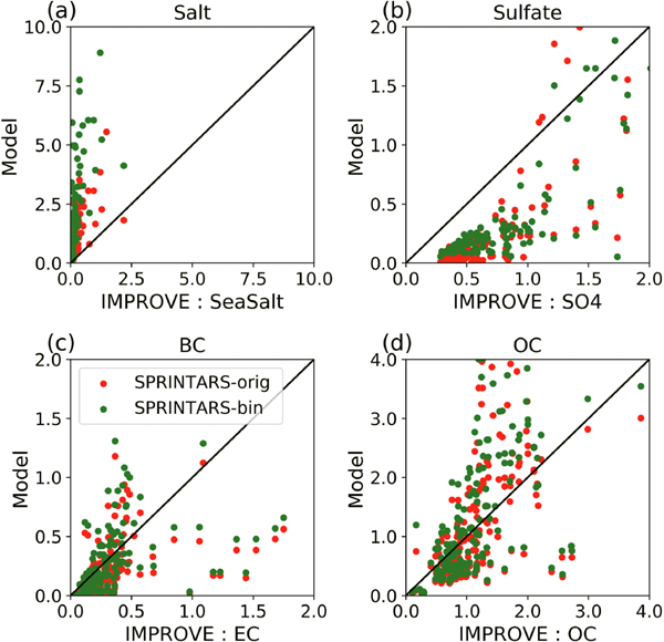
a. Comparisons of surface mass concentrations with IMPROVE
We compared the annually-averaged surface mass concentrations (Fig. 3) with the year 2006 data from the IMPROVE program (United States Interagency Monitoring of Protected Visual Environment; http://vista.cira.colostate.edu/improve). All stations are located in North America, and only the masses of fine particles (diameter < 2.5 µm) are considered. Figure 8 shows the scatter plots of the model results against IMPROVE measurements for four aerosol types: sea salt, sulfate, BC, and OC. As listed in Table 2, the model-observation correlations for sea salt are 0.68 and 0.70 for NICAM-SPRINTARS-orig and NICAM-SPRINTARS-bin, respectively. At the same time, the scatter plot (Fig. 8a) suggests that the surface sea salt masses are overestimated at 165 (NICAM-SPRINTARS-orig) and 169 (NICAM-SPRINTARS-bin) of the 170 stations, and NICAM-SPRINTARS-bin generally predicts higher values. This may be attributed to the fact that the emission of sea salt is sensitive to the wind speed that is not well resolved in the low horizontal resolution used in this study. On the other hand, the surface sulfate mass concentrations at the stations exhibit reasonable correlation coefficients (0.73 and 0.65 for NICAM-SPRINTARS-orig and NICAM-SPRINTARS-bin) but tend to be underestimated in both models (Fig. 8b). The correlation coefficients for BC (0.45) and OC (0.53) are lower. Both models underestimate the surface masses, and NICAM-SPRINTARS-bin predicts a smaller bias than NICAM-SPRINTARS-orig. Overall, both models reproduce the variations in surface mass concentrations in North America fairly well.
Following the previous model evaluation for global aerosol microphysics models (Bergman et al. 2012; Mann et al. 2014), we compared the simulated surface number concentrations with observations at 12 stations of GAW (Global Atmosphere Watch; https://community.wmo.int/activity-areas/gaw) that have a long measurement time series from Condensation Nucleus Counter (CNC) deployed at the station (for at least 15 years). Figure 9 shows the annual averages of the models plotted against the annual mean of the multi-year measurements with error bars showing the interannual variability. The total number concentrations from the models are calculated as the total number of particles above the threshold diameter specified by the particular CNC used at each station. It should be noted that the logarithmic scale is used for plotting and computing the statistics as the particle concentrations vary across several orders of magnitude.

The results indicate that NICAM-SPRINTARS-orig underestimates the total number concentrations at most of the stations: the values are underestimated by more than one order of magnitude at half of the stations. This can be attributed to the limitations of NICAM-SPRINTARS-orig in predicting the number concentration of fine particles, which usually dominates the total number concentrations. On the other hand, NICAM-SPRINTARS-bin tends to predict higher number concentrations of fine particles relative to coarse particles (Fig. 5). The model can reproduce the observed values within one order of magnitude at 11 out of the 12 stations. Figure 10 compares the monthly averages of number concentrations observed at GAW stations and simulated by the models. It is evident that NICAM-SPRINTARS-bin predicts values closer to observations at most of the stations, with NICAM-SPRINTARS-orig underestimating the number concentrations by more than an order of magnitude at several stations (e.g., Barrow, South Pole). The seasonal variations are also fairly well captured by NICAM-SPRINTARS-bin at some of the stations (e.g., Pallas, Neumayer). The size-resolving capacity of NICAM-SPRINTARS-bin thus greatly improves over the strong underprediction of total number concentrations predicted by NICAM-SPRINTARS-orig.

The EUSAAR (European Supersites for Atmospheric Aerosol Research; http://www.eusaar.net/) project provides harmonized aerosol measurement data from European field monitoring stations (Philippin et al. 2009). Asmi et al. (2011) analyzed the measured size-resolved number concentrations during 2008–09 and provided a convenient dataset for comparisons with models. In this study, we compare the model results with the surface number concentrations (Fig. 11) in three size classes defined by the dry diameter: between 30 nm and 50 nm (N30–50), larger than 50 nm (N50), and larger than 100 nm (N100). For the finest particles (N30–50), NICAM-SPRINTARS-orig underestimates the annually-averaged number concentrations at all stations: the values of 23 out of the 24 stations are lower than 10−1 of the observed values. On the other hand, NICAM-SPRINTARS-bin produces values closer to those observed, with values at 22 out of 24 stations within one order of magnitude of the observations (Fig. 11a). For the coarser particles (N50 and N100), the number concentrations simulated by both models are closer to observations than N30–50. The number concentrations of N50 predicted by NICAM-SPRINTARS-orig and NICAM-SPRINTARS-bin are within one order of magnitude of the observed values at 9 and 19 stations, but most of the values are underestimated. For N100, both models underestimate the number concentrations at all stations. The underestimated number concentrations of coarse particles may imply fewer potential CCN predicted in both models given the relevance of coarse particles to CCN (Andreae and Rosenfeld 2008).

To investigate the column-integrated optical properties of aerosols, we compare the model-simulated AOD and AE with two observational datasets from remote-sensing measurements: AERONET and MODIS. AERONET (AErosol RObotic NETwork) routinely provides quality-assured retrievals of AOD and AE from ground-based sky radiance measurements (Holben et al. 1998) and is often used for validation or calibration of satellite-retrieved aerosol products. We use the Level 2 daily average product to calculate the annual averages for the 144 stations with more than 100 days of valid data in the year 2006. To evaluate the global distribution of aerosol properties, we also calculate the annual average at each grid point using the Collection 6.1 Level 3 monthly products of AOD and AE (Platnick et al. 2015) measured by MODIS (Moderate Resolution Imaging Spectroradiometer). Wei et al. (2019) evaluated the performance of MODIS/Terra and MODIS/Aqua Collection 6.1 monthly AOD and found that neither instrument consistently outperforms the other over land. To increase the reliability of the comparisons to the satellite aerosol measurements, we compared the model results to the mean of the aerosol optical depths values from the two instruments.
The AODs predicted by both models at the AERONET stations are similar at most of the stations (Fig. 12a). The AODs predicted by NICAM-SPRINTARS-bin at over 93 % of the stations are within 0.5 times to 2 times of the values predicted by NICAM-SPRINTARS-orig. This is consistent with the similar mass concentrations simulated in the models (Figs. 3, 4). The different AODs can also be attributed to differences in underlying size distributions and the ways to calculate extinction coefficients. The aerosol masses at most of the stations are dominated by soil dust. It is also treated with the sectional method in SPRINTARS-orig, which explains why the two models produce similar values of AOD. Both models give high correlations with the AERONET-observed values and small negative bias, with a higher correlation simulated by NICAM-SPRINTARS-orig (0.65 vs. 0.64) but smaller bias by NICAM-SPRINTARS-bin (−0.16 vs. −0.04).

On the other hand, the Angstrom Exponent (AE) simulated at the stations exhibit very different behaviors in the two models. NICAM-SPRINTARS-orig underestimates the AE at most of the stations, and the correlation coefficient is 0.29. The underestimation of AE by NICAM-SPRINTARS-orig is also reported in a previous study (Dai et al. 2014). This suggests that SPRINTARS-orig tends to overestimate the particle sizes, as the finest particles are removed at the same rate as the larger ones in the bulk scheme. The correlation coefficient increased to 0.45 by resolving the size and aerosol microphysics in NICAM-SPRINTARS-bin. The annual averages of AE still tend to be under-estimated but to a smaller extent. Overall, NICAM-SPRINTARS-bin gives better agreement for this size-relevant metric.
The annual means of AOD and AE observed by MODIS are shown in Figs. 7a and 7d. High AOD (∼ 0.6) are observed over North Africa, accompanied by low AE (< 0.6). This can be explained by the emission of coarse soil dust particles from the Sahara desert. Similar results in this region are also reproduced by both NICAM-SPRINTARS-orig and NICAM-SPRINTARS-bin. The soil dust is transported across the Atlantic Ocean, creating a low AE belt near the equator. Both models predict the westward transport of soil dust, but the belt is not apparent over the ocean. In MODIS, the high AOD region extends westward and reaches the Caribbean Sea, but those simulated by both models are shifted northward. Biomass burning in Central Africa explains the AOD peak (∼ 0.5) as well as the high AE (> 1.5) in the southern part of Africa, as observed by MODIS. The models also simulate the AOD peak in central Africa, but AE in the southern part of Africa is lower than the values observed by MODIS.
The high AOD values over China observed by MODIS are suggested to be contributed by both soil dust from deserts and anthropogenic emissions from industrial areas (Luo et al. 2014). The high AE (above 1.2) observed in this region suggests that it is dominated by fine particles, including sulfate and carbonaceous aerosols. Both models simulate the AOD peak in China, but the AE is underestimated, and the values are similar to those over the Sahara Desert. The model-predicted AOD peaks are dominated by the presence of soil dust, and the contributions of aerosols from anthropogenic emissions are not well captured by the models.
In general, both models predict lower AOD in the industrial regions. For example, AOD and AE peaks are observed over the Middle East, India, and near Brazil by MODIS, but the models tend to underestimate the peak values, with NICAM-SPRINTARS-bin predicting lower values. The AE is also underestimated, but NICAM-SPRINTARS-bin gives values that are closer to the observations. The model-observation discrepancy may be explained by the limitations of the coarse grid resolution in mapping the emission inventories. The underestimation may also be partly attributed to the missing contribution of nitrate-containing aerosols, as suggested in previous studies using the SPRINTARS model (Dai et al. 2018; Park et al. 2018). The aging of BC by the condensation and coagulation by non-BC species are not simulated in the model, which may also lead to underestimated AOD at regions away from the BC sources.
The MODIS analysis suggests that the AOD over most of the oceans is lower than 0.2, but peaks with values up to 0.4 are simulated by the models. This may indicate that the sea salt burden may be overestimated, as positive bias is found in the sea salt mass concentrations at the IMPROVE stations. Values higher than 0.4 are observed by MODIS over the East China Sea, Sea of Japan, and the Sea of Okhotsk. The models also reproduce this high AOD region and suggest that the major contribution is from soil dust transported from China. The observed AE is about 0.9–1.2 in these regions, and NICAM-SPRINTARS-bin simulates closer values to observations compared to NICAM-SPRINTARS-orig. At high-latitude regions, including Russia and Canada, NICAM-SPRINTARS-bin predicts very high values of AE (> 1.8) due to the long-range transport of fine particles, which is not observed by MODIS.
5. Discussions
In general, the results from NICAM-SPRINTARS-bin are in reasonable agreement with the benchmark in situ and remote sensing aerosol observations that have been used to evaluate global aerosol microphysics models (e.g., Mann et al. 2014). In particular, the comparisons show that NICAM-SPRINTARS-bin improves the prediction of quantities that are more relevant to aerosol sizes, including the number concentration and Angstrom Exponent. It implies that the underlying size distributions are better captured by NICAM-SPRINTARS-bin. The size information from the size-resolving models may also be useful for other physical processes, such as the total surface area for chemical reactions in the chemistry module, the size-dependent optical properties for the radiation scheme, and the number concentration of CCN for cloud microphysics.
We acknowledge that the use of a size-resolving aerosol model alone is not sufficient to produce size distributions as observed in the field. The introduction of a size-resolving scheme in this study should be viewed as a framework that enables the implementations and testing of different parameters of aerosol properties and microphysics schemes suggested from observations and experiments. Thus, it is important to discuss potential factors that may affect the predicted size distributions and thus should be considered in future studies.
5.1 Choices of model parameters and emission schemes
This study focuses on the sensitivity of SPRINTARS to the size representation scheme and the introduction of aerosol dynamical processes. For consistency between the two versions of the model, assumptions in SPRINTARS-orig are also made in SPRINTARS-bin when possible, but these assumptions may not be optimized to produce the most realistic aerosol size distributions. For example, the size ranges of dust and salt are set between 0.2 µm to 20 µm, implying that the finer particles are not captured, and the long-range transport of these aerosols may be underestimated. Also, we followed the same emission schemes for salt and dust as in SPRINTARS-orig, but there are many other schemes proposed. Grythe et al. (2014) evaluated 21 different salt source functions and found significant variabilities in sea salt burdens. They also suggested that the dependency on sea surface temperature should be considered, which may explain the unexpected peak of sea salt mass in the Arctic region simulated in both models. For soil dust, several source functions are also proposed based on measurements as well as experimental studies, and the sensitivities to the source functions should also be investigated.
5.2 Aerosol mixing state
In both SPRINTARS-orig and SPRINTARS-bin, the major aerosol types are represented as external mixtures, which involve simulating particles as consisting of one particular type of aerosol. In the ambient atmosphere, however, aerosols usually exist as internal mixtures of different chemical compositions, for example, from the condensation of sulfuric acid and organics. In order to focus on the effect of size representations, and for a fair comparison with the existing non-microphysical scheme, we did not introduce new internal mixture components to SPRINTARS-bin in this study. We note that the skill score compared to the observations is likely affected by the externally mixed simplification.
In particular, the simulated sulfate aerosol sizes may deviate from the observed size distributions due to the mixed-type coagulation and other growth processes that are not implemented in the model. Limited by the external mixture assumption, the coagulation between particles of different aerosol types is not considered. Scavenging by larger particles is an important sink of the finest sulfate particles, and the absence of this effect in these simulations affects the particle number concentrations predicted by NICAM-SPRINTARS-bin. Coagulation with larger sulfate particles is, however, resolved in the simulations here and found to contribute to more than 50 % of the total global sink of sulfate particles with diameters smaller than 10 nm, and more than 30 % for those with diameters between 10 nm and 30 nm. The coagulation of sulfate with other aerosol types would lead to faster removal of fine particles and the formation of larger particles of higher extinction efficiencies. Besides, the growth processes of sulfate involving other chemical components are not considered in the current model. For example, SOA may condense on the existing sulfate particles, forming larger particles. These missing processes may explain the relatively low AOD values found in industrial regions, where both sulfate and carbonaceous aerosols dominate. The simplified mixing state will likely have led to an overpredicted atmospheric lifetime of fine sulfate particles, resulting in a high number concentrations and Angstrom Exponent at locations distant from the sources. This may explain the overestimated total number concentrations predicted at certain GAW stations (e.g., Bondville and Pallas, Fig. 10), as well as the high Angstrom Exponent, predicted in the high-latitude region (Fig. 7).
Another potential source of error from the externally mixed approach is in the BC mixing state, which is always 100 % black carbon (pure soot) in the current model. Freshly emitted BC particles mostly contain elemental carbon, so they are hydrophobic. In reality, emitted BC particles are gradually coated with other non-BC species, including sulfate and SOA, through coagulation and condensation, as well as photochemical oxidation processes. The internal mixing with non-BC material increases the absorption efficiencies (lensing effect) as well as the hygroscopicities. Bond et al. (2006) suggested that the absorption of aged aerosols is 50 % higher than fresh aerosols, although their results also suggested that the estimate of absorption enhancement also depends on the assumed mixing rules and geometries. Since the mixing of BC with sulfate and OC is not considered in the current model, the absorption enhancement due to BC aging is not captured, and the AOD contributed by BC is likely to be underestimated when the BC particles are far from the source regions. Thus, the BC mixing state should be considered a priority to include in the onward development of SPRINTARS-bin.
5.3 Model resolution
An advantage of the microphysical model being developed in NICAM-SPRINTARS, is that the model can be seamlessly run for a wide range of different grid resolutions. However, minimizing model-observation discrepancies is not the purpose of this study, so we used the relatively coarse grid resolution for climate simulations and have demonstrated that NICAM-SPRINTARS-bin can still produce reasonable results over the globe at this resolution. It is expected that the low resolution of the grid limits the accuracies in reproducing the observations because the meteorological fields only represent the mean state of regions of hundreds of square kilometers the local terrains are not well resolved. Consequently, the aerosol transport may not reflect the actual transport at measurement stations. In addition, errors are introduced when the emission inventories are mapped on a coarser grid, including the emission strengths and locations. These effects tend to dilute the chemistry and aerosol processes, affecting the spatial distributions of aerosols and also the size distributions of sulfate particles. For example, larger particles are likely to be produced under higher gaseous sulfate concentrations (due to stronger growth).
In the cloud-resolving experiments of NICAM-SPRINTARS, cloud processes can be explicitly simulated without the use of cumulus parameterizations. The more realistic simulation of cloud structure and precipitation without changing the source code makes NICAM-SPRINTARS suitable for the investigation of aerosol-cloud interactions over multiple scales. The influence of aerosol concentrations and size distributions on cloud systems has been recognized (e.g., Tao et al. 2007; Ekman et al. 2011). It is also suggested that the size representations affect the accuracy in modeling aerosol-cloud interactions (Zhang et al. 2002). However, size-resolving aerosol schemes have been rarely used in cloud-resolving simulations (e.g., Ekman et al. 2006). It is expected that high-resolution experiments using NICAM-SPRINTARS-bin introduced here provide new opportunities to understand aerosol-cloud interactions from a global perspective.
5.4 Aerosol-cloud interactions
To investigate the potential impact on aerosol-cloud interactions by the size-resolving model, we calculate the activation diameters (minimum diameter of aerosols to be activated) of different aerosol types using the schemes proposed in Abdul-Razzak and Ghan (2000, 2002). The scheme has been proposed for the use of multiple aerosol populations represented by size bins and considers the supersaturation, updraft velocities, aerosol hygroscopicity as well as the size distributions of all aerosols simulated in the model. These online-calculated activation diameters are not used in calculating in-cloud scavenging and cloud activation processes (Section 3.5a), and thus should be regarded as an initial investigation of size dependencies and variabilities of the CCN properties in global model simulations.
As shown in Fig. 13, the activation diameters are highly variable, which is not likely to be captured by SPRINTARS-orig. At low altitudes, the activation diameters are mainly within the smallest size bins, and the whole aerosol populations are likely to be activated. The activation diameters tend to increase with increasing altitude for the activation diameters of sulfate and OC, for instance, mostly above 200 nm at 7 km (Figs. 13c, d). Thus, it is expected that SPRINTARS-bin can better capture the effect of aerosols on cloud microphysics when used in high-resolution simulations. It should be noted that the activation diameters calculated here are only an estimation because the updraft velocities are not well resolved in this low-resolution experiment. By combining the size distributions and the resolved updraft velocities provided by the cloud-resolving NICAM model, the number concentrations of CCN being activated can be better estimated. The more accurate calculation of CCN activation also affects the size distributions of aerosols due to in-cloud scavenging and recycling processes (Ekman et al. 2011). Such consideration of recycling of aerosols from cloud evaporation is possible only when a detailed cloud microphysics scheme is used.

6. Summary
We implemented a full sectional microphysics scheme (SPRINTARS-bin) into the aerosol model SPRINTARS and evaluated its predictions within climate-resolution simulations in the global model NICAM. To investigate the fundamental differences in the model behaviors, assumptions in the original SPRINTARS model (SPRINTARS-orig) are followed when possible. As the same emission inventories or emission schemes are used, and the wind fields are nudged to a meteorological re-analysis, the overall aerosol burden does not differ substantially between the two models, resulting in similar distributions of surface mass concentrations and aerosol optical depth.
In SPRINTARS-orig, size distributions of soil dust and sea salt are represented by 10 and 4 size bins, respectively, whereas 20 bins are used to resolve the size distribution of each aerosol component in SPRINTARS-bin. Therefore, different behaviors between the two models are principally attributed to the size distribution resolution of these two types of coarse particles. For carbonaceous aerosols, the initial size distribution in SPRINTARS-bin is assumed to be the same as the prescribed log-normal distribution in SPRINTARS-orig, so that the differences are mostly due to size-dependencies of the deposition processes. The overall picture for these three aerosol types is not greatly changed, although NICAM-SPRINTARS-bin predicts vertical transport to slightly higher levels. In the microphysical approach of SPRINTARS-bin, the size distribution of sulfate is entirely determined from aerosol microphysical processes (e.g., nucleation, coagulation, and condensation). As a result, the two models demonstrate different sulfate transport within NICAM due to the different size representations of sulfate particles. Particularly, NICAM-SPRINTARS-bin simulated a stronger transport of finest particles to regions remote from sources of pollution.
The largest differences between the two models are seen in the more size-relevant quantities: number concentrations and Angstrom Exponent (AE). The number concentrations are highly sensitive to the presence of ultra-fine aerosol particles. As NICAM-SPRINTARS-orig does not resolve the size distributions of sulfate and carbonaceous aerosols, the number concentrations at GAW and EUSAAR stations are strongly underestimated. By contrast, NICAM-SPRINTARS-bin resolves new particle formation and coagulation and predicts much higher number concentrations as the finest particles are resolved. These fine particles are transported to the Arctic and Antarctica. Comparison with observations demonstrates that NICAM-SPRINTARS-bin improves the estimation of total number concentrations at GAW stations, number concentrations of fine particles at EUSAAR stations, as well as the AE values closer to the observations in AERONET. However, the performance in predicting the number concentrations of coarse particles, which have a higher potential to act as CCN in warm clouds, is not greatly improved.
Although the simulations are run at a climate-scale resolution and with model parameters that have not yet been optimized, the results are generally in good agreement with different observations. The model-observation differences highlight the need for sensitivity experiments to test different schemes and parameter settings within uncertainties to seek more realistic simulations of aerosol size distributions. The evaluation suggests that internally-mixed aerosol components and BC aging should also be included. SPRINTARS-bin provides a framework to incorporate improved size-dependent representations of aerosol processes, including more sophisticated emission mechanisms and source functions, cloud activation schemes, and aerosol nucleation schemes. The size information is also expected to improve our knowledge in understanding and quantifying the interactions of aerosols with radiation and clouds.
Supplements
Supplementary Table S1 shows the computation time ratios and total AOD root-mean-square deviation for a set of 1-week long simulations using NICAM-SPRINTARS-orig and NICAM-SPRINTARS-bin with different numbers of bins. Supplementary Tables S2 and S3 show the growth factor parameters and refractive indices used in the simulations, respectively.
Acknowledgments
We are thankful to Dr. D. Goto of NIES, Japan, for providing us with the emission datasets and share his insights. We would also like to thank Dr. T. Dai of the Chinese Academy of Sciences and Dr. T. Takemura of Kyushu University, Japan, for their assistance during this research. We are also grateful to two anonymous reviewers for their valuable comments that greatly helped improve the manuscript. We are immensely grateful to the researchers who provided the observation datasets: AERONET (https://aeronet.gsfc.nasa.gov/), MODIS Aerosol Product (https://modis.gsfc.nasa.gov/data/dataprod/mod08.php), GAW (https://www.gaw-wdca.org/), EUSAAR (http://www.eusaar.net) and NCEP FNL reanalysis data. We thank A. Asmi for permission to use their 2-year harmonized dataset of EUSAAR measurements (https://doi.pangaea.de/10.1594/PANGAEA.861856). This study was supported by JSPS KAKENHI Grant Number (19H05669, 19H05699), Program for Promoting Researches on the Supercomputer Fugaku (Large Ensemble Atmospheric and Environmental Prediction for Disaster Prevention and Mitigation) of MEXT (JPMXP1020351142), and JAXA/GCOM-C. Model simulations are performed using supercomputer resources Oakforest-PACS (The University of Tokyo, Japan).
Data Availability Statement
The data analysis files are available in J-STAGE Data. https://doi.org/10.34474/data.jmsj.14479557
References
- Abdul-Razzak, H., and S. J. Ghan, 2000: A parameterization of aerosol activation. 2. Multiple aerosol types. J. Geophys. Res., 105, 6837-6844.
- Abdul-Razzak, H., and S. J. Ghan, 2002: A parameterization of aerosol activation. 3. Sectional representation. J. Geophys. Res., 107, 4026, doi:10.1029/2001JD000483.
- Abdul-Razzak, H., S. J. Ghan, and C. Rivera-Carpio, 1998: A parameterization of aerosol activation. 1. Single aerosol type. J. Geophys. Res., 103, 6123-6131.
- Adams, P. J., and J. H. Seinfeld, 2002: Predicting global aerosol size distributions in general circulation models. J. Geophys. Res., 107, 4370, doi:10.1029/2001JD001010.
- Alfaro, S. C., and L. Gomes, 2001: Modeling mineral aerosol production by wind erosion: Emission intensities and aerosol size distributions in source areas. J. Geophys. Res., 106, 18075-18084.
- Andreae, M. O., and D. Rosenfeld, 2008: Aerosol–cloud–precipitation interactions. Part 1. The nature and sources of cloud-active aerosols. Earth-Sci. Rev., 89, 13-41.
- Anttila, T., V.-M. Kerminen, and K. E. J. Lehtinen, 2010: Parameterizing the formation rate of new particles: The effect of nuclei self-coagulation. J. Aerosol Sci., 41, 621-636.
- Asmi, A., A. Wiedensohler, P. Laj, A.-M. Fjaeraa, K. Sellegri, W. Birmili, E. Weingartner, U. Baltensperger, V. Zdimal, N. Zikova, J.-P. Putaud, A. Marinoni, P. Tunved, H.-C. Hansson, M. Fiebig, N. Kivekäs, H. Lihavainen, E. Asmi, V. Ulevicius, P. P. Aalto, E. Swietlicki, A. Kristensson, N. Mihalopoulos, N. Kalivitis, I. Kalapov, G. Kiss, G. de Leeuw, B. Henzing, R. M. Harrison, D. Beddows, C. O'Dowd, S. G. Jennings, H. Flentje, K. Weinhold, F. Meinhardt, L. Ries, and M. Kulmala, 2011: Number size distributions and seasonality of submicron particles in Europe 2008–2009. Atmos. Chem. Phys., 11, 5505-5538.
- Bates, T. S., R. J. Charlson, and R. H. Gammon, 1987: Evidence for the climatic role of marine biogenic sulphur. Nature, 329, 319-321.
- Bergman, T., V.-M. Kerminen, H. Korhonen, K. J. Lehtinen, R. Makkonen, A. Arola, T. Mielonen, S. Romakkaniemi, M. Kulmala, and H. Kokkola, 2012: Evaluation of the sectional aerosol microphysics module SALSA implementation in ECHAM5-HAM aerosol-climate model. Geosci. Model Dev., 5, 845-868.
- Bond, T. C., G. Habib, and R. W. Bergstrom, 2006: Limitations in the enhancement of visible light absorption due to mixing state. J. Geophys. Res., 111, D20211, doi:10.1029/2006JD007315.
- Boucher, O., D. Randall, P. Artaxo, C. S. Bretherton, G. Feingold, P. Forster, V.-M. Kerminen, Y. Kondo, H. Liao, U. Lohmann, P. Rasch, S. K. Satheesh, S. Sherwood, B. Stevens, X.-Y. Zhang, 2013: Clouds and aerosols. Climate Change 2013: The Physical Science Basis. Contribution of Working Group I to the Fifth Assessment Report of the Intergovernmental Panel on Climate Change. Stocker, T. F., D. Qin, G.-K. Plattner, M. Tignor, S. K. Allen, J. Boschung, A. Nauels, Y. Xia, V. Bex, and P.M. Midgley (eds.). Cambridge University Press, Cambridge, UK and New York, USA, 571-658.
- Ching, J., R. A. Zaveri, R. C. Easter, N. Riemer, and J. D. Fast, 2016: A three-dimensional sectional representation of aerosol mixing state for simulating optical properties and cloud condensation nuclei. J. Geophys. Res.: Atmos., 121, 5912-5929.
- d'Almeida, G. A., and L. Schütz, 1983: Number, mass and volume distributions of mineral aerosol and soils of the Sahara. J. Appl. Meteor. Climatol., 22, 233-243.
- d'Almeida, G. A., P. Koepke, and E. P. Shettle, 1991: Atmospheric Aerosols: Global Climatology and Radiative Characteristics. A Deepak Pub., 561 pp.
- Dai, T., D. Goto, N. A. J. Schutgens, X. Dong, G. Shi, and T. Nakajima, 2014: Simulated aerosol key optical properties over global scale using an aerosol transport model coupled with a new type of dynamic core. Atmos. Environ., 82, 71-82.
- Dai, T., Y. Cheng, P. Zhang, G. Shi, M. Sekiguchi, K. Suzuki, D. Goto, and T. Nakajima, 2018: Impacts of meteorological nudging on the global dust cycle simulated by NICAM coupled with an aerosol model. Atmos. Environ., 190, 99-115.
- Diehl, T., A. Heil, M. Chin, X. Pan, D. Streets, M. Schultz, and S. Kinne, 2012: Anthropogenic, biomass burning, and volcanic emissions of black carbon, organic carbon, and SO2 from 1980 to 2010 for hindcast model experiments. Atmos. Chem. Phys. Discuss., 12, 24895-24954.
- Ekman, A. M. L., C. Wang, J. Ström, and R. Krejci, 2006: Explicit simulation of aerosol physics in a cloud-resolving model: Aerosol transport and processing in the free troposphere. J. Atmos. Sci., 63, 682-696.
- Ekman, A. M. L., A. Engström, and A. Söderberg, 2011: Impact of two-way aerosol-cloud interaction and changes in aerosol size distribution on simulated aerosol-induced deep convective cloud sensitivity. J. Atmos. Sci., 68, 685-698.
- Fan, J., Y. Wang, D. Rosenfeld, and X. Liu, 2016: Review of aerosol-cloud interactions: Mechanisms, significance, and challenges. J. Atmos. Sci., 73, 4221-4252.
- Foret, G., G. Bergametti, F. Dulac, and L. Menut, 2006: An optimized particle size bin scheme for modeling mineral dust aerosol. J. Geophys. Res., 111, D17310, doi:10.1029/2005JD006797.
- Gong, S. L., 2003: A parameterization of sea-salt aerosol source function for sub-and super-micron particles. Global Biogeochem. Cycles, 17, 1097, doi:10.1029/2003GB002079.
- Gong, S. L., and L. A. Barrie, 2003: Simulating the impact of sea salt on global nss sulphate aerosols. J. Geophys. Res., 108, 4516, doi:10.1029/2002JD003181.
- Gong, S. L., L. A. Barrie, J.-P. Blanchet, K. von Salzen, U. Lohmann, G. Lesins, L. Spacek, L. M. Zhang, E. Girard, H. Lin, R. Leaitch, H. Leighton, P. Chylek, and P. Huang, 2003: Canadian Aerosol Module: A size-segregated simulation of atmospheric aerosol processes for climate and air quality models. 1. Module development. J. Geophys. Res., 108, 4007, doi:10.1029/2001JD002002.
- Goto, D., T. Nakajima, T. Takemura, and K. Sudo, 2011: A study of uncertainties in the sulfate distribution and its radiative forcing associated with sulfur chemistry in a global aerosol model. Atmos. Chem. Phys., 11, 10889-10910.
- Goto, D., T. Dai, M. Satoh, H. Tomita, J. Uchida, S. Misawa, T. Inoue, H. Tsuruta, K. Ueda, C. F. S. Ng, A. Takami, N. Sugimoto, A. Shimizu, T. Ohara, and T. Nakajima, 2015: Application of a global nonhydrostatic model with a stretched-grid system to regional aerosol simulations around Japan. Geosci. Model Dev., 8, 235-259.
- Goto, D., T. Nakajima, D. Tie, H. Yashiro, Y. Sato, K. Suzuki, J. Uchida, S. Misawa, R. Yonemoto, T. T. N. Trieu, H. Tomita, and M. Satoh, 2018: Multi-scale simulations of atmospheric pollutants using a nonhydrostatic icosahedral atmospheric model. Land-Atmospheric Research Applications in South and Southeast Asia. Vadrevu, K., T. Ohara, and C. Justice (eds.), Springer, Cham, 277-302.
- Goto, D., M. Kikuchi, K. Suzuki, M. Hayasaki, M. Yoshida, T. M. Nagao, M. Choi, J. Kim, N. Sugimoto, A. Shimizu, E. Oikawa, and T. Nakajima, 2019: Aerosol model evaluation using two geostationary satellites over East Asia in May 2016. Atmos. Res., 217, 93-113.
- Goto, D., Y. Sato, H. Yashiro, K. Suzuki, E. Oikawa, R. Kudo, T. M. Nagao, and T. Nakajima, 2020: Global aerosol simulations using NICAM.16 on a 14 km grid spacing for a climate study: Improved and remaining issues relative to a lower-resolution model. Geosci. Model Dev., 13, 3731-3768.
- Grythe, H., J. Ström, R. Krejci, P. Quinn, and A. Stohl, 2014: A review of sea-spray aerosol source functions using a large global set of sea salt aerosol concentration measurements. Atmos. Chem. Phys., 14, 1277-1297.
- Haywood, J., and O. Boucher, 2000: Estimates of the direct and indirect radiative forcing due to tropospheric aerosols: A review. Rev. Geophys., 38, 513-543.
- Holben, B. N., T. F. Eck, I. Slutsker, D. Tanré, J. P. Buis, A. Setzer, E. Vermote, J. A. Reagan, Y. J. Kaufman, T. Nakajima, F. Lavenu, I. Jankowiak, and A. Smirnov, 1998: AERONET —A federated instrument network and data archive for aerosol characterization. Remote Sens. Environ., 66, 1-16.
- Jacobson, M. Z., 1997a: Development and application of a new air pollution modeling system—II. Aerosol module structure and design. Atmos. Environ., 31, 131-144.
- Jacobson, M. Z., 1997b: Numerical techniques to solve condensational and dissolutional growth equations when growth is coupled to reversible reactions. Aerosol Sci. Technol., 27, 491-498.
- Jacobson, M. Z., 2005: Coagulation. Fundamentals of Atmospheric Modeling. 2nd Edition. Cambridge University Press, 494-524.
- Jacobson, M. Z., R. P. Turco, E. J. Jensen, and O. B. Toon, 1994: Modeling coagulation among particles of different composition and size. Atmos. Environ., 28, 1327-1338.
- Janssens-Maenhout, G., M. Crippa, D. Guizzardi, F. Dentener, M. Muntean, G. Pouliot, T. Keating, Q. Zhang, J. Kurokawa, R. Wankmüller, H. Denier van der Gon, J. J. P. Kuenen, Z. Klimont, G. Frost, S. Darras, B. Koffi, and M. Li, 2015: HTAP_v2.2: A mosaic of regional and global emission grid maps for 2008 and 2010 to study hemispheric transport of air pollution. Atmos. Chem. Phys., 15, 11411-11432.
- Kerminen, V.-M., and M. kulmala, 2002: Analytical formulae connecting the “real” and the “apparent” nucleation rate and the nuclei number concentration for atmospheric nucleation events. J. Aerosol Sci., 33, 609-622.
- Kodama, C., Y. Yamada, A. T. Noda, K. Kikuchi, Y. Kajikawa, T. Nasuno, T. Tomita, T. Yamaura, H. G. Takahashi, M. Hara, Y. Kawatani, M. Satoh, and M. Sugi, 2015: A 20-year climatology of a NICAM AMIP-type simulation. J. Meteor. Soc. Japan, 93, 393-424.
- Kok, J. F., 2011a: A scaling theory for the size distribution of emitted dust aerosols suggests climate models underestimate the size of the global dust cycle. Proc. Natl. Acad. Sci. U. S. A., 108, 1016-1021.
- Kok, J. F., 2011b: Does the size distribution of mineral dust aerosols depend on the wind speed at emission?
Atmos. Chem. Phys., 11, 10149-10156.
- Kokkola, H., H. Korhonen, K. E. J. Lehtinen, R. Makkonen, A. Asmi, S. Järvenoja, T. Anttila, A.-I. Partanen, M. Kulmala, H. Järvinen, A. Laaksonen, and V.-M. Kerminen, 2008: SALSA — A sectional aerosol module for large scale applications. Atmos. Chem. Phys., 8, 2469-2483.
- Kokkola, H., T. Kühn, A. Laakso, T. Bergman, K. E. J. Lehtinen, T. Mielonen, A. Arola, S. Stadtler, H. Korhonen, S. Ferrachat, U. Lohmann, D. Neubauer, I. Tegen, C. S.-L. Drian, M. G. Schultz, I. Bey, P. Stier, N. Daskalakis, C. L. Heald, and S. Romakkaniemi, 2018: SALSA2.0: The sectional aerosol module of the aerosol-chemistry-climate model ECHAM6.3.0-HAM2.3-MOZ1.0. Geosci. Model Dev., 11, 3833-3863.
- Kulmala, M., A. Laaksonen, and L. Pirjola, 1998: Parameterizations for sulfuric acid/water nucleation rates. J. Geophys. Res., 103, 8301-8307.
- Kulmala, M., K. E. J. Lehtinen, and A. Laaksonen, 2006: Cluster activation theory as an explanation of the linear dependence between formation rate of 3 nm particles and sulphuric acid concentration. Atmos. Chem. Phys., 6, 787-793.
- Lee, Y. H., and P. J. Adams, 2012: A fast and efficient version of the TwO-Moment Aerosol Sectional (TOMAS) global aerosol microphysics model. Aerosol Sci. Technol., 46, 678-689.
- Lehtinen, K. E. J., M. Dal Maso, M. Kulmala, and V.-M. Kerminen, 2007: Estimating nucleation rates from apparent particle formation rates and vice versa: Revised formulation of the Kerminen-Kulmala equation. J. Aerosol Sci., 38, 988-994.
- Lohmann, U., and J. Feichter, 2005: Global indirect aerosol effects: A review. Atmos. Chem. Phys., 5, 715-737.
- Luo, Y., X. Zheng, T. Zhao, and J. Chen, 2014: A climatology of aerosol optical depth over China from recent 10 years of MODIS remote sensing data. Int. J. Climatol., 34, 863-870.
- Määttänen, A., J. Merikanto, H. Henschel, J. Duplissy, R. Makkonen, I. K. Ortega, and H. Vehkamäki, 2018: New parameterizations for neutral and ion-induced sulfuric acid-water particle formation in nucleation and kinetic regimes. J. Geophys. Res.: Atmos., 123, 1269-1296.
- Mann, G. W., K. S. Carslaw, D. V. Spracklen, D. A. Ridley, P. T. Manktelow, M. P. Chipperfield, S. J. Pickering, and C. E. Johnson, 2010: Description and evaluation of GLOMAP-mode: A modal global aerosol microphysics model for the UKCA composition-climate model. Geosci. Model Dev., 3, 519-551.
- Mann, G. W., K. S. Carslaw, D. A. Ridley, D. V. Spracklen, K. J. Pringle, J. Merikanto, H. Korhonen, J. P. Schwarz, L. A. Lee, P. T. Manktelow, M. T. Woodhouse, A. Schmidt, T. J. Breider, K. M. Emmerson, C. L. Reddington, M. P. Chipperfield, and S. J. Pickering, 2012: Intercomparison of modal and sectional aerosol microphysics representations within the same 3-D global chemical transport model. Atmos. Chem. Phys., 12, 4449-4476.
- Mann, G. W., K. S. Carslaw, C. L. Reddington, K. J. Pringle, M. Schulz, A. Asmi, D. V. Spracklen, D. A. Ridley, M. T. Woodhouse, L. A. Lee, K. Zhang, S. J. Ghan, R. C. Easter, X. Liu, P. Stier, Y. H. Lee, P. J. Adams, H. Tost, J. Lelieveld, S. E. Bauer, K. Tsigaridis, T. P. C. van Noije, A. Strunk, E. Vignati, N. Bellouin, M. Dalvi, C. E. Johnson, T. Bergman, H. Kokkola, K. von Salzen, F. Yu, G. Luo, A. Petzold, J. Heintzenberg, A. Clarke, J. A. Ogren, J. Gras, U. Baltensperger, U. Kaminski, S. G. Jennings, C. D. O'Dowd, R. M. Harrison, D. C. S. Beddows, M. Kulmala, Y. Viisanen, V. Ulevicius, N. Mihalopoulos, V. Zdimal, M. Fiebig, H.-C. Hansson, E. Swietlicki, and J. S. Henzing, 2014: Intercomparison and evaluation of global aerosol microphysical properties among AeroCom models of a range of complexity. Atmos. Chem. Phys., 14, 4679-4713.
- Maring, H., D. L. Savoie, M. A. Izaguirre, L. Custals, and J. S. Reid, 2003: Mineral dust aerosol size distribution change during atmospheric transport. J. Geophys. Res., 108, 8592, doi:10.1029/2002JD002536.
- Marti, J. J., A. Jefferson, X. P. Cai, C. Richert, P. H. Mc-Murry, and F. Eisele, 1997: H2SO4 vapor pressure of sulfuric acid and ammonium sulfate solutions. J. Geophys. Res., 102, 3725-3735.
- Matsui, H., 2017: Development of a global aerosol model using a two-dimensional sectional method: 1. Model design. J. Adv. Model. Earth Syst., 9, 1921-1947.
- Matsui, H., and N. Mahowald, 2017: Development of a global aerosol model using a two-dimensional sectional method: 2. Evaluation and sensitivity simulations. J. Adv. Model. Earth Syst., 9, 1887-1920.
- Matsui, H., M. Koike, Y. Kondo, J. D. Fast, and M. Takigawa, 2014: Development of an aerosol microphysical module: Aerosol Two-dimensional bin module for foRmation and Aging Simulation (ATRAS). Atmos. Chem. Phys., 14, 10315-10331.
- Miura, H., M. Satoh, T. Nasuno, A. T. Noda, and K. Oouchi, 2007: A Madden-Julian Oscillation event realistically simulated by a global cloud-resolving model. Science, 318, 1763-1765.
- Miyamoto, Y., Y. Kajikawa, R. Yoshida, T. Yamaura, H. Yashiro, and H. Tomita, 2013: Deep moist atmospheric convection in a subkilometer global simulation. Geophys. Res. Lett., 40, 4922-4926.
- Monahan, E. C., D. E. Spiel, and K. L. Davidson, 1986: A model of marine aerosol generation via whitecaps and wave disruption. Oceanic Whitecaps: And Their Role in Air-Sea Exchange Processes. Monahan, E. C., and G. M. Niocaill (eds.), Springer, Dordrecht, 167-174.
- NOAA/NCEP, 2000: NCEP FNL Operational Model Global Tropospheric Analyses, continuing from July 1999. Res. Data Arch. Natl. Cent. Atmos. Res. Comput. Inf. Syst. Lab., ds083.2, doi:10.5065/D6M043C6.
- Park, S. S., T. Takemura, and S.-W. Kim, 2018: Comparison of aerosol optical depth between observation and simulation from MIROC-SPRINTARS: Effects of temporal inhomogeneous sampling. Atmos. Environ., 186, 56-73.
- Philippin, S., P. Laj, J.-P. Putaud, A. Wiedensohler, G. De Leeuw, A. M. Fjaeraa, U. Platt, U. Baltensperger, and M. Fiebig, 2009: EUSAAR—An unprecedented network of aerosol observation in Europe. Earozoru Kenkyu, 24, 78-83.
- Platnick, S., M. D. King, K. G. Meyer, G. Wind, N. Amarasinghe, B. Marchant, G. T. Arnold, Z. Zhang, P. A. Hubanks, B. Ridgway, and J. Riedi, 2015: MODIS atmosphere L3 monthly product. The Level-3 MODIS Atmosphere Daily Global Product, NASA MODIS Adaptive Processing System, Goddard Space Flight Center, USA, doi:10.5067/MODIS/MOD08_M3.006.
- Sato, Y., D. Goto, T. Michibata, K. Suzuki, T. Takemura, H. Tomita, and T. Nakajima, 2018: Aerosol effects on cloud water amounts were successfully simulated by a global cloud-system resolving model. Nat. Commun., 9, 985, doi:10.1038/s41467-018-03379-6.
- Satoh, M., T. Matsuno, H. Tomita, H. Miura, T. Nasuno, and S. Iga, 2008: Nonhydrostatic icosahedral atmospheric model (NICAM) for global cloud resolving simulations. J. Comput. Phys., 227, 3486-3514.
- Satoh, M., H. Tomita, H. Yashiro, H. Miura, C. Kodama, T. Seiki, A. T. Noda, Y. Yamada, D. Goto, M. Sawada, T. Miyoshi, Y. Niwa, M. Hara, T. Ohno, S. Iga, T. Arakawa, T. Inoue, and H. Kubokawa, 2014: The nonhydrostatic icosahedral atmospheric model: Description and development. Prog. Earth Planet. Sci., 1, 18, doi:10.1186/s40645-014-0018-1.
- Satoh, M., B. Stevens, F. Judt, M. Khairoutdinov, S.-J. Lin, W. M. Putman, and P. Düben, 2019: Global cloud-resolving models. Curr. Climate Change Rep., 5, 172-184.
- Schulz, M., Y. J. Balkanski, W. Guelle, and F. Dulac, 1998: Role of aerosol size distribution and source location in a three-dimensional simulation of a Saharan dust episode tested against satellite-derived optical thickness. J. Geophys. Res., 103, 10579-10592.
- Spracklen, D. V., K. J. Pringle, K. S. Carslaw, M. P. Chipperfield, and G. W. Mann, 2005: A global off-line model of size-resolved aerosol microphysics: I. Model development and prediction of aerosol properties. Atmos. Chem. Phys., 5, 2227-2252.
- Stevens, B., and S. Bony, 2013: What are climate models missing? Science, 340, 1053-1054.
- Sudo, K., M. Takahashi, J. Kurokawa, and H. Akimoto, 2002: CHASER: A global chemical model of the troposphere. 1. Model description. J. Geophys. Res., 107, 4339, doi:10.1029/2001JD001113.
- Suzuki, K., T. Nakajima, M. Satoh, H. Tomita, T. Takemura, T. Y. Nakajima, and G. L. Stephens, 2008: Global cloud-system-resolving simulation of aerosol effect on warm clouds. Geophys. Res. Lett., 35, L19817, doi:10.1029/2008GL035449.
- Takemura, T., H. Okamoto, Y. Maruyama, A. Numaguti, A. Higurashi, and T. Nakajima, 2000: Global three-dimensional simulation of aerosol optical thickness distribution of various origins. J. Geophys. Res., 105, 17853-17873.
- Takemura, T., T. Nakajima, A. Higurashi, S. Ohta, and N. Sugimoto, 2003: Aerosol distributions and radiative forcing over the Asian Pacific region simulated by Spectral Radiation-Transport Model for Aerosol Species (SPRINTARS). J. Geophys. Res., 108, 8659, doi: 10.1029/2002JD003210.
- Takemura, T., T. Nozawa, S. Emori, T. Y. Nakajima, and T. Nakajima, 2005: Simulation of climate response to aerosol direct and indirect effects with aerosol transport-radiation model. J. Geophys. Res., 110, D02202, doi:10.1029/2004JD005029.
- Tao, W.-K., X. Li, A. Khain, T. Matsui, S. Lang, and J. Simpson, 2007: Role of atmospheric aerosol concentration on deep convective precipitation: Cloudresolving model simulations. J. Geophys. Res., 112, D24S18, doi:10.1029/2007JD008728.
- Textor, C., M. Schulz, S. Guibert, S. Kinne, Y. Balkanski, S. Bauer, T. Berntsen, T. Berglen, O. Boucher, M. Chin, F. Dentener, T. Diehl, R. Easter, H. Feichter, D. Fillmore, S. Ghan, P. Ginoux, S. Gong, A. Grini, J. Hendricks, L. Horowitz, P. Huang, I. Isaksen, I. Iversen, S. Kloster, D. Koch, A. Kirkevåg, J. E. Kristjansson, M. Krol, A. Lauer, J. F. Lamarque, X. Liu, V. Montanaro, G. Myhre, J. Penner, G. Pitari, S. Reddy, Ø. Seland, P. Stier, T. Takemura, and X. Tie, 2006: Analysis and quantification of the diversities of aerosol life cycles within AeroCom. Atmos. Chem. Phys., 6, 1777-1813.
- Tomita, H., and M. Satoh, 2004: A new dynamical framework of nonhydrostatic global model using the icosahedral grid. Fluid Dyn. Res., 34, 357-400.
- Tomita, H., H. Miura, S. Iga, T. Nasuno, and M. Satoh, 2005: A global cloud-resolving simulation: Preliminary results from an aqua planet experiment. Geophys. Res. Lett., 32, L08805, doi:10.1029/2005GL022459.
- Uchida, J., M. Mori, H. Nakamura, M. Satoh, K. Suzuki, and T. Nakajima, 2016: Error and energy budget analysis of a nonhydrostatic stretched-grid global atmospheric model. Mon. Wea. Rev., 144, 1423-1447.
- Uchida, J., M. Mori, M. Hara, M. Satoh, D. Goto, T. Kataoka, K. Suzuki, and T. Nakajima, 2017: Impact of lateral boundary errors on the simulation of clouds with a nonhydrostatic regional climate model. Mon. Wea. Rev., 145, 5059-5082.
- van der Does, M., L. F. Korte, C. I. Munday, G.-J. A. Brummer, and J.-B. W. Stuut, 2016: Particle size traces modern Saharan dust transport and deposition across the equatorial North Atlantic. Atmos. Chem. Phys., 16, 13697-13710.
- Vehkamäki, H., M. Kulmala, I. Napari, K. E. J. Lehtinen, C. Timmreck, M. Noppel, and A. Laaksonen, 2002: An improved parameterization for sulfuric acid–water nucleation rates for tropospheric and stratospheric conditions. J. Geophys. Res., 107, 4622, doi:10.1029/2002JD002184.
- Wei, J., Y. Peng, J. Guo, and L. Sun, 2019: Performance of MODIS Collection 6.1 Level 3 aerosol products in spatial-temporal variations over land. Atmos. Environ., 206, 30-44.
- Weisenstein, D. K., J. E. Penner, M. Herzog, and X. Liu, 2007: Global 2-D intercomparison of sectional and modal aerosol modules. Atmos. Chem. Phys., 7, 2339-2355.
- Whitby, K. T., 1978: The physical characteristics of sulfur aerosols. Atmos. Environ., 12, 135-159.
- Yu, F., and G. Luo, 2009: Simulation of particle size distribution with a global aerosol model: Contribution of nucleation to aerosol and CCN number concentrations. Atmos. Chem. Phys., 9, 7691-7710.
- Zhang, Y., R. C. Easter, S. J. Ghan, and H. Abdul-Razzak, 2002: Impact of aerosol size representation on modeling aerosol-cloud interactions. J. Geophys. Res., 107, 4558, doi:10.1029/2001JD001549.


