Radiowave Scattering Characteristics of Melting Layer Measured by a Dual Ka-band Radar System

Abstract

Specific attenuation and equivalent radar reflectivity in a melting layer were measured using a dual Ka-band radar system. The system consists of two identically designed Ka-radars. When the two radars are arranged to face each other and a precipitation system comes between the two radars, they observe the system from opposite directions. The radar echoes suffer from rain attenuation, which appears symmetrically in both radar echo profiles. By differentiating measured radar reflectivity with range, the specific attenuation (k) can be estimated. After obtaining the specific attenuation, the equivalent radar reflectivity (Z_e) is estimated. Melting layer observations were conducted on a slope of Mt. Zao, Japan. In the melting layer, the specific attenuation and the equivalent radar reflectivity vary considerably along the radio path. The relationship between k and Z_e showed interesting characteristics that appear in a loop-shape on a k-Z_e diagram. A simple theoretical study using the Rayleigh and Mie scattering theories for melting snow spheres showed that the basic loop-shape is because of the change in permittivity of precipitation particles during melting. The loop-shape is greatly expanded by the change of the particle size. The Mie effect, which is significant for large precipitation particles, slightly modifies the loop-shape by reducing backscattering cross sections. The results also explain the shelf-like profile instead of the peak-like for Z_e.

1. Introduction

Global changes in the environment have attracted international attention, and changes in precipitation are being observed. For example, the number of severe storms has increased. Changes in precipitation impact ecosystems and human society. To predict the changes in precipitation in the future, a better understanding of global precipitation characteristics is essential. Thus, the Global Precipitation Measurement (GPM) project was designed and built (Hou et al. 2014; Nakamura 2021). The GPM is an international venture led by the U.S. National Aeronautics and Space Administration (NASA) and the Japan Aerospace Exploration Agency (JAXA). It is a multi-satellite system, and the core satellite of the GPM was launched from the Tanegashima Space Center, JAXA on 29 February 2014. The core satellite carries two instruments for precipitation measurements, the Dual-wavelength Precipitation Radar (DPR) and the GPM microwave radiometer (GMI). The DPR was developed by JAXA and the National Institute of Information and Communications Technology (NICT), Japan, and the GMI was developed by NASA. The DPR can directly observe three-dimensional precipitation systems, and can provide a reference data set to other instruments for precipitation measurements, such as microwave radiometers.

The coverage of the GPM system was extended from the TRMM coverage to high latitude regions, where it frequently snows. Snow rate or equivalent rain rate measurements by radars are more difficult compared with the liquid rain rate measurements because snow particles have more complicated radiowave scattering characteristics compared with rain drops. In very cold regions, snow is dry, whereas in warmer regions, it is often wet. For example, a large part of the snow in Japan is wet snow. Thus, wet snow observations are essential for measuring global precipitation. The wet snow, which contains partly melted snow particles, has much more complex radiowave scattering than dry snow.

When a radar operated in the S, C, or X-band observes stratiform precipitation systems, a strong echo layer, which is called a bright band, often appears. The lower frequency radar of the DPR is in the Ku-band and it also observes the bright band. The bright band corresponds to a melting layer containing wet snow. As precipitating particles change from solid to liquid while falling, the size, shape, and relative permittivity of the particles change, and the dropsize distribution also changes because the falling velocity changes due to the coalescence or breakup of the particles. Thus, complicated processes occur in the melting layer, and such processes have been the subject of many studies (e.g., Leary and Houze 1979; Fabry and Zawadzki 1995). The radio scattering characteristics were also widely studied (e.g., Kollias and Albrecht 2005; Li and Moisseev 2019; Johnson et al. 2016; Leinonen and von Leber 2018).

The DPR is a 13.6/35.5 GHz radar, whereas the 35 GHz (Ka-band) spaceborne precipitation radar is more advanced. The dual-wavelength rain retrievals are being developed even now (e.g., Seto et al. 2021; Kobayashi et al. 2021). For the full utilization of the 35 GHz radar, radiowave scattering characteristics of precipitation particles must be well understood. In the Ka-band, attenuation of the radiowaves is strong, and conventional Ka-band radars measure only combination of scattering and attenuation. It is important to separate the effects of scattering and attenuation for precise measurement using Ka-radars. To measure scattering and attenuation characteristics of precipitation particles, a dual Ka-band radar system (DKR) was developed by JAXA (Nakamura et al. 2011). This system consists of two identically designed Ka-band radars. When the two radars are arranged to face each other and a precipitation system comes between the two radars, the precipitation system is observed from opposite directions. From the two radar signatures, specific attenuation (k) and equivalent radar reflectivity (Z_e) can be estimated. This idea was applied to an observation with an airborne and ground-based 94 GHz cloud radars (Li et al. 2001). The DKR has also been used for snow observations and showed the scattering characteristics of snow particles (Nishikawa et al. 2015). As an extension of the snow observations, the DKR was used for melting layer observations.

Herein, some results of the melting layer observations are presented in terms of the k-Z_e relationship derived from the DKR. An interpretation of the scattering characteristics is included.

2. Observation

Melting layer observations with radars are usually performed in a vertically pointing or volume scanning mode. In the present cases, two radars observe a melting layer that comes between the radars as shown in Fig. 1. For this observation, mountain slopes were chosen as the observation sites.

Fig. 1.

Configuration of melting layer observations at Zao Mountain slope.

During the planning phase of the melting layer observation experiment, candidate locations in Japan were surveyed. There were several criteria for selection. The location must have: (1) sufficient height difference, (2) frequent snowfall, (3) sufficient separation of the radio path from the ground, (4) easy accessibility, (5) the electric power availability, (6) easy transportation, (7) legal acceptability, and (8) accommodations. A total of 76 candidate sites were surveyed from Kyushu Island to Hokkaido Island in Japan. The numbers of days of melting layer appearances in a year were estimated using the temperature data from ground stations of the Japan Meteorological Agency near the candidate locations. A slope of the Zao Mountain (approximately 38.1°N, 140.4°E) in Yamagata Prefecture, Japan, where a ski resort is located, was selected as the most suitable location. The location was ranked 9th for topography and 13th for days of melting layer appearances. Melting layers appeared 42 days a year, that is, 2, 10, 8, 3, 3, 8, 8 days from October to April, respectively. The days in January and February are short because the temperature is too low for the melting layer to appear between the two radars.

Figure 1 shows the observation configuration, and Fig. 2 shows the skyline viewed from the lower site radar (Radar 1). The lower site radar is located on a flat area, and that of the upper site is located on a slope of Mt. Zao. The two radars were separated by a distance of 9.6 km, and the height difference was ∼ 750 m. The width of the melting layer is a few hundred meters (Fabry and Zawadzki 1995), and the height difference of 750 m is sufficient, if the melting layer comes between the two radars. The elevation angles of the radar beams were approximately ± 4.4°, which corresponds to the slant length in the melting layer of a few kilometers. Longer length is better for the specific attenuation measurements because the path attenuation is greater as the path length is longer. By contrast, longer distance makes the assumption of horizontally homogeneous precipitation uncertain. The length of a few kilometers may have been slightly too long for the melting layer observation.

Fig. 2.

The picture from Radar 1 to Radar 2 (Ka NS002). Upper left slopes are skiing areas.

Figure 3 shows a picture of the observation sites. In addition to the radar, ground observation instruments were installed. The instruments were: optical and impact type disdrometers (Parsivel and Joss-type), a two-dimensional video disdrometer (2DVD), micro rain radar, vertical scanning radar modified from a shipborne small radar, Yamaguchi University video disdrometer (Suzuki et al. 2019), Nagoya University's low-cost laser disdrometer (Minda et al. 2016), and conventional meteorological instruments.

Fig. 3.

Picture of the observation site at the foot of the mountain. Near the Ka-radar, the Parsivel, micro rain radar, and Yamaguchi University 2D disdrometer are located.

Major specifications of the DKR are given in Table 1. The DKR is a frequency-modulated continuous wave (FM-CW) type, and has flexible observation parameters, such as the range resolution. After averaging raw data over the time and range to suppress the radar signal fluctuation to ≤ 0.25 dB, the data have temporal and range resolutions of 1 min and 50 m resolutions (Nakamura et al. 2018). The beam width is ∼ 0.5° and the first sidelobe levels are ≤ −20 dB, which helps avoid ground echo interference.

The observation experiments were conducted in two winter seasons, the first observation period (IOP-1) from November 2013 to March 2014, and the second (IOP-2) from November 2014 to March 2015. The two intensive observation periods (IOPs) and precipitation days are shown in Table 2. Situations wherein melting layers came between the two radars were limited to only a few cases. Another reason of the limited number of observations was that the observations were disturbed due to frequent malfunctioning of the instruments.

In the experiment, beam matching is crucial, as even a small deviation in the angles from the matching beam directions causes fluctuations in estimated specific attenuation (k). The two radars, however, cannot be precisely directed at each other because it is necessary to avoid the radiowave interference at each other. Even though the transmitting time is staggered in both radars, weak leaked transmitted power from one radar easily contaminates the weak precipitation signals in the other radar. During the antenna beam setup, the interference levels were monitored on a rain-free day, and the angle deviation was set as small as possible under the condition that the interference levels were ≤ 0 dBZ over the radio path except near the radars.

During IOP-1, the azimuthal angles were matched and the elevation angles deviated from each other as the nominal elevation angles are 5.1° and −4.3°, respectively. The angles were changed several times for maintenance of the system, and the angles were not constant with fluctuations of a few tenth degrees. The results of IOP-1 showed that the matching of elevation angles was more important compared with that of the azimuthal ones. This may be because the vertical variation of precipitation is greater than the horizontal variation in the melting layer observation. Thus, during IOP-2, the elevation angle of the radar beam was matched at 4.44°, and the azimuthal angles were deviated by from a few tenth to one degree from the matched angle.

The k estimation is sensitive to the fluctuations of the signals, and parameter tuning in the data processing is necessary. The fluctuations were caused not only by the radar signal fluctuation but also by the inaccuracy of the setup of the experiment, such as uncertainty of the beam angles. For data processing, observation parameters, such as the elevation angles, were artificially varied slightly and suitable parameters were decided visually as per the following criteria: (1) negative k does not appear, (2) strong specific attenuation (approximately ≥ 0.2 dB km⁻¹) does not appear in dry snow regions, and (3) reasonably smooth profiles of k are obtained.

3. Estimation of the specific attenuation

The method to estimate specific attenuation k and equivalent radar reflectivity (Z_e) from the DKR was reported in (Nishikawa et al. 2015) and (Nakamura et al. 2018). Herein, the estimation method is briefly described.

When two radars observe a precipitation system, two measured radar signatures in dBZ, Z_m1 (r) and Z_m2 (r), show different profiles because of the attenuation as illustrated in Fig. 4. Here, the subscripts 1 and 2 mean Radars 1 and 2, r is the range from Radar 1, and “measured” means the equivalent radar reflectivity without attenuation correction.

Fig. 4.

Schematic illustration of the measured radar reflectivity by the DKR.

The specific attenuation k between points at r and r + Δ can be estimated as   

The estimation includes taking double differences, and the result is sensitive to the fluctuations of Z_m. Thus, suppression of the fluctuation is crucial, and a sufficient number of independent samples are required.

After obtaining the specific attenuation, equivalent radar reflectivity can be obtained by correcting the attenuation if the radar is well calibrated. For the radar at the lower site, the calibration was performed by comparing the measured radar reflectivity with those estimated from the data of a disdrometer (Parsivel) located near the radar during rain cases. The calibration of the upper site radar was done by comparing the profile with that of the lower site radar. The difference of Z_m s at the two radar sites can be expressed as   

  

where δ is the calibration constant of Radar 2, and D is the distance of Radar 2 from Radar 1. Adding (2) and (3) gives δ as   

In fact, as the radar echoes near the radars were contaminated by ground clutters, echoes from a few hundred meters away from radars were used.

The uncertainty of the calibration is ≤ 1 dB, but it varied due to system instability. Note that the uncertainty of calibration affects Z_e but does not affect k.

4. Results of observations

4.1 Rain case

Figure 5 shows an example of images of estimated specific attenuation and equivalent radar reflectivity for rain for 00:00–08:00 JST on 4 March 2015. Snow-free rain started approximately 03:00 JST and continued with a few interruptions. The lower two images are the measured radar reflectivity by the two radars of the DKR. The upper image is by Radar 2 and the lower is by Radar 1. The range of the upper image is reversed to make the comparison easy. After averaging, although the range and temporal resolutions are 50 m and 1 min as per the measured radar reflectivity, the range resolutions of equivalent radar reflectivity and specific attenuation are 1 km. This range resolution for the specific attenuation is determined after trials with several distances, Δ, in Eq. (1). When the distance is short, the fluctuation of k is large. By contrast, when the distance is long, spatial resolution degrades. The distance of 1 km corresponds to ∼ 80 m in height, and this height resolution might be slightly long for a melting layer with a width of a few hundred meters. Strong echo lines at ∼ 8 km from the radars are ground clutter, which is easily understood from Fig. 1. So, echoes farther than the ground clutter are mainly due to the receiver noise. Weak echoes, however, appear further than the ground clutters. This may be due to double reflection of the radiowave by the ground surface.

Fig. 5.

Radar images from a rain case on 4 March 2015. Top to bottom: the estimated specific attenuation, estimated equivalent radar reflectivity, measured radar reflectivity by upper site radar, and lower site radar. The ordinate is the range from the radars in km, and the abscissa is the local time in hours. The ranges for the top two panels are from the lower site radar.

The measured radar reflectivity is generally weaker at longer range, which is due to rain attenuation. The echo varies significantly with a temporal scale of a few tens of minutes. The pattern of the estimated equivalent radar reflectivity is similar to the measured radar reflectivity with a small difference due to attenuation correction. The specific attenuation is shown in the upper panel. Only the data in the range free from contamination of ground clutter are shown. White areas represent the regions where measured radar echoes are too weak (generally ≤ 0.1 dB km⁻¹) to estimate the specific attenuation. The weakness is because of light precipitation or excessive attenuation. The region of high specific attenuation that corresponds to a strong rain echo region clearly appears. In this case the estimated equivalent radar reflectivity and specific attenuation vary little in the range. Figure 6 shows an example of the profiles at 06:32 JST. In these profiles, the range resolution is 500 m. The equivalent radar reflectivity is added with a radar bias of 2 dB according to the calibration result. Two measured radar reflectivities show clear opposing gradients, and the estimated equivalent radar reflectivity is nearly constant at ∼ 31 dBZ. Generally, the profiles in rain cases have less variation in range than in snow cases. Estimated specific attenuation is ∼ 1 dB km⁻¹ for rain of ∼ 31 dBZ. This is reasonable with results or calculations from published k-R relationship (Olsen et al. 1978) and Z-R relationships (Marshall and Palmer 1948) for rain.

Fig. 6.

An example of profiles in rain at the slope of Zao Mountain at 06:32 JST on 4 March 2015: (a) the measured radar reflectivity of the lower site radar (Radar 1), and (b) that of the upper site radar (Radar 2); (c) is the estimated equivalent radar reflectivity. The right panel is the estimated specific attenuation.

4.2 Melting layer case 1

Between 13–15 November 2014, clear melting layers came between the two radars of the DKR. Figure 7 is the same as Fig. 5, but for a melting layer case observed from 16:00 JST to 24:00 JST on 13 November 2014. The echo shows a shelf-shape, i.e., nearly constant up to ∼ 6 km in range and then decreases to become again nearly constant. This shape is in contrast to the peak-shape, which is common in S-, C-, and X-band radar signatures. A melting layer is supposed to exist around the top of the shelf. The height of the melting layer temporally varies slightly. The echoes further than 8 km are contaminated by the ground clutter. The profile of the equivalent radar reflectivity is generally similar with that of the measured radar reflectivity. The specific attenuation is strong for strong echo regions but it has peaks near the melting layer in contrast to the rain case shown in Fig. 5. Figure 8 shows the profiles at 16:38 JST as an example. The profiles of the two measured radar reflectivities cross at ∼ 4.5 km from Radar 1 due to attenuation. Estimated equivalent radar reflectivity slightly increases from the mountain bottom up to 4 km range and then decreases. The specific attenuation has a peak at the melting layer. Similar melting layers intermittently appeared on 14 and 15 November with similar characteristics as the specific attenuation has maximum in the melting layer.

Fig. 7.

The same as Fig. 5, but for a melting layer case on 13 November 2014.

Fig. 8.

The same as Fig. 6, but for a melting layer at the slope of Zao Mountain at 16:38 JST on 13 November 2014.

4.3 Melting layer case 2

On 1 March 2015, a strong melting layer appeared. Figure 9 is the same as Fig. 7 but for 1 March showing the measured radar reflectivity, estimated equivalent radar reflectivity, and specific attenuation. On that day, the wind changed significantly, and the height of the melting layer significantly changed. For example, a melting layer suddenly appeared at 21:15 JST at ∼ 4 km from the lower site radar and disappeared at approximately 21:40 JST as shown in the second top panel. Then, the melting layer again appeared at approximately 22:30 JST. A sudden change in the melting layer was also observed by the micro rain radar, and Doppler data of the DKR showed rapid variation in radial velocity (not shown). A strange wavy pattern appeared from 21:40 JST to 22:00 JST. The meteorological mechanism is not clear, but it may be due to local variations of slope winds peculiar in the mountain region. If the data from 21:40 JST to 22:30 JST are ignored, the melting layer seems continuous with lowering height. Figure 10 shows an example of the profiles at 21:28 JST. A clear melting layer is shown in the equivalent radar reflectivity, and a clear peak of the specific attenuation appears.

Fig. 9.

The same as Fig. 5, but for a strong melting layer case on 1 March 2015.

Fig. 10.

The same as Fig. 6, but for a strong melting layer at the slope of Zao Mountain at 21:28 JST on 1 March 2015.

4.4 k-Z_e relationship in the melting layer

Figure 10 shows that the location of the maximum of k is slightly higher than that of Z_e. To show this fact more clearly, a k-Z_e diagram was produced. As the height of the melting layer sometimes significantly varies, it is needed to use a reference point or height for obtaining average k-Z_e relationship. Several reference points in the Z_e profile shown in Fig. 11 were used for trials. The reference point was determined within a window which was subjectively specified from the images of the equivalent radar reflectivity similar to Fig. 7. The width of the window is a few km in range and the top and bottom are within the range without the ground clutter contamination. One of the reference points is at the maximum slope of Z_e along the height above the peak of Z_e, and others are at the peak of Z_e and at the maximum slope below the peak of Z_e. These choices may work well for S-, C-, or X-band radar data, but may not work well for the Ka-band radar observations depending on the shape of Z profiles, because the profile produced with the Kaband radar has a shelf-like shape, and the peak is not always clear. Thus, the maximum slope point above the peak was generally used, and all the profiles were shifted accordingly.

Fig. 11.

Reference points of the melting layer.

Figure 12 is a result from a short time data for the strong melting layer on 1 March. Equivalent radar reflectivity has a shelf-like shape with a weak peak at 450 m in height relative to Radar 1 reaching to ≥ 30 dBZ. Specific attenuation shows a clear peak of 2.5 dB km⁻¹ at ∼ 520 m in height. The k-Z_e diagram shows a clear loop-shape. Results from more profiles for 1 and 2 March are shown in Fig. 13 using the upper reference points as various profiles are included. This figure shows that Z_e and k both increase after melting starts, having a clear peak of k, then k decreases quicky to the value of rain. This figure suggests that the loop-shape is a general characteristics of the melting layer. The figure includes a line of k-Z_e relationship at 35 GHz for rain. k in the melting layer is significantly greater than that of rain.

Fig. 12.

Averaged k-Z_e relationship for data on 1 March 2015. Left: the profiles of Z_e and k relative to the reference point. The unit of the averaged k is shown in upper side of the figure. The height is relative to Radar 1. Right: k-Z_e diagram.

Fig. 13.

k-Z_e relationship for data of 1 and 2 March 2015. Dotted line is calculated k-Z_e relationship from Parsivel raindrop size distribution.

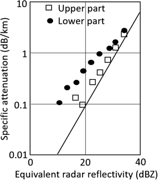
From the profiles of k and Z_e, coefficients, α and β, in the power low relationship as   

were determined. As the coefficients significantly varied according to relative height in the melting layer, the melting layer was divided into upper and lower parts. The upper part was from the Z_e peak point (B in Fig. 11) to the upper maximum slope point (A in Fig. 11), and the lower part was from the lower maximum slope point (C in Fig. 11) up to the Z_e peak point. The data of k and Z_e in the parts were classified every 3 dBZ in Z_e. Then k was averaged to obtain a relationship between averaged k and averaged Z_e (Fig. 14). The averaged k-Z_e relationship from Parsivel data in rain cases is also shown by a solid line in the figure. k for melting snow is greater than that of rain with the same Z_e. The scattergram seems different from Fig. 13. This is because of large scatter of data and variation of reference points. After the least square fitting to the data, which were greater than 0 dBZ, the coefficient α and β were obtained. The coefficients α and β were 0.0153 and 0.697 for the upper part, and 0.00393 and 0.772 for the lower part. Note that the number of cases were limited and the coefficients varied significantly.

Fig. 14.

Scattergram of averaged k and Z_e for 1 and 2 March, 2015. Black squares are for upper part of the melting layer, and open squares are for lower part of the melting layer. The solid line is for rain cases from Parsivel data.

4.5 Ground effect

The observation sites were located in a mountainous region, and the radar beam was separated from the ground by only ∼ 200 m. The snow particles were easily blown by winds, and their distribution might be easily affected by local wind variations induced by the topography. The two radar beams were slightly deviated from each other and the beam width was as narrow as 0.5°. Thus, the snow signatures measured by the two radars could easily be different from each other, particularly when the snow was light. Figure 15 shows an example. The specific attenuation shows large variations and sometimes negative specific attenuation, which is physically impossible. When the precipitation is heavy, such phenomena do not appear. As the estimated specific attenuation is sensitive to the profile difference, only rather heavy precipitation cases were used.

Fig. 15.

The same as Fig. 6, but a bad case at 02:00 JST on 14 November 2014.

The mountainous environment may also cause rapid variation in short time. Figure 16 shows the profiles at 07:07 JST and 07:08 JST on 14 November. Only 1-min temporal difference causes significant difference, particularly in k profiles and k-Z_e diagrams.

Fig. 16.

Profiles of equivalent radar reflectivity (a, d), specific attenuation (b, e), and k-Z_e diagram (c, f) at 07:07 (a, b, c) and 07:08 JST (d, e, f) on 14 November 2014.

Another thing to be considered is small liquid particles which contribute to specific attenuation. When a melting layer appears, small liquid particles may exist above the melting layer as dense fog. In fact, attenuation was sometimes detected from reduction of ground clutter, even though precipitation echo was not detected. Figure 17 shows a profile at 19:50 JST, 13 November. Specific attenuation increased slightly with height, even though precipitation echo weakened.

Fig. 17.

Profiles of equivalent radar reflectivity (a), specific attenuation (b), and k-Z_e diagram (c) at 19:50 JST, 13 November.

5. Simple model interpretation

The k-Z_e relationship in the melting layer shows a loop-shape, i.e., after melting starts, specific attenuation increases followed by equivalent radar reflectivity. Here, model results are presented showing that the loop-shape characteristic is robust.

There exist several models for melting snow particles. A typical one is a homogeneous sphere with a mixture of air, water, and ice. One of others is a sphere with an ice core and the water shell. The scattering cross sections can be calculated according to the Mie theory for the sphere model, or an extension of the Mie theory for the shell and sphere model (Aden and Kerker 1951).

Here, the simple homogenous sphere model is applied. In the homogeneous sphere model, part of the original ice and air mixture melts to water, air removes the particle, and then the particle shrinks. When the melting ratio which is the ratio of water mass to total mass is given, the relative permittivity ε is assumed as   

where f_w, f_i, and f_a are volume ratio of water, ice, and air of the particle, respectively. Defining the permittivity of snow, ε_s, as   

where f_si and f_sa are the volume ratios of ice and air in the original snow, Eq. (6) can be rewritten as   

where f_s is the volume ratio of snow in the water-snow mixture. Though several sophisticated permittivities of melting snow particles have been proposed and discussed (e.g., Meneghini and Liao 1996, 2000; Liao et al. 2009) including the well-known Maxwell-Garnett and Gruggeman permittivities (Markel 2016), the true permittivity is still uncertain, because of the complexity of the melting snow particles. Almost all the reported results show that the real part of the permittivity monotonically varies from ∼ 1 to some value, for example, 10 for a 35 GHz radiowave, with melting. The imaginary portion decreases from 0 to approximately −20 with melting. Because our purpose is to discuss qualitative characteristics of the k-Z_e relationship, Eq. (8) may be enough.

The complex refractive index (square root of permittivity) of ice is assumed to be fixed to (1.78–j0.0024). The complex refractive index for water depends on temperature and wavelength and is calculated from Ray's formula (Ray 1972) as (4.01–j 2.43) at 35.5 GHz and 0°C. During melting, the temperature of the particle is assumed 0°C. The density of the original snow is assumed to be 0.2 g cm⁻³. The mass melting ratio roughly corresponds to the downward length from the top of the melting layer. Figure 18 shows the backscattering cross sections, σ_b, scattering cross section, σ_s, absorption cross section, σ_s, and extinction cross section, σ_e, as functions of the mass melting ratios for a melted diameter of 1 mm. Figure 19 is the same but for a melted diameter of 2 mm. All curves have peaks during melting, but at different melting ratios. The peak of the extinction cross section, which relates to the specific attenuation, is at a smaller melting ratio than the backscattering cross section, which relates to the equivalent radar reflectivity. For a smaller particle, the extinction cross section is determined by the absorption cross section; however, for a larger particle, the portion of the scattering cross section in the extinction cross section becomes greater. The difference of peak positions for backscattering cross sections and extinction cross section is greater for larger particles. Heavy precipitation contains a great number of large particles resulting in a wide melting layer. This means that the height difference between the height of the attenuation peak and that of radar reflectivity is greater for heavier precipitation.

Fig. 18.

Cross sections as functions of mass melting rate for a melting particle with a melted diameter of 1 mm at 35.5 GHz. σ_s, σ_b, σ_a, and σ_e are scattering cross section, backscattering cross section, absorption cross section, and extinction cross section, respectively.

Fig. 19.

The same as Fig. 18, but with a diameter of 2 mm. The scales are different from Fig. 18.

What causes the changes of the scattering cross sections? Shapes of all particles are assumed spherical. Changes of the size and the permittivity depend on the mixing ratios of water, ice, and air. First, think of a Rayleigh scattering case. The Rayleigh scattering can be applied to cases wherein the size of the scatterer is much smaller than the wavelength of the radiowaves. The cases include precipitation observations by S, C, or X-band radars but are limited for Ka-band radar cases. The cross sections of Rayleigh scattering depend only on the wavelength λ, particle size D, and coefficient K [= (ε − 1)/(ε + 2)], and are written as:   

  

  

  

If the size is constant, the cross sections at a fixed wavelength depends only on the relative permittivity through K. Figure 20 shows the relationship between Im (−K) and |K²| of a melting snow particle, including a 10 GHz case for comparison. The complex refractive index of rain at 10 GHz is assumed to be (7.08 − j 2.87) where j is an imaginary unit. The left side of small |K²| corresponds to snow, whereas the right corresponds to rain. As melting starts, Im (−K) increases rapidly and then, | K² | increases. Im (−K) has more variation for 35 GHz compared with that for 10 GHz because of the difference of permittivity of water, which depends on the frequency. By substituting ρ_w = 1 and ε_a = 1 into Eq. (6), and by defining ε = ε′ + jε″, we have   

where m is the mass melting ratio. |K²| and Im (−K) are   

  

Above equations show that as the process of melting goes on (m increases from zero), | K²| monotonically approaches the value of 1. As for Im (−K), as melting goes on, noting that ε″ is negative, first the dividend dominates, and later the divider dominates, resulting in Im (−K) increase and then decrease.

Fig. 20.

Relationship between Im (−K) and |K²| of melting snow particle at 10 GHz and 35 GHz. The left (right) side corresponds to snow (rain).

Figure 21 shows the extinction cross sections of a melting snow particle as functions of the backscattering cross section in dB. Three curves correspond to (a) Rayleigh calculation with permittivity change and a fixed diameter of 1 mm, (b) Rayleigh calculation with permittivity and size change to a melted diameter of 1 mm, and (c) Mie calculation with permittivity and size change. Curve (a) shows only the permittivity effect and is the same as Fig. 20 except that the abscissa is in dB. Curve (b) shows the permittivity and size effects. The difference from (a) is due to the particle size change from a dry snow particle to a rain drop. The size of the snow particle depends on the density. Taking an original snow density of 0.2 g cm⁻³, the size is ∼ 1.7 times greater than the water equivalent particle size. Thus, the absorption cross section and scattering cross section are 5 times and 25 times greater than the water size particles. Curve (c) in the figure shows the result of the Mie calculation. The backscattering cross section of the Mie calculation is smaller than that of the Rayleigh calculation. By contrast, the extinction cross section of the Mie calculation is slightly greater than that of the Rayleigh calculation. The top point corresponds to the peak point of k, and the rightmost point corresponds to that of Z_e, meaning that the peak point of k is above that of Z_e.

Fig. 21.

The relationship between the extinction cross section, σ_e, and backscattering cross section, σ_b, for a melting snow particle with a diameter of 1 mm at 35.5 GHz. (a): Rayleigh calculation with a fixed diameter and permittivity change, (b): Rayleigh calculation with size change and permittivity change, and (c): Mie calculation. The arrows indicate the melting from snow to rain.

Figure 22 shows the same as Fig. 21, but the diameter of the melted particle is 2 mm. The difference between the curves (b) and (c) is more significant compared with that for the particle with the 1 mm diameter. The difference is attributed to the difference in the backscattering cross section. The Mie scattering effect suppresses the backscattering cross sections from Rayleigh scattering. Another difference to be noticed is that the difference of the backscattering cross sections at its maximum and at the rain drop is smaller. This fact is also presented in Figs. 18 and 19, suggesting that this is the cause of the shelf-like profile instead of the peak-type profile of the bright band at the Ka-band due to the Mie effect.

Fig. 22.

The same as Fig. 21, but with a diameter of 2 mm. The scales are different from Fig. 21.

Figures 21 and 22 show that the basic loop-shape is due to the change in permittivities. This characteristic appears similar even when Maxwell-Garnett or Gruggeman permittivities (not shown) are applied.

When a radiowave frequency is S-, C-, or X-band, σ_e is much greater than σ_s, and the extinction cross section is determined by the absorption cross section. For the higher frequency, such as the Ka-band, the deviation from the Rayleigh scattering becomes significant. When the scattering cross section becomes comparable with the absorption cross section, it results in a complicated k-Z_e relationship.

Although the results shown above are only for two drop sizes, they show basic mechanism of the loopshape characteristics in the k-Z_e diagram. More realistic simulation should take the drop size distribution into consideration.

6. Conclusion

Specific attenuation and equivalent radar reflectivity in a melting layer were measured using a dual Ka-band radar system. The system consists of two identically designed Ka-radars. When a precipitation system came between the two radar sites, the radars observed the system from opposite directions. The precipitation echoes suffered from rain attenuation. The reduction due to rain attenuation symmetrically appears in both radar echoes. By differentiating the averaged measured radar reflectivity with the range, the specific attenuation (k) can be estimated. After obtaining the specific attenuation, the equivalent radar reflectivity (Z_e) is estimated. In the melting layer, specific attenuation and the equivalent radar reflectivity varied significantly along the radio path. The relationship showed interesting characteristics, i.e., a loop-shape on the k-Z_e diagram. The reasons for the loop-shape are: (1) changes in relative permittivity, (2) changes of particle sizes, and (3) the Mie effect. Therefore, the scattering characteristics can be understood with separate causes. However, the particles are assumed spherical in the current analysis, and this assumption should be investigated with more sophisticated models (e.g., Johnson et al. 2016; Leinonen and von Leber 2018).

The observational results could contribute to improvement of the DPR rain retrieval algorithms, particularly for melting snow or wet snow. At present, there are several models for the melting layer, and the results here may contribute to the model reliability. Uncertainty of the estimation of the accuracy of the equivalent radar reflectivity and specific attenuation still persist, and the observation locations may limit applicability of the results. The observation locations were on mountain slopes. The radio path of the radar was separated from the ground by approximately only ∼ 200 m, and although the ground clutter did not contaminate the radar signature thanks to the narrow beam and well suppressed far sidelobes in the antenna pattern, the conditions may have been different from the free atmosphere. For example, slope winds may have deformed the structure of the melting layer.

Acknowledgments

The authors would like to thank Toshio Iguchi from NICT for many valuable comments throughout our research. The DKR was built by Mitsubishi Electric Tokki Systems Corporation (Japan). Michinobu Nonaka, Hydrotech Co. Ltd. assisted with the observations. Much research in the field has been done by Masanori Nishikawa from Hokkaido University. This research was supported by JAXA as the 7th and 8th Research Announcements activities. The authors would also like to thank the anonymous reviewers for their valuable comments, and Editage (https://www.editage.jp) for English language editing.

References

•  Aden,  A. L., and  M.  Kerker, 1951: Scattering of electromagnetic waves from two concentric spheres. J. Appl. Phys., 22, 1242, doi:10.1063/1.1699834.
•  Fabry,  F., and  I.  Zawadzki, 1995: Long-term radar observations of the melting layer of precipitation and their interpretation. J. Atmos. Sci., 52, 838-851.
•  Hou,  A. Y.,  R. K.  Kakar,  S.  Neeck,  A. A.  Azarbarzin,  C. D.  Kummerow,  M.  Kojima,  R.  Oki,  K.  Nakamura, and  T.  Iguchi, 2014: The global precipitation measurement mission. Bull. Amer. Meteor. Soc., 95, 701-722.
•  Johnson,  B. T.,  W. S.  Olson, and  G.  Skofronick-Jackson, 2016: The microwave properties of simulated melting precipitation particles: Sensitivity to initial melting. Atmos. Meas. Tech., 9, 9-21.
•  Kobayashi,  T.,  M.  Nomura,  A.  Adachi,  S.  Sugimoto,  N.  Takahashi, and  H.  Hirakuchi, 2021: Retrieval of attenuation profiles from the GPM dual-frequency radar observations. J. Meteor. Soc. Japan, 99, 621-648.
•  Kollias,  P., and  B.  Albrecht, 2005: Why the melting layer radar reflectivity is not bright at 94 GHz? Geophys. Res. Lett., 32, L24818, doi:10.1029/2005GL024074.
•  Leary,  C. A., and  R. A.  Houze, Jr., 1979: Melting and evaporation of hydrometeors in precipitation from the anvil clouds of deep tropical convection. J. Atmos. Sci., 36, 669-679.
•  Leinonen,  J., and  A.  von Leber, 2018: Snowflake melting simulation using smoothed particle hydrodynamics. J. Geophys. Res.: Atmos., 123, 1811-1825.
•  Li,  H., and  D.  Moisseev, 2019: Melting layer attenuation at Ka- and W-bands as derived from multi-frequency radar Doppler spectra observations. J. Geophys. Res.: Atmos., 124, 9520-9533.
•  Li,  L.,  S. M.  Sekelsky,  S. C.  Reising,  C. T.  Swift,  S. L.  Durden,  G. A.  Sadowy,  S. J.  Dinardo,  F. K.  Li,  A.  Huffman,  G.  Stephens,  D. M.  Babb, and  H. W.  Rosenberger, 2001: Retrieval of atmospheric attenuation using combined ground-based and airborne 95-GHz cloud radar measurements. J. Atmos. Oceanic Technol., 18 1345-1353.
•  Liao,  L.,  R.  Meneghini,  L.  Tian, and  G. M.  Heymsfield, 2009: Measurements and simulations of nadir-viewing radar returns from the melting layer at X and W bands. J. Appl. Meteor. Climatol., 48, 2215-2226.
•  Markel,  V. A., 2016: Introduction to the Maxwell-Garnett approximation: Tutorial. J. Opt. Soc. Amer., 33, 1244-1256.
•  Marshall,  J. S., and  W.  Mc K. Palmer, 1948: The distribution of raindrops with size. J. Meteor., 5, 165-166.
•  Meneghini,  R., and  L.  Liao, 1996: Comparisons of cross sections for melting hydrometeors as derived from dielectric mixing formulas and a numerical method. J. Appl. Meteor., 35, 1658-1670.
•  Meneghini,  R., and  L.  Liao, 2000: Effective dielectric constants of mixed-phase hydrometeors. J. Atmos. Oceanic Technol., 17, 628-640.
•  Minda,  H.,  T.  Makino,  N.  Tsuda, and  Y.  Kaneko, 2016: Performance of a laser disdrometer with hydrometeor imaging capabilities and fall velocity estimates for snowfall. IEEJ Trans. Electrical Electronic Eng., 11, 624-632.
•  Nakamura,  K., 2021: Progress from TRMM to GPM. J. Meteor. Soc. Japan, 99, 697-729.
•  Nakamura,  K.,  S.  Shimizu,  K.  Nakagawa, and  H.  Hanado, 2011: Dual Ka-band radar experiment for the DPR algorithm development. Proceeding of the IEEE International Geoscience And Remote Sensing Symposium, Vancouver, Canada, 1554-1557.
•  Nakamura,  K.,  Y.  Kaneko,  K.  Nakagawa,  H.  Hanado, and  M.  Nishikawa, 2018: Measurement method for specific attenuation in the melting layer using a dual Ka-band radar system. IEEE Trans. Geosci. Remote Sens., 56, 3511-3519.
•  Nishikawa,  M.,  K.  Nakamura,  Y.  Fujiyoshi,  K.  Nakagawa,  H.  Hanado,  H.  Minda,  S.  Nakai,  T.  Kumakura, and  R.  Oki, 2016: Radar attenuation and reflectivity measurements of snow with dual Ka-band radar. IEEE Trans. Geosci. Remote Sens., 54, 714-722.
•  Olsen,  R.,  D.  Rogers, and  D.  Hodge, 1978: The aR^b relation in the calculation of rain attenuation. IEEE Trans. Antennas Propag., 26, 318-329.
•  Ray,  P. S., 1972: Broadband complex refractive indices of ice and water. Appl. Opt., 11, 1836-1844.
•  Seto,  S.,  T.  Iguchi,  R.  Meneghini,  J.  Awaka,  T.  Kubota,  T.  Masaki, and  N.  Takahashi, 2021: The precipitation rate retrieval algorithms for the GPM Dual-frequency Precipitation Radar. J. Meteor. Soc. Japan, 99, 205-237.
•  Suzuki,  K.,  R.  Kamamoto,  K.  Nakagawa,  M.  Nonaka,  T.  Shinoda,  T.  Ohigashi,  Y.  Minami,  M.  Kubo, and  Y.  Kaneko, 2019: Ground validation of GPM DPR precipitation type classification algorithm by precipitation particle measurements in winter. SOLA, 15, 94-98.