Application of a Nudged General Circulation Model to the Interpretation of the Mean Age of Air Derived from Stratospheric Samples in the Tropics

Abstract

Stratospheric profiles of the mean age of air estimated from cryogenic air samples acquired during a field campaign over Indonesia, the Coordinated Upper-Troposphere-to-Stratosphere Balloon Experiment in Biak, were investigated using the boundary impulse evolving response (BIER) method and Lagrangian backward trajectories, with the aid of an atmospheric general circulation model-based chemistry transport model (ACTM). The ACTM provides realistic meteorological fields at 1-hour intervals by nudging toward the European Centre for Medium- Range Weather Forecasts Reanalysis-Interim. Since the BIER method is capable of taking unresolved diffusive processes into account, while the Lagrangian method can distinguish the pathways the air parcels took before reaching the sample site, the application of the two methods to the common transport field simulated by the ACTM is useful in assessing the CO₂- and SF₆-derived mean ages. The reliability of the simulated transport field has been verified by the reproducibility of the observed CO₂, SF₆, and water vapor profiles using the Lagrangian method. The profile of CO₂ age is reproduced reasonably well by the Lagrangian method with a small young bias being consistent with the termination of trajectories in finite length of time, whereas the BIER method overestimates the CO₂ age above the altitude of 25 km, possibly due to high diffusivity in the transport model. In contrast, the SF₆ age is only reproducible in the lower stratosphere, and far exceeds the estimates from the Lagrangian method above the altitude of 25 km. As air parcels of mesospheric origin are excluded in the Lagrangian age estimation, this discrepancy, together with the fact that the observed SF₆ mole fractions are much lower than the trajectory-derived values in this height region, supports the idea that the stratospheric air samples are mixed with SF₆-depleted mesospheric air, leading to overestimation of the mean age.

1. Introduction

The tropical atmosphere is characterized by the highest and coldest tropopause, as well as warm and humid air in the lower troposphere. In a study of stratospheric dryness, Brewer (1949) noted these features as the key to understanding the global-scale stratospheric circulation. His water vapor observations, along with the interpretation of the global ozone distributions by Dobson (1956), led to the conclusion that the tropospheric air enters the stratosphere primarily through the cold tropical tropopause and spreads toward high latitudes. This Brewer–Dobson circulation (BDC) constitutes the basis of the dynamics as well as tracer transport in the stratosphere.

The response of the BDC to natural and anthropogenic forcings is one of the primary issues of current stratospheric research (Butchart 2014; Hasebe et al. 2018, hereafter referred to as H18). Modulation of the BDC, such as changes in the velocities, mass transport and pathways of circulation, is often diagnosed by using stratospheric age of air (AoA), originally defined as the length of time elapsed since the air parcel entered the stratosphere (Kida 1983). The AoA can be intuitively understood as the time lag of the concentration growth of “clock tracers” between the troposphere and stratosphere. For example, successive observations of carbon dioxide (CO₂) and sulfur hexafluoride (SF₆), given their anthropogenically driven increase and chemically conservative nature, make it possible to use their stratospheric value as a time stamp of their entry into the stratosphere. As such, the delay of the time-series in the stratosphere relative to that in the troposphere could be a measure of the mean age (Elkins et al. 1996; Boering et al. 1996; Harnisch et al. 1996; Patra et al. 1997; Andrews et al. 2001b). Accumulated observations of CO₂ and SF₆ mole fractions in the northern midlatitude stratosphere (e.g., Schmidt et al. 1987; Nakazawa et al. 1995; Engel et al. 2002) have been used to estimate the long-term trend of mean age after careful consideration of the nonlinearity in the growth of these species. The results show an increase (though not statistically significant) at a rate of 0.24 ± 0.22 years decade⁻¹ (Engel et al. 2009). Although this rate has been reduced to 0.15 ± 0.18 years decade⁻¹ as per a recent study (Engel et al. 2017), these estimates are still apart from the long-term decrease of mean age diagnosed by chemistry-climate models (e.g., Austin et al. 2007; Garcia et al. 2011). For example, Garcia et al. (2011) showed that the AoA trend derived from SF₆ during the period 1965–2006 by the Whole Atmosphere Community Climate Model (WACCM) is −0.086 ± 0.011 years decade⁻¹. Efforts are being made to resolve this disagreement by reducing uncertainties in both the observational and model estimates, such as those arising from limited observational data of seasonally varying CO₂ mole fractions and unavoidable use of parameterization schemes associated with a coarse model resolution (e.g., Garcia et al. 2011; Stiller et al. 2012; Diallo et al. 2012).

Any air mass is composed of a large number of air parcels, each with a different transport pathway and transit time. Such multiple pathways taken by the air parcels pose a fundamental difficulty in interpreting the mean age. A complete description of the age of a given air mass is thus captured by the age spectrum, which is a statistical distribution of the parcel transit times (Kida 1983; Hall and Plumb 1994; Waugh and Hall 2002). Although an age spectrum is not directly observable, model simulations indicate that it has a long tail in the midlatitude stratosphere, which increases the mean age appreciably. Given that the tropospheric air enters the stratosphere primarily in the tropics and that the air parcels inside the “tropical leaky pipe” are relatively isolated from mid- and high latitudes by the subtropical mixing barrier (Plumb 1996; Neu and Plumb 1999), the mean age is relatively young in the tropical lower stratosphere and the age spectrum takes a compact shape due to transport by slow diabatic advection and very low contributions from the subtropical mixing and diffusion (Plumb and Eluszkiewicz 1999). The tropical stratosphere is also unique in that the ascending motion is visualized by the water vapor “tape recorder” (Mote et al. 1996). This is independent of mean age because it is an imprint of seasonally varying tropopause temperature on the water vapor mixing ratio in the ascending air masses. All these features make the interpretation of the stratospheric mean age simpler in the tropics than the midlatitudes. In particular, the observations in the tropics are quite limited.

Motivated by these considerations, the Coordinated Upper-Troposphere-to-Stratosphere Balloon Experiment in Biak (CUBE/Biak), a field campaign over Indonesia, was conducted from February to March 2015 (H18). CUBE/Biak involved whole air sampling with the aid of balloon-borne cryogenic samplers; radiosondes equipped with ozone, water vapor, and CO₂ sondes; optical particle counters; cloud particle sensor; and aerosol samplers, along with the continuous operation of aerosol lidar on the ground.

The present study aims to assess the vertical profiles of AoA, estimated from the mole fractions of CO₂ and SF₆ obtained via cryogenic air sampling during the CUBE/Biak campaign (Sugawara et al. 2018, hereafter referred to as S18). The boundary impulse evolving response (BIER) method and Lagrangian backward trajectories are used for the estimation of the age spectra. In the former method, the stratospheric concentrations of trace gases are interpreted as the response to forcing in the source region (Hall and Plumb 1994; Waugh and Hall 2002). In contrast, the latter method constructs the age spectrum by tracing a large number of air parcels in a three-dimensional wind field by backward trajectories (Fueglistaler et al. 2005, H18). An atmospheric general circulation model (AGCM)-based chemistry transport model (ACTM), which is nudged to European Centre for Medium-Range Weather Forecasts Reanalysis - Interim (ERA-Interim; Dee et al. 2011) fields, is used for both methods. A concise introduction of the mathematical formulation of the age spectrum is given in Section 2. The observations and the model experiments, including the model evaluation and a brief review of the analysis methods, are described in Section 3. The application of the model experiments to the CUBE/Biak observations are presented in Section 4. Differences between the observationally and experimentally estimated mean ages are discussed in Section 5. Finally, a summary is given in Section 6.

2. Age spectrum and mean age of air

A mathematical formulation of the age spectrum was first presented by Hall and Plumb (1994). The tracer mixing ratio at a position r and time t, χ (r, t), is interpreted as a response to that at source region Ω at time t′, χ (Ω, t′):   

Here G (r, t | Ω, t′) is a Green's function that specifies the contributions from Ω at various past times t′ to the mixing ratio at (r, t) (Waugh and Hall 2002). By introducing the transit time τ ≡ t − t′, Eq. (1) reduces to   

Eq. (2) shows that G (r, t | Ω, t − τ) dτ is the mass fraction of air at (r, t) that had last been in contact with Ω between τ and τ + dτ ago. In other words, G (r, t | Ω, t − τ) specifies the distribution of elapsed time since stratospheric entry and is termed the age spectrum. In this sense, t and t′ are called the field time and source time, respectively. By definition, the mean age Γ is estimated as the first moment of the age spectrum:   

The spectral width (spread) is often measured by Δ, which is defined as follows:   

3. Data and method

3.1 Mean age estimation from air samples

The mole fractions of CO₂ and SF₆ derived from the air samples taken from the CUBE/Biak campaign are used to estimate the mean AoA. The overall uncertainties of the observed mole fractions are 0.1 µmol mol⁻¹ for CO₂ and better than 0.09 pmol mol⁻¹ for SF₆, leading to possible errors in the mean age of 0.3–0.4 years for CO₂ and 0.4–0.5 years for SF₆. See S18 for the details of the preprocessing of collected samples. For this estimation, the age spectrum, having been assumed to take the form of the inverse-Gaussian distribution (Waugh and Hall 2002),   

is sought to reproduce the observed mole fraction of the corresponding species by sweeping the parameter Γ. This function is known as the solution of the continuity equation for linearly increasing tracers in a one-dimensional diffusive system (Hall and Plumb 1994). While only one value (mole fraction) is known, the other parameter Δ is assumed to be given by Γ as per the relationship Δ²/Γ = 0.7 years. This value, called the ratio of moments, is suggested by Hall and Plumb (1994) from the results of a stratospheric AGCM and is found to give the best overall agreement between SF₆-derived and CO₂-derived mean ages in the northern mid- and high latitude stratosphere (Engel et al. 2002). Then the mole fraction at time t, derived by substituting Eq. (5) together with known tropospheric values χ₀ (t) into Eq. (2),   

is compared with observations, and the parameter Γ that gives the best match to the observation is adopted as the observational estimate of the mean age. In the CUBE/Biak campaign, the tropospheric reference was derived from direct measurements of air samples collected by the Comprehensive Observation Network for TRace gases by AIrLiner (CONTRAIL) program (Machida et al. 2008; Sawa et al. 2008; Matsueda et al. 2015) in the tropical upper troposphere within the area 5°S–5°N and 142–150°E at an altitude of 10–13 km (S18).

3.2 Mean age estimation from model experiments

The estimation of the mean age using the transport model ACTM relies on the age spectra derived by BIER and Lagrangian methods. The details are described below.

a. Description of the model and simulation design

The ACTM used in the present study was developed on the basis of the Center for Climate System Research/National Institute for Environmental Studies/Frontier Research Center for Global Change (CCSR/NIES/FRCGC) AGCM (Numaguti et al. 1997; Patra et al. 2009). It is configured as in Ishijima et al. (2010) to have 67 sigma levels from the surface to a height of ∼ 90 km with the horizontal resolution in T42 spectral truncation (equivalent to approximately 2.8° ´ 2.8° latitude–longitude gridpoints). The cumulus convection parameterization scheme is the simplified Arakawa and Schubert scheme (Arakawa and Schubert 1974; Numaguti et al. 1997). The adjusted cloud mass flux is used to calculate the updraft and downdraft due to cumulus convection. Gravity wave drag is calculated using a scheme of McFarlane (1987). Influence of gravity wave on the stratospheric circulation in this and newer version of ACTM was discussed in detail by Patra et al. (2018). For the calculation of tracer transport, it applies a fourth-order flux-form advection scheme using a monotonic Piecewise Parabolic Method (PPM) (Colella and Woodward 1984) and a flux-form semi-Lagrangian scheme (Lin and Rood 1996). The second-order vertical eddy diffusion scheme of Mellor and Yamada with cloud effects (Mellor and Yamada 1982; Numaguti et al. 1997) is applied for subgrid-scale vertical fluxes of meridional velocity, temperature, surface pressure, and mixing ratios of tracers. This model has been used in studies of the transport properties of chemical constituents such as nitrous oxide (N₂O) (Ishijima et al. 2010) and in demonstrating the utility of a novel three-dimensional transport formulation (Kinoshita et al. 2019).

The simulation has been conducted by nudging the horizontal winds and temperature toward those of the ERA-Interim with the relaxation time of 2.4 hours at 6-hour time intervals from 1 January 2000 to 31 March 2015. The choice of relatively strong nudging comes from our experience of ACTM simulations to better reproduce observed N₂O and its isotopic ratios in the stratosphere (Ishijima et al. 2015). Sea ice and sea-surface temperature (SST) fields are also supplied from the ERA-Interim at 6-hour time intervals. The first five years (January 2000 to December 2004) are regarded as the spin-up period and are excluded in the following analysis. For the ozone field for radiative calculations, 6-hourly full-resolution model level data up to 1 hPa from the ERA-Interim (Dragani 2011), and above 1 hPa from United Kingdom Universities' Global Atmospheric Modelling Programme (UGAMP) ozone climatology (Li and Shine 1999) are used. A supplementary free run, wherein nudging of horizontal winds and temperature to ERA-Interim is terminated after spinning up, is also made to see the effect of nudging on the transport features (Section 4.2).

For estimating the age spectra, artificial inert tracers are released in temporal “pulses” from the source region placed at the tropical surface corresponding to the latitude band 15°S–15°N by setting their mixing ratio to a constant value (1 ppbv) for a month (pulse tracers). The releases are made in odd-numbered months; i.e., January, March, May, July, September, and November of each year throughout the simulation period (January 2005 to March 2015), resulting in the release of 62 distinct tracers in total.

b. Evaluation of the model performance

Before moving on to the estimation of the age spectra, the performance of our ACTM was investigated by viewing the distribution of the aforementioned artificial tracers. The pulse-wise release of inert tracers from a single source region helps avoid the complexity in describing the transport field. The latitude–height distribution of the simulated pulse tracers were examined in the averaged distribution of tracers released in the same calendar month but in different years from 2005 to 2013. The Northern winter transport field was investigated as an example in the top panels of Fig. 1 by examining the zonal-mean distribution of January-released tracers in (a) February of the first year (i.e., the next month) and (b) February of the second year (i.e., 13th month since release).

Fig. 1.

Monthly mean distributions of surface-released pulse tracers (ppbv) during (a) February of the first year, and (b) February of the second year from release in January. The dotted yellow line is the tropopause position (defined by World Meteorological Organization). Area covered by the purple lines represents the TTL. White curves show the transformed Eulerian mean residual stream function (kg m⁻¹ s⁻¹). Evolution of January (red) and July (blue) BIRs on (c) 100, 50, and 10 hPa over the equator and (d) 50 hPa at 20.9, 46.0 and 79.5°N. The thick lines are the average of five BIRs for tracers released from 2005 to 2009, whereas the shading shows the BIR range among the five releases.

During the few months after release (Fig. 1a), tracers were transported by the tropospheric Hadley circulation from the source region and stayed mostly in the troposphere, except for some air entering the tropical tropopause layer (TTL) and the lower stratosphere (LS). The tropospheric tracers were trapped more in the winter hemisphere due to the deflection to the summer hemisphere of the ascending branch of the Hadley circulation. Stratospheric concentrations above the 400 K isentrope in the subtropics and in the lowermost stratosphere at mid- and high latitudes were higher in the winter hemisphere than in the summer hemisphere, suggesting a stronger circulation toward the winter pole. One year later (Fig. 1b), the surface-released tracers had been transported into the stratosphere. A tropical maximum at ∼ 500 K isentrope (∼ 50 hPa) indicates that a part of the tracers that were widespread in the TTL one year earlier had been pumped up into the tropical stratosphere. At the same time, some tracers, having leaked from the tropical pipe, were transported to the extratropics by quasi-isentropic mixing to create lower-stratospheric maxima in mid- and high latitudes. The altitude and sharpness of the maximum reflect the strength of the extratropical suction pump and permeability of the subtropical mixing barrier. The lower-stratospheric maxima, having a value of > 0.12 ppbv in the mid- and high latitudes, were found at higher isentropic levels in the Southern Hemisphere, as a result of the seasonal and hemispheric anisotropy of both the shallow and deep branches of the BDC.

The transport features described above are limited to those at a specific time in the Northern winter. The temporal evolutions of a single pulse tracer at some representative altitudes and latitudes are shown in the bottom panels of Fig. 1 in the form of time series called the boundary impulse responses (BIRs) (Li et al. 2012a; Ploeger and Birner 2016). Here the values are scaled so that they express the probability distribution function (PDF) to be used in the mean age estimation (Section 3.2c). Curves in red and blue show those released in January and July, respectively. Because the coverage of our transport calculation is limited to ∼ 10 years from January 2005 to March 2015, we show the five-year time-series of tracers by taking the average of those released in January (red) and July (blue) of 2005, 2006, 2007, 2008, and 2009. Panel (c) shows the PDF over the equator (the average of two BIRs at 1.4°N and 1.4°S) at 100, 50, and 10 hPa pressure levels, and panel (d) illustrates that at latitudes 20.9, 46.0, and 79.5°N at 50 hPa. The shading surrounding the thick lines are the five-year range between the maxima and minima. In the tropics, the BIR-peaks appear earlier and higher for the tracers released in January than in July at 100 hPa. However, this is not always the case for the 50 hPa and 10 hPa levels. Upon the passage of westerly (easterly) wind shear associated with the quasi-biennial oscillation (QBO) in the LS below these levels, the accompanying descending (ascending) motion will bring about later (earlier) BIR peaks [see Ploeger and Birner (2016)]. The BIR at 50 hPa over the equator reaches a maximum several months after release. At 10 hPa, the transit time of ∼ 2 years necessary for the surface tracers to reach a maximum is concurrent with that observed by Li et al. (2012b) [see their Fig. 1 (top)], although the decay time appears longer in the present study. Sufficient mixing and recirculation occurs higher up at 10 hPa. Rapid isentropic mixing explains part of the widening of the age spectrum, explaining contributions from air parcels with large transit times due to back and forth recirculation between the tropical pipe and the midlatitudes. The latitudinal variation of the BIRs at 50 hPa shows a tendency for peaks to be later and smaller and the decay time to be longer at higher latitudes. The seasonal dependency of our results at 20.9°N at 50 hPa agrees with that at 20°N on the 420 K isentrope (∼ 70 hPa) found by Li et al. (2012a). That is, the January-BIR shows an earlier and higher peak than the July-BIR. These results are concurrent with previous studies and with current knowledge, indicating that the AGCM realistically time-interpolates the discrete ERA-Interim wind data and simulates dynamical–physical processes of tracer transport reasonably well.

c. Estimation of the age spectra by BIER method

The age spectrum is a boundary propagator G (r, t | Ω, t − τ) introduced in the form of a Green's function (Section 2). It could be estimated from the response χ (r, t) by setting the tracer mixing ratio at the source region as a “pulse” at τ = τ_i (≥ 0), i.e., by substituting the Dirac delta function δ (τ − τ_i) for χ (Ω, t − τ) in Eq. (2):   

Equation (7) can be interpreted as a function of τ_i (≥ 0) for a fixed (r, t), and χ (r, t) is referred to as the BIR (Haine et al. 2008; Li et al. 2012a). In practice, δ (τ − τ_i) is approximated by the mixing ratio of an inert pulse tracer χ (Ω, t − τ _i) released at the source region Ω at the source time t − τ _i. The principle of this method is schematically illustrated in Fig. 2a.

Fig. 2.

Schematic illustration of the concept of the age spectrum at a location r and time t calculated using (a) Boundary Impulse Evolving Response (BIER) and (b) Lagrangian backward trajectory methods. Thick yellow lines show the subtropical mixing barriers. Hatched area shows the tropical tropopause layer (TTL). Purple area depicts the location of CONTRAIL observations used as the upper tropospheric reference record. χ (r, t) is the mixing ratio at (r, t). χ (Ω, t − τ_i) is the mixing ratio at the source region Ω (shaded area) at the source time t − τ_i. Dashed arrows illustrate the propagation from the source region to stratospheric air parcel by the boundary propagator G (r, t | Ω, t − τ_i) in the BIER method. Solid wavy arrows are the trajectories in the Lagrangian method, wherein the count of transit time commences with the last passage through 355 K isentrope. LCP is the Lagrangian cold point defined as the coldest point along each trajectory. The insets represent the shape of the age spectrum at (r, t).

This method was modified by implementing multiple pulse tracers with different source time t − τ _i in a single transport calculation (BIER method) making it possible to estimate the time-dependent age spectrum efficiently (Ploeger and Birner 2016). In our experiment, 62 one-month pulses are introduced as χ (Ω, t − τ_i) (Section 3.2a), creating 62 BIRs. These BIRs will build a BIR map for a point r with horizontal and vertical axes corresponding to the source time and field time, respectively. The age spectrum at r is the horizontal cut of the BIR map backward in source time at the field time t. As the transport calculations cannot last for an infinite length of time, the integration must be truncated at some finite length, which leads to errors in the age estimation. To overcome this, a tail correction has been applied in previous studies (e.g., Hall et al. 1999; Reithmeier et al. 2008; Li et al. 2012a; Ploeger and Birner 2016). Following Ploeger and Birner (2016), an exponential function was fitted to each age spectrum derived from the transport calculations and the obtained decay rate was used to extrapolate the age spectrum to infinity. The mean age derived by applying the tail correction to the truncated age spectra is denoted by Γ_corr in the present study.

The latitude–height section of the seasonal mean Γ_corr is shown in Fig. 3 with the potential temperature as the vertical coordinate. As our simulation design, the method of tail correction, and the use of ERA-Interim meteorological fields mostly follow those of Ploeger and Birner (2016), it is possible to compare our Fig. 3 with their Fig. 4. There is good consistency regarding overall features including the seasonal asymmetry between the hemispheres, strong latitudinal gradient associated with the subtropical mixing barriers, small slope of contours in high-latitude LS in the summer hemisphere, and so on. However, there are some quantitative differences at high latitudes. In the case of the December–January–February (DJF) average, for example, the 4.5-year contour lies above the 650 K and 500 K surfaces at 90°S and 90°N, respectively, in Fig. 3, whereas it lies below 500 K and 450 K, respectively, in Ploeger and Birner (2016), indicating that the mean age is younger by approximately 0.5–1.0 year in our ACTM. The younger age also appears in the June–July–August (JJA) average over Antarctica. This tendency is recognized from the AoA intercomparison of global transport models; the ACTM nudged to Japanese 25-year Reanalysis (JRA-25; Onogi et al. 2007) horizontal winds and temperature showed the strongest convective mixing in the tropics and the youngest air at the high-altitude poles among the models that participated in the comparison (Krol et al. 2018). These features that suggest an overall underestimation of the mean age in mid-to-high latitudes are thought to arise mostly from slightly too diffusive vertical transport of the ACTM (Patra et al. 2018). Despite the availability for only 3 years (2012–2014) for estimating the multiyear age spectra, the overall consistency is encouraging.

Fig. 3.

Zonal-mean distribution of three-year averaged mean age in the Northern Hemisphere winter (DJF) and summer (JJA) obtained using the BIER method. The potential temperature (K) is taken as the vertical coordinate.

Fig. 4.

Age spectra estimated using the (a) BIER method and (b) Lagrangian method corresponding to the altitudes of eight cryogenic air samples acquired during CUBE/Biak 2015. The temporal resolution is two months in both panels.

d. Estimation of the age spectra by Lagrangian method

The age spectra in the Lagrangian method are estimated, independently from the BIER method but relying commonly on the ACTM transport field, by counting the transit time τ during the advection along each kinematic trajectory since the last passage through the top of the troposphere (Tr_top) (Fig. 2b). In the present analysis, T_rtop is taken to be the 355 K isentropic surface referring to the fact that the influence of tropical convective motion almost ceases at this level and diabatic forcing gradually changes to radiative heating in and above the TTL (Hasebe and Noguchi 2016). Calculations are terminated when the trajectories reach the bottom (ground surface) and the top (1 hPa pressure level) boundaries. The trajectory calculations thus conducted could be applied to reconstructions of stratospheric concentrations of water vapor by assuming that the air parcel retains the saturation water mixing ratio (SMR) that takes a minimum (SMR_min) at the coldest point along each trajectory from the troposphere to the stratosphere (the Lagrangian cold point; LCP) (e.g., Bonazzola and Haynes 2004; Fueglistaler et al. 2005; Hasebe and Noguchi 2016). Likewise, stratospheric CO₂ and SF₆ concentrations are estimated by assuming that the air parcel conserves the mole fractions of these species at the time of the last passage through Tr_top. These values are set by referring to the CONTRAIL data compiled by S18 (Section 3.1) considering the rapid uplift of air in the tropical troposphere. By comparing these values with observations, the validity of the trajectory calculation could be investigated, which is useful for examining the reliability of the obtained age spectra and mean age.

The model parameters for calculating the kinematic backward trajectories are summarized in Table 1, and are compared with those from our previous attempt (H18). Pressure levels of the ACTM additional to those of the ERA-Interim in the TTL help to better resolve the LCP, which is critical for the precise estimation of the “tape recorder” profile. The present study tries to resolve disagreements between the estimates from trajectory calculations and the observations from CUBE/Biak by increasing the number of trajectories and extending the integration period (Table 1). Improvements are not limited to these simulation settings. In addition to using the ERA-Interim analysis directly as 6-hour interval snapshots, the assimilated meteorological field created by nudging its horizontal winds and temperature to the ACTM are also used for trajectory calculations. In this case, 1-hour averaged values are used at 1-hour intervals (ACTM-NUDG).

4. Application to CUBE/Biak observations

The vertical profiles of CO₂ and SF₆ ages estimated from the CUBE/Biak air samples by S18 are investigated by employing the BIER method and Lagrangian backward trajectories in this section. Both methods take account of the interannual as well as annual variations of meteorological field, making it possible to compare with the results from CUBE/Biak field campaign; however, possible deviations of March 2015 from climatological March cannot be ruled out.

4.1 BIER method

The age spectra corresponding to CUBE/Biak cryogenic air samples are shown in Fig. 4a. A unimodal distribution (∼ 0.3 years) and a rapid decrease (after ∼ 1 year) can be observed at some levels above the top of the TTL. Multimodal distributions with a long tail, caused by combination of annual cycle in upwelling and horizontal mixing between the extratropics and tropics, are found above 24 km. The long spectral tail considerably affects the magnitude of the mean age (Schoeberl et al. 2005; Li et al. 2012b). These age spectra are used to estimate not only Γ_corr, but also the spread of the transit times (Δ) (Hall and Plumb 1994; Waugh and Hall 2002). Calculations were extended to other latitudes and heights to construct the meridional section of Γ_corr in March 2015 (Fig. 5). The deformation of the contours at 3.0, 3.5, and 4.0 years, showing wavy structures in the tropics are due to the downward motion associated with the westerly shear of the QBO. The capability to estimate non-stationary age spectra for complete three-dimensional transport, including mixing, is one of the advantages of the BIER method (Ploeger and Birner 2016).

Fig. 5.

Latitude–height section of the mean age in March 2015 estimated using the BIER method using tracers released from January 2005 to March 2015 at the tropical surface (15°S–15°N). The age correction is applied using the transit time from the 4th to 10th years. The 355 K and 400 K isentropes are shown as white lines bounded between 30°N and 30°S indicating the location of Tr_top and the top of the TTL, respectively.

The values of Γ_corr shown in Fig. 5 are derived by taking Ω at the tropical surface. In contrast, the observational estimates of the mean age by S18 refer to the tracer concentrations in the tropical upper troposphere. Therefore, it is necessary to address the difference in the definition of the reference time from which age counting is started before making direct comparison between the two. As is evident from Fig. 1, the excursion of the tropospheric air to the stratosphere depends on tropospheric transport features, including isentropic mixing with the air in the extratropical LS, and thus the mean age counted from the tropical surface is not always a sum of the tropospheric residence time and the mean age counted from the TTL. Unfortunately, BIER calculations assigning Ω to the TTL are confronted with an alternative difficulty, i.e., the assumption that considers the TTL as a single source region appears inappropriate due to its wide coverage in latitude and height. In the present analysis, we use the adjusted mean age defined by subtracting the transit time at Tr_top from Γ_corr for the comparison with the observational estimates. The mean transit time at the level of Tr_top varies with latitude between 30°N and S in the range 0.70 ± 0.05 years (mean ± standard deviation). Then, the adjusted mean age (≡ Γ_corr − 0.70 years) is regarded as the stratospheric mean age estimated from the BIER method for the remainder of this paper.

4.2 Lagrangian method

The age spectra corresponding to the eight CUBE/Biak air samples as estimated by the Lagrangian method are shown in Fig. 4b in the resolution of two months as in Fig. 4a. We can see that the trajectory age spectra show higher peaks with narrower band width accompanied by more rapidly decaying spectral tail as compared with the BIER age spectra. The tail correction applied to the Lagrangian age spectra has little effect on the mean age. In the case of Sample 8, for example, Γ_corr is found to be 2.16 years, which is only 0.05 years longer than the uncorrected Γ (2.11 years). For the other air samples, the tail correction is smaller than that of Sample 8. Given that the meteorological fields are the same, we could expect that the differences have come from the nature of the trajectory calculations that rely on a finite number of infinitesimal air parcels without taking irreversible mixing into account. Figure 6 compares the histograms of transit time and water mixing ratio for Sample 8 (∼ 28.7 km). In contrast to the long tail seen in the transit time distribution, water mixing ratio does not exhibit a long tail as its spectral shape is a reflection of the LCP temperature through SMR_min. Such a contrast creates an appreciable difference in the vertical distribution of mean age as compared with the water vapor “tape recorder” (Waugh and Hall 2002).

Fig. 6.

Spectra of (a) transit time (days) and (b) water mixing ratio (ppmv) estimated by the trajectory calculations, corresponding to Sample 8 from the CUBE/Biak observations. The Tr_top is taken to be the 355 K isentrope and the saturation mixing ratio at the LCP is used to determine the final water amount carried to the stratosphere. Kinematic backward trajectories for 3652 days (10 years) relying on ACTM simulations nudged to ERA-Interim meteorological fields (ACTM-NUDG) are used.

Vertical profiles of mole fractions of CO₂ and SF₆, and the water mixing ratio, corresponding to the CUBE/Biak campaign, are shown in Fig. 7. The results estimated using the ERA-Interim (triangles) remain almost the same as in the previous attempt (Fig. 11 of H18), resulting in much larger mole fractions of CO₂ and SF₆ and faster phase propagation of the water vapor “tape recorder” as compared with the observations (color). This result indicates that the truncation (≤ 1200 days) of age spectra in H18 is not the primary reason for the deviations from the observations. In contrast, the application of the ACTM-NUDG field reproduces vertical profiles of CO₂, SF₆, and water vapor signals (squares) that are closer to the observations than the direct use of the ERA-Interim analysis. The profile of CO₂ mole fraction is reasonably well reproduced, including the rapid decrease between 18 km and 25 km and near constant values above. The improvement is also confirmed for SF₆ below 24 km. Above 25 km, however, the estimated SF₆ mole fractions remain much larger than those observed. These features are discussed in Section 5. In contrast, ACTM free runs (ACTM-FREE) provide unrealistic values (not shown), indicating that the vertical advection is too rapid. A remarkable improvement in the use of ACTM-NUDG on H18 and the insufficient performance of ACTM-FREE are further discussed in Section 5 investigating the vertical mass transport.

Fig. 7.

Vertical profiles of mole fractions of (a) CO₂ (ppm), (b) SF₆ (ppt), and (c) water vapor mixing ratio observed by the cryogenic frostpoint hygrometer (CFH) in red (ppmv). Observational estimates from air samples (S18) are shown in color, whereas the red line shows the observed water vapor profile depicted in H18. Triangles and squares denote the estimates from ERA-Interim and ACTM-NUDG trajectory calculations, respectively. The vertical bars are the ranges for air sampling and the initialization height range for trajectory calculations. Only the troposphere-to-stratosphere transport (TST) trajectories, defined as those traceable down to the 340 K isentrope recording an SMR_min in the TTL, are used.

4.3 Assessment of the mean age profiles

The mean age profiles derived by BIER and Lagrangian methods are compared against those estimated by using observed CO₂ and SF₆ mole fractions. To avoid confusion, the adjusted mean age estimated by the BIER method (Γ_corr − 0.70 years) is denoted by Γ_bir; the mean age obtained by trajectory calculations (no adjustment after tail correction) is expressed by Γ_trj; and the observational estimates of the mean age from CO₂ and SF₆ samples are written as Γ_Cobs and Γ_Sobs, respectively.

The vertical distributions of mean age are illustrated in Fig. 8a, comparing Γ_bir (green triangles) and Γ_trj (black crosses) with Γ_Cobs (blue circles) and Γ_Sobs (magenta squares) given by S18. In general, Γ_bir tends to be older than Γ_trj, but they are in good agreement below 26 km; Γ_bir is only 0.2 years older than Γ_trj from 18 km to 26 km. This is quite interesting in view of the different appearance of the age spectra (Fig. 4), providing an example wherein varieties of age spectra are possible for a single value of mean age, as is demonstrated in Fig. 3 of Waugh and Hall (2002), because the entire spectral shape cannot be specified solely by the first moment (mean value). In particular, the difference between Γ_bir and Γ_trj is 0.4 years or less, which roughly corresponds to that of each modal age. It implies that the contribution of the spectral tail is not crucial to mean age in the tropical lowermost stratosphere. Above 26 km, however, Γ_bir is ∼ 1.2 years older than Γ_trj. For these altitudes, the modal ages are found at ∼ 2.4 years in the BIER spectra, whereas the highest peak is maintained to the left-hand-side (∼ 1.4 years) of the bimodal structure in the Lagrangian age spectra. Such a qualitative contrast may have resulted in the large difference in the mean ages. As expected from the good agreement of the trajectory-derived CO₂ profile with observations (Fig. 7a), Γ_Cobs is reasonably well reproduced by Γ_trj. That is, both Γ_Cobs and Γ_trj increase gradually up to 25 km and stay nearly constant above it. In contrast, Γ_bir continues to grow up to 29 km, deviating from Γ_Cobs at 28 km and 29 km. Γ_Sobs also increases almost linearly up to 24 km as in Γ_Cobs. The reason why Γ_Cobs and Γ_Sobs appear almost constant over a large area between 25 km and 29 km will be understood as follows under the recognition that the profiles of Γ_Cobs and Γ_Sobs reflect those of CO₂ and SF₆ concentrations [crosses (×) in panels (a) and (b) of Fig. 7] in the manner wherein the aged (young) air roughly corresponds to low (high) mole fractions. The termination of aging above 25 km is interpreted as the effect of the transport of aged air down to 25 km associated with the secondary circulation of the QBO. The equatorial zonal wind during the sampling period showed a strong westerly shear accompanied by distinct warm anomalies (Fig. 5 of H18), implying a descending motion in the altitudes between 25 km and 28 km. The downward motion was so strong as to make the age spectra at the altitudes of 27 km and 29 km almost identical (Fig. 4), and displaced the 3.5-year BIER-age contour downward over the equator leading to a wavy structure illustrated on the meridional plane (Fig. 5).

Fig. 8.

Comparison of the vertical profiles of (a) mean age (Γ) and (b) ratio of moments (Δ²/Γ) estimated using the BIER method (Γ_bir; green), back trajectories (Γ_trj; black), and cryogenic samples of CO₂ (Γ_Cobs; blue) and SF₆ (Γ_Sobs; magenta). Γ_Cobs and Γ_Sobs, taken from S18, were obtained by assuming the ratio of moments Δ²/Γ to be 0.7 years at all altitudes. Horizontal bars correspond to the uncertainties associated with the laboratory analysis to derive CO₂ and SF₆ concentrations.

5. Discussion

In the present study, the BIER method and Lagrangian backward trajectories were applied to investigate observationally estimated mean ages in the tropical stratosphere. In some studies, atmospheric transport models are used to conduct clock tracer experiments, in which an inert tracer is released from a region in concentrations linearly increasing with time. In these experiments, the mean age at a location r is directly obtained as the time lag between the occurrences of a particular mixing ratio at r and the source region Ω. Usually, Ω is taken at the ground surface implying that the mean age is defined as the transit time taken all the way from the surface to r. However, the problem is that there arise inevitable ambiguities wherein the mean age depends on the setting of Ω through the tropospheric transport properties (e.g., Krol et al. 2018). The situation is the same in the BIER method employed here. As is mentioned in Section 4.1, we have taken the simplest way wherein Γ_bir is adjusted by subtracting the mean transit time at Tr_top from the estimated mean age to attain correspondence to the observational estimates. Although our transport experiment did not have such an idealized tracer, we have unpublished results from a clock-tracer experiment which was conducted with the same experimental conditions as the present study except for the assignment of Ω having been the six lowest layers over the whole globe. Although it is not suitable for making a strict comparison, the estimated mean age appears slightly younger than that from the BIER method in the troposphere and the extratropical LS, probably due to the extended latitudinal coverage of the source region. The mean transit time at the level of Tr_top between 30°N and 30°S is 0.08 ± 0.05 years, which is shorter than 0.70 ± 0.05 years in the BIER method (Section 4.1). If this difference is taken into account, the mean AoA corresponding to the CUBE/Biak samples agrees reasonably well between the two methods.

The assessment of observationally estimated CO₂ and SF₆ mean ages using the BIER and Lagrangian methods (Section 4.3) reveals some interesting features. The difference between Γ_bir and Γ_trj can be understood by the following two factors. First is related to the tail of the age spectrum. The tail correction is not critically important in dealing with the tropical stratosphere with 10-year back trajectories (Section 4.2), whereas more than 50 % of the mean age comes from the tail when the transit time is cut-off at 4 years in the BIER method applied to the extratropical stratosphere (Li et al. 2012b). This contrast suggests that the entrainment of “ancient” air, incorporated in the BIER method through diffusion and mixing but not considered in the trajectory calculations, makes Γ_bir systematically older than Γ_trj. The second factor is related to the termination of the trajectory calculations upon arrival at the model top. In the BIER method, the transport calculations extend from the surface to ∼ 90 km, while the trajectory calculations are restricted to the region below 1 hPa (∼ 50 km). In the case of Sample 8 (Fig. 6a), for example, ∼ 3 % of released parcels (252 out of 8559) have reached the top boundary without crossing Tr_top during the 10-year backward calculation. They descended from the mesosphere (above 1 hPa) to the high-latitude stratosphere along the deep branch of the BDC, rapidly migrated to the tropics by quasi-isentropic motion, and then reached the tropical middle stratosphere following slow diabatic ascent. The mean transit time of those air parcels until they reach the top boundary along the back trajectories was found to be ∼ 3.9 years for Sample 8. It suggests that the mean transit time of such parcels since the last passage through Tr_top will be at least several years, which is much greater than Γ_trj (derived without taking these parcels into account), Γ_Cobs and Γ_Sobs. Therefore, the omission of these parcels in mean-age estimation must have brought about underestimation in Γ_trj relative to Γ_bir to some degree even if their relative population is only 3 %. It is also responsible for making Γ_trj younger than Γ_Cobs and Γ_Sobs above 25 km. It means that the absence of mesospheric air parcels in the Lagrangian calculations leads to the higher mole fractions (Fig. 7) and the younger mean age (Fig. 8) than the observational values. The difference between Γ_trj and Γ_Sobs becomes even larger due to the perceived overestimation of Γ_Sobs arising from the mesospheric loss of SF₆ (Andrews et al. 2001a; Reddmann et al. 2001; Waugh and Hall 2002; Stiller et al. 2012; Ray et al. 2017, S18). That is, the downward transport of SF₆-depleted mesospheric air is misinterpreted in Γ_Sobs as the persistence of the aged air that entered the stratosphere when the tropospheric SF₆ mole fraction was low.

For the estimation of Γ_Cobs, the constraint on the ratio of moments (Δ²/Γ = 0.7 years; Section 3.1) could be crucial in the tropical LS where the seasonal variation of the tropospheric CO₂ has not yet decayed appreciably. The ratio of moments was re-examined by Hauck et al. (2019) in their recent study of the method for deriving age spectra. They determined a value of 2.0 years for the annual mean value in the lower stratosphere. Our results from the BIER and trajectory methods (see Fig. 8b) suggest that it is an increasing function of altitude below 25 km, and that the values estimated by the Lagrangian method are significantly smaller than 0.7 years, although those obtained by the BIER method are close to 0.7 years. A series of Γ_Cobs calculations is conducted independently for each level as sensitivity tests by sweeping it covering the range obtained from the BIER and trajectory methods. Fortunately, the fluctuations of Γ_Cobs stay within the observational uncertainties in the parameter range from 0.05 to 2.00 years, and there is no need to revise the former estimates in S18. An important finding of the present study is that Γ_Cobs becomes a multi-valued function of CO₂ mole fraction at some specific altitude and time due to the propagation of the seasonal cycle of CO₂. Such an occurrence is not unusual in the tropical lower stratosphere, where the tropospheric seasonal cycle is robust to mixing. In the case of the CUBE/Biak samples, for example, the CO₂ mole fraction of ∼ 397.9 ppm at 18.5 km in February 2015 falls into this singularity, if the ratio of moments is as small as 0.05 years. In such cases, Γ_Cobs cannot be uniquely determined from the observed CO₂ mole fraction, emphasizing the importance of the use of realistic values of the ratio of moments in the age estimation from CO₂. The importance of this ratio is also evident from a different perspective, which is the long-term trend of the mean age. The slope of 0.15 ± 0.18 years decade⁻¹ (Engel et al. 2017) updated from 0.24 ± 0.22 years decade⁻¹ (Engel et al. 2009), in the Northern midlatitude stratosphere is further reduced to 0.07 years decade⁻¹ when the model parameters are revised; the value suggested for the ratio of moments is 1.25–2 years (Fritsch et al. 2020). Thus, the age estimation based on the measurements of trace gases should be made carefully considering the reality of the parameters assumed in the analysis. Current research effort appears to be directed to the development of new methods to estimate age spectrum without assuming its shape. Podglajen and Ploeger (2019) and Hauck et al. (2019, 2020) introduced inverse methods to retrieve age spectrum by taking the advantages of different transit-time dependencies of multiple age tracers. Although the applicability of these methods to observed air samples requires further investigation, the future direction will be the application of multiple tracers to better constrain the stratospheric transport features including the mean age.

The nudging of ERA-Interim into our ACTM greatly contributed to the improved reproducibility of the CUBE/Biak observations of CO₂, SF₆, and water vapor (Section 4.2 and Fig. 7). The effect of data assimilation on the lower stratospheric age spectra was investigated by Schoeberl et al. (2003). They found that the kinematic trajectories calculated in the data assimilation system show excessive vertical dispersion and excessive latitudinal exchange, shifting the age spectra to younger transit times. Data assimilation also affects the representation of stratospheric circulation in the model. Based on chemistry-climate model intercomparison, Chrysanthou et al. (2019) showed that nudged AGCMs present slightly stronger upwelling than the free-running versions and appreciably stronger upwelling than the respective reanalysis in the tropical stratosphere. However, the excessive vertical dispersion and intensified upwelling in the nudging field cannot explain the improvements we documented in Section 4.2, because both effects will make the CO₂ and SF₆ mole fractions from the ACTM-NUDG run (square) greater than those from the ERA-Interim run (triangle), which leads to further deviation from the observations (Fig. 7). The specific feature of our ACTM-NUDG is the use of 1-hour averaged 1-hour interval wind fields. Figure 9 compares the time-series of three-dimensional wind components at 0° longitude and 70 hPa over the equator. The horizontal wind components of ACTM-NUDG mostly follow ERA-Interim winds. However, nudging the winds to reanalysis will not necessarily reproduce the most realistic diabatic circulation profiles (Chrysanthou et al. 2019). There is some tendency for the vertical wind fluctuations to be smaller in ACTM-NUDG than in ERA-Interim, possibly due to the dynamical constraints of the AGCM. The standard deviasions are 5.2 × 10⁻³ Pa s⁻¹ (1.395°N) and 4.3 ´ 10⁻³ Pa s⁻¹ (1.395°S) for ACTM-NUDG, and 6.6 ´ 10⁻³ Pa s⁻¹ for ERA-Interim. The time evolution in 1-hour intervals combined with the noise reduction by averaging for 1 hour in ACTM-NUDG may be the reason for the slower (and probably more realistic) vertical displacement of kinematic trajectories. On the other hand, the ACTM-FREE run exhibits much larger amplitude variations than the ACTM-NUDG run and ERA-Interim analysis for both the horizontal and vertical wind components. Despite the dynamical consistency without interruption by nudging, the variations in vertical wind appear rather noisy, which causes more rapid and possibly spurious vertical displacement of air parcels in the model. The time evolution of the meridional location of air parcels corresponding to Sample 8 is provided as a supplementary movie. We can see that air parcels gradually descend in reverse time sequence, and stay mostly inside the “tropical pipe” without appreciable latitudinal dispersion during the Northern winter (January and February 2015). The vertical advection is fastest in ACTM-FREE and slowest in ACTM-NUDG. By June 2014, an appreciable number of ACTM-FREE air parcels have descended back into the troposphere. In contrast, any air parcels are scarcely found in the troposphere in ACTM-NUDG. ERA-Interim shows features intermediate between the two. The difference in the vertical advection must be directly coupled to the age spectra as well as the water vapor spectrum.

Fig. 9.

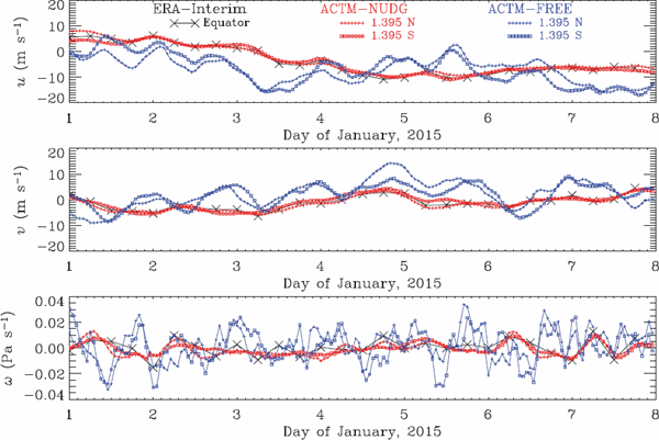
Time-series of the zonal (u), meridional (ν), and vertical (ω) wind components at grid points 0° longitude from ERA-Interim (black crosses) over the equator, together with those from ACTM nudged to ERA Interim (red) and the ACTM free run (blue) at 1.395°N and 1.395°S (the latitudes which are the closest to the equator from the available Gaussian latitudes). ERA-Interim winds are provided as instantaneous values every 6 hours, whereas ACTM winds are given as hourly averages.

6. Summary

An atmospheric general circulation model-based chemistry transport model, assimilating ERA-Interim with the nudging method, was used to assess the mean age profiles estimated from the CO₂ and SF₆ mole fractions observed during the CUBE/Biak field campaign. The age spectra corresponding to individual air samples were obtained by applying the BIER method and Lagrangian backward trajectory calculations. The BIER method has an advantage, i.e., unresolved mixing and diffusion are incorporated in the age spectra through the transport model simulation. By distinguishing specific paths of air parcels before reaching the point of interest, the Lagrangian method is capable of confirming the reliability of the transport calculations by assessing the reproducibility of the observed CO₂, SF₆, and water vapor.

The important findings are summarized as follows. The profile of CO₂ mean age is reproduced reasonably well by back trajectories, but the agreement with the BIER method is limited to below 25 km, probably due to some excessive diffusivity of the transport field in the upper tropical stratosphere. The SF₆ mean age is reproduced only below 24 km by trajectory calculations. Above 25 km, observed mole fractions (mean ages) of SF₆ are much smaller (older) than those from Lagrangian estimation. These results are consistent with the notion that the SF₆ mean age is overestimated by mixing with SF₆-depleted mesospheric air, whereas the air parcels of mesospheric origin are missing in the Lagrangian age estimation.

A valuable insight from this study concerns the use of long-duration kinematic trajectories in age estimation. Although the trajectory calculations referring to instantaneous 6-hour interval reanalysis data were unsuccessful in reproducing observed features, significant improvements were attained by using 1-hour averaged hourly wind field data provided by the AGCM assimilating the reanalysis data. This study also reconfirms the difficulty in estimating the mean age from tracer observations. The age spectra estimated from our analysis do not support the widely used assumption that the ratio of moments is constant at a value of 0.7 years. Observations of multiple trace gases and other variables independent of mean age, such as the gravitational separation (Ishidoya et al. 2013; Belikov et al. 2019, S18), will be useful to constrain the stratospheric transport features.

Supplements

This animation shows the meridional projections of Sample 8 air parcels migrating backward in time driven by three-dimensional wind of ERA-Interim, ACTM-NUDG, and ACTM-FREE meteorological fields. It runs for one year since the initialization on 27 February 2015. The black contours represent the residual stream function at ±(0.1, 0.2, 0.5, 1, 2, 4, 8, 15, 30, 50) [10² kg m⁻¹ s⁻¹]; solid and dashed contours are positive and negative values, respectively. The air parcels and the contours of zonal mean potential temperature are color-coded. The thick red lines are the zonal-mean potential vorticity [2 PVU (1 PVU = 10⁻⁶ m² s⁻¹ K kg⁻¹) in solid and 4 PVU in dashed lines] as proxies of the extratropical tropopause drawn outside of 15° latitude.

Acknowledgments

T. H. Nguyen wishes to express her gratitude to members of her laboratory, especially D. Belikov, X. Tien Nguyen-Vinh, and S. Mimura for their encouragement and discussion during her stay at the Hokkaido University. K. Ishijima and F. Hasebe are grateful to M. Takigawa and K. Miyazaki for giving a chance to attend to this work and consulting about the BIER simulation design on ACTM. Discussion with S. Ishidoya greatly inspired our study. Authors deeply thank the two anonymous reviewers as well as M. Fujiwara for their valuable and helpful comments and suggestions. This work was supported by the Japan Society for the Promotion of Science, Grant-in-Aid for Scientific Research (S) 26220101.

Appendix: List of abbreviations

References

•  Andrews,  A. E.,  K. A.  Boering,  B. C.  Daube,  S. C.  Wofsy,  M.  Loewenstein,  H.  Jost,  J. R.  Podolske,  C. R.  Webster,  R. L.  Herman,  D. C.  Scott,  G. J.  Flesch,  E. J.  Moyer,  J. W.  Elkins,  G. S.  Dutton,  D. F.  Hurst,  F. L.  Moore,  E. A.  Ray,  P. A.  Romashkin, and S.  E.  Strahan, 2001a: Mean ages of stratospheric air derived from in situ observations of CO₂, CH₄, and N₂O. J. Geophys. Res., 106, 32295-32314.
•  Andrews,  A. E.,  K. A.  Boering,  S. C.  Wofsy,  B. C.  Daube,  D. B.  Jones,  S.  Alex,  M.  Loewenstein,  J. R.  Podolske, and  S. E.  Strahan, 2001b: Empirical age spectra for the midlatitude lower stratosphere from in situ observations of CO₂: Quantitative evidence for a subtropical “barrier” to horizontal transport. J. Geophys. Res., 106, 10257-10274.
•  Arakawa,  A., and  W. H.  Schubert, 1974: Interaction of a cumulus cloud ensemble with the large-scale environment, Part I. J. Atmos. Sci., 31, 674-701.
•  Austin,  J.,  J.  Wilson,  F.  Li, and  H.  Vömel, 2007: Evolution of water vapor concentrations and stratospheric age of air in coupled chemistry-climate model simulations. J. Atmos. Sci., 64, 905-921.
•  Belikov,  D.,  S.  Sugawara,  S.  Ishidoya,  F.  Hasebe,  S.  Maksyutov,  S.  Aoki,  S.  Morimoto, and  T.  Nakazawa, 2019: Three-dimensional simulation of stratospheric gravitational separation using the NIES global atmospheric tracer transport model. Atmos. Chem. Phys., 19, 5349-5361.
•  Boering,  K. A.,  S. C.  Wofsy,  B. C.  Daube,  H. R.  Schneider,  M.  Loewenstein,  J. R.  Podolske, and  T. J.  Conway, 1996: Stratospheric mean ages and transport rates from observations of carbon dioxide and nitrous oxide. Science, 274, 1340-1343.
•  Bonazzola,  M., and  P. H.  Haynes, 2004: A trajectory-based study of the tropical tropopause region. J. Geophys. Res., 109, D20112, doi:10.1029/2003JD004356.
•  Brewer,  A. W., 1949: Evidence for a world circulation provided by the measurements of helium and water vapour distribution in the stratosphere. Quart. J. Roy. Meteor. Soc., 75, 351-363.
•  Butchart,  N., 2014: The Brewer-Dobson circulation. Rev. Geophys., 52, 157-184.
•  Chrysanthou,  A.,  A. C.  Maycock,  M. P.  Chipperfield,  S.  Dhomse,  H.  Garny,  D.  Kinnison,  H.  Akiyoshi,  M.  Deushi,  R. R.  Garcia,  P.  Jöckel,  O.  Kirner,  G.  Pitari,  D. A.  Plummer,  L.  Revell,  E.  Rozanov,  A.  Stenke,  T. Y.  Tanaka,  D.  Visioni, and  Y.  Yamashita, 2019: The effect of atmospheric nudging on the stratospheric residual circulation in chemistry-climate models. Atmos. Chem. Phys., 19, 11559-11586.
•  Colella,  P., and  P. R.  Woodward, 1984: The piecewise parabolic method (ppm) for gas-dynamic simulations. J. Comput. Phys., 54, 174-201.
•  Dee,  D. P.,  S. M.  Uppala,  A. J.  Simmons,  P.  Berrisford,  P.  Poli,  S.  Kobayashi,  U.  Andrae,  M. A.  Balmaseda,  G.  Balsamo,  P.  Bauer,  P.  Bechtold,  A. C. M.  Beljaars,  L.  van de Berg,  J.  Bidlot,  N.  Bormann,  C.  Delsol,  R.  Dragani,  M.  Fuentes,  A. J.  Geer,  L.  Haimberger,  S. B.  Healy,  H.  Hersbach,  E. V.  Hólm,  L.  Isaksen,  P.  Kållberg,  M.  Köhler,  M.  Matricardi,  A. P.  McNally,  B. M.  Monge-Sanz,  J.-J.  Morcrette,  B.-K.  Park,  C.  Peubey,  P.  de Rosnay,  C.  Tavolato,  J. N.  Thépaut, and  F.  Vitart, 2011: The ERA-Interim reanalysis: Configuration and performance of the data assimilation system. Quart. J. Roy. Meteor. Soc., 137, 553-597.
•  Diallo,  M.,  B.  Legras, and  A.  Chédin, 2012: Age of stratospheric air in the ERA-Interim. Atmos. Chem. Phys., 12, 12133-12154.
•  Dobson,  G.M. B., 1956: Origin and distribution of the polyatomic molecules in the atmosphere. Proc. Roy. Soc. London A, 236, 187-193.
•  Dragani,  R., 2011: On the quality of the ERA-Interim ozone reanalyses: Comparisons with satellite data. Quart. J. Roy. Meteor. Soc., 137, 1312-1326.
•  Elkins,  J. W.,  D. W.  Fahey,  J. M.  Gilligan,  G. S.  Dutton,  T. J.  Baring,  C. M.  Volk,  R. E.  Dunn,  R. C.  Myers,  S. A.  Montzka,  P. R.  Wamsley,  A. H.  Hayden,  J. H.  Butler,  T. M.  Thompson,  T. H.  Swanson,  E. J.  Dlugokencky,  P. C.  Novelli,  D. F.  Hurst,  J. M.  Lobert,  S. J.  Ciciora,  R. J.  McLaughlin,  T. L.  Thompson,  R. H.  Winkler,  P. J.  Fraser,  L. P.  Steele, and  M. P.  Lucarelli, 1996: Airborne gas chromatograph for in situ measurements of long-lived species in the upper troposphere and lower stratosphere. Geophys. Res. Lett., 23, 347-350.
•  Engel,  A.,  T.  Möbius,  H.  Bönisch,  U.  Schmidt,  R.  Heinz,  I.  Levin,  E.  Atlas,  S.  Aoki,  T.  Nakazawa,  S.  Sugawara,  F.  Moore,  D.  Hurst,  J.  Elkins,  S.  Schauffler,  A.  Andrews, and  K.  Boering, 2009: Age of stratospheric air unchanged within uncertainties over the past 30 years. Nat. Geosci., 2, 28-31.
•  Engel,  A.,  M.  Strunk,  M.  Müller,  H.-P.  Haase,  C.  Poss,  I.  Levin, and  U.  Schmidt, 2002: Temporal development of total chlorine in the high-latitude stratosphere based on reference distributions of mean age derived from CO₂ and SF₆. J. Geophys. Res., 107, D12, 4136, doi:10.1029/2001JD000584.
•  Engel,  A.,  H.  Bönisch,  M.  Ullrich,  R.  Sitals,  O.  Membrive,  F.  Danis, and  C.  Crevoisier, 2017: Mean age of stratospheric air derived from Air-Core observations. Atmos. Chem. Phys., 17, 6825-6838.
•  Fritsch,  F.,  H.  Garny,  A.  Engel,  H.  Bönisch, and  R.  Eichinger, 2020: Sensitivity of age of air trends to the derivation method for non-linear increasing inert SF₆. Atmos. Chem. Phys., 20, 8709-8725.
•  Fueglistaler,  S.,  M.  Bonazzola,  P. H.  Haynes, and  T.  Peter, 2005: Stratospheric water vapor predicted from the Lagrangian temperature history of air entering the stratosphere in the tropics. J. Geophys. Res., 110, D08107, doi:10.1029/2004JD005516.
•  Garcia,  R. R.,  W. J.  Randel, and  D. E.  Kinnison, 2011: On the determination of age of air trends from atmospheric trace species. J. Atmos. Sci., 68, 139-154.
•  Haine,  T. W. N.,  H.  Zhang,  D. W.  Waugh, and  M.  Holzer, 2008: On transit-time distributions in unsteady circulation models. Ocean Modell., 21, 35-45.
•  Hall,  T. M., and  R. A.  Plumb, 1994: Age as a diagnostic of stratospheric transport. J. Geophys. Res., 99, 1059-1070.
•  Hall,  T. M.,  D. W.  Waugh,  K. A.  Boering, and  R. A.  Plumb, 1999: Evaluation of transport in stratospheric models. J. Geophys. Res., 104, 18815-18839.
•  Harnisch,  J.,  R.  Borchers,  P.  Fabian, and  M.  Maiss, 1996: Tropospheric trends for CF₄ and C₂F₆ since 1982 derived from SF₆ dated stratospheric air. Geophys. Res. Lett., 23, 1099-1102.
•  Hasebe,  F., and  T.  Noguchi, 2016: A Lagrangian description on the troposphere-to-stratosphere transport changes associated with the stratospheric water drop around the year 2000. Atmos. Chem. Phys., 16, 4235-4249.
•  Hasebe,  F.,  S.  Aoki,  S.  Morimoto,  Y.  Inai,  T.  Nakazawa,  S.  Sugawara,  C.  Ikeda,  H.  Honda,  H.  Yamazaki,  Halimurrahman,  N.  Komala,  F.  Putri,  A.  Budiyono,  M.  Soedjarwo,  S.  Ishidoya,  S.  Toyoda,  T.  Shibata,  M.  Hayashi,  N.  Eguchi,  N.  Nishi,  M.  Fujiwara,  S.  Ogino,  M.  Shiotani, and  T.  Sugidachi, 2018: Coordinated Upper-Troposphere-to-Stratosphere Balloon Experiment in Biak. Bull. Amer. Meteor. Soc., 99, 1213-1230.
•  Hauck,  M.,  F.  Fritsch,  H.  Garny, and  A.  Engel, 2019: Deriving stratospheric age of air spectra using an idealized set of chemically active trace gases. Atmos. Chem. Phys., 19, 5269-5291.
•  Hauck,  M.,  H.  Bönisch,  P.  Hoor,  T.  Keber,  F.  Ploeger,  T. J.  Schuck, and  A.  Engel, 2020: A convolution of observational and model data to estimate age of air spectra in the northern hemispheric lower stratosphere. Atmos. Chem. Phys., 20, 8763-8785.
•  Ishidoya,  S.,  S.  Sugawara,  S.  Morimoto,  S.  Aoki,  T.  Nakazawa,  H.  Honda, and  S.  Murayama, 2013: Gravitational separation in the stratosphere - A new indicator of atmospheric circulation. Atmos. Chem. Phys., 13, 8787-8796.
•  Ishijima,  K.,  P. K.  Patra,  M.  Takigawa,  T.  Machida,  H.  Matsueda,  Y.  Sawa,  L. P.  Steele,  P. B.  Krummel,  R. L.  Langenfelds,  S.  Aoki, and  T.  Nakazawa, 2010: Stratospheric influence on the seasonal cycle of nitrous oxide in the troposphere as deduced from aircraft observations and model simulations. J. Geophys. Res., 115, D20308, doi:10.1029/2009JD013322.
•  Ishijima,  K.,  M.  Takigawa,  K.  Sudo,  S.  Toyoda,  N.  Yoshida,  T.  Röckmann,  J.  Kaiser,  S.  Aoki,  S.  Morimoto,  S.  Sugawara, and  T.  Nakazawa, 2015: Development of an atmospheric N₂O isotopocule model and optimization procedure, and application to source estimation. Atmos. Chem. Phys. Discuss., 15, 19947-20011.
•  Kida,  H., 1983: General circulation of air parcels and transport characteristics derived from a hemispheric GCM. Part 2. Very long-term motions of air parcels in the troposphere and stratosphere. J. Meteor. Soc. Japan, 61, 510-523.
•  Kinoshita,  T.,  K.  Sato,  K.  Ishijima,  M.  Takigawa, and  Y.  Yamashita, 2019: Formulation of three-dimensional quasi-residual mean flow balanced with diabatic heating rate and potential vorticity flux. J. Atmos. Sci., 76, 851-863.
•  Krol,  M.,  M.  de Bruine,  L.  Killaars,  H.  Ouwersloot,  A.  Pozzer,  Y.  Yin,  F.  Chevallier,  P.  Bousquet,  P.  Patra,  D.  Belikov,  S.  Maksyutov,  S.  Dhomse,  W.  Feng, and  M. P.  Chipperfield, 2018: Age of air as a diagnostic for transport timescales in global models. Geosci. Model Dev., 11, 3109-3130.
•  Li,  D., and  K. P.  Shine, 1999: UK Universities Global Atmospheric Modelling Programme (UGAMP) Global Ozone Climatology Project dataset. NCAS British Atmospheric Data Centre. [Available at https://catalogue.ceda.ac.uk/uuid/bff84b935ce5aa9f04624777b0eea507.]
•  Li,  F.,  D. W.  Waugh,  A. R.  Douglass,  P. A.  Newman,  S.  Pawson,  R. S.  Stolarski,  S. E.  Strahan, and  J. E.  Nielsen, 2012a: Seasonal variations of stratospheric age spectra in the Goddard Earth Observing System Chemistry Climate Model (GEOSCCM). J. Geophys. Res., 117, D05134, doi:10.1029/2011JD016877.
•  Li,  F.,  D. W.  Waugh,  A. R.  Douglass,  P. A.  Newman,  S. E.  Strahan,  J.  Ma,  J. E.  Nielsen, and  Q.  Liang, 2012b: Long-term changes in stratospheric age spectra in the 21st century in the Goddard Earth Observing System Chemistry-Climate Model (GEOSCCM). J. Geophys. Res., 117, D20119, doi:10.1029/2012JD017905.
•  Lin,  S.-J., and  R. B.  Rood, 1996: Multidimensional fluxform semi-Lagrangian transport schemes. Mon. Wea. Rev., 124, 2046-2070.
•  Machida,  T.,  H.  Matsueda,  Y.  Sawa,  Y.  Nakagawa,  K.  Hirotani,  N.  Kondo,  K.  Goto,  T.  Nakazawa,  K.  Ishikawa, and  T.  Ogawa, 2008: Worldwide measurements of atmospheric CO₂ and other trace gas species using commercial airlines. J. Atmos. Oceanic Technol., 25, 1744-1754.
•  Matsueda,  H.,  T.  Machida,  Y.  Sawa, and  Y.  Niwa, 2015: Long-term change of CO₂ latitudinal distribution in the upper troposphere. Geophys. Res. Lett., 42, 2508-2514.
•  McFarlane,  N. A., 1987: The effect of orographically excited gravity wave drag on the general circulation of the lower stratosphere and troposphere. J. Atmos. Sci., 44, 1775-1800.
•  Mellor,  G. L., and  T.  Yamada, 1982: Development of a turbulence closure model for geophysical fluid problems. Rev. Geophys., 20, 851-875.
•  Mote,  P. W.,  K. H.  Rosenlof,  M. E.  McIntyre,  E. S.  Carr,  J. C.  Gille,  J. R.  Holton,  J. S.  Kinnersley,  H. C.  Pumphrey,  J. M.  Russell III, and  J. W.  Waters, 1996: An atmospheric tape recorder: The imprint of tropical tropopause temperatures on stratospheric water vapor. J. Geophys. Res., 101, 3989-4006.
•  Nakazawa,  T.,  T.  Machida,  S.  Sugawara,  S.  Murayama,  S.  Morimoto,  G.  Hashida,  H.  Honda, and  T.  Itoh, 1995: Measurements of the stratospheric carbon dioxide concentration over Japan using a balloon-borne cryogenic sampler. Geophys. Res. Lett., 22, 1229-1232.
•  Neu,  J. L., and  R. A.  Plumb, 1999: Age of air in a “leaky pipe” model of stratospheric transport. J. Geophys. Res., 104, 19243-19255.
•  Numaguti,  A.,  M.  Takahashi,  T.  Nakajima, and  A.  Sumi, 1997: Description of CCSR/NIES Atmospheric General Circulation Model. CGER's Supercomput. Monogr. Rep. 3, Natl. Inst. for Environ. Stud., Tsukuba, Japan, 48 pp.
•  Onogi,  K.,  J.  Tsutsui,  H.  Koide,  M.  Sakamoto,  S.  Kobayashi,  H.  Hatsushika,  T.  Matsumoto,  N.  Yamazaki,  H.  Kamahori,  K.  Takahashi,  S.  Kadokura,  K.  Wada,  K.  Kato,  R.  Oyama,  T.  Ose,  N.  Mannoji, and  R.  Taira, 2007: The JRA-25 reanalysis. J. Meteor. Soc. Japan, 85, 369-432.
•  Patra,  P. K.,  S.  Lal,  B. H.  Subbaraya,  C. H.  Jackman, and  P.  Rajaratnam, 1997: Observed vertical profile of sulphur hexafluoride (SF₆) and its atmospheric applications. J. Geophys. Res., 102, 8855-8859.
•  Patra,  P.,  M.  Takigawa,  G. S.  Dutton,  K.  Uhse,  K.  Ishijima,  B. R.  Lintner,  K.  Miyazaki, and  J. W.  Elkins, 2009: Transport mechanisms for synoptic, seasonal and interannual SF₆ variations and “age” of air in troposphere. Atmos. Chem. Phys., 9, 1209-1225.
•  Patra,  P. K.,  M.  Takigawa,  S.  Watanabe,  N.  Chandra,  K.  Ishijima, and  Y.  Yamashita, 2018: Improved chemical tracer simulation by MIROC4.0-based atmospheric chemistry-transport model (MIROC4-ACTM). SOLA, 14, 91-96.
•  Ploeger,  F., and  T.  Birner, 2016: Seasonal and inter-annual variability of lower stratospheric age of air spectra. Atmos. Chem. Phys., 16, 10195-10213.
•  Plumb,  R. A., 1996: A “tropical pipe” model of stratospheric transport. J. Geophys. Res., 101, 3957-3972.
•  Plumb,  R. A., and  J.  Eluszkiewicz, 1999: The Brewer- Dobson circulation: Dynamics of the tropical upwelling. J. Atmos. Sci., 56, 868-890.
•  Podglajen,  A., and  F.  Ploeger, 2019: Retrieving the age of air spectrum from tracers: Principle and method. Atmos. Chem. Phys., 19, 1767-1783.
•  Ray,  E. A.,  F. L.  Moore,  J. W.  Elkins,  K. H.  Rosenlof,  J. C.  Laube,  T.  Röckmann,  D. R.  Marsh, and  A. E.  Andrews, 2017: Quantification of the SF₆ lifetime based on mesospheric loss measured in the stratospheric polar vortex. J. Geophys. Res.: Atmos., 122, 4626-4638.
•  Reddmann,  T.,  R.  Ruhnke, and  W.  Kouker, 2001: Three-dimensional model simulations of SF₆ with mesospheric chemistry. J. Geophys. Res., 106, 14525-14537.
•  Reithmeier,  C.,  R.  Sausen, and  V.  Grewe, 2008: Investigating lower stratospheric model transport: Lagrangian calculations of mean age and age spectra in the GCM ECHAM4. Climate Dyn., 30, 225-238.
•  Sawa,  Y.,  T.  Machida, and  H.  Matsueda, 2008: Seasonal variations of CO₂ near the tropopause observed by commercial aircraft. J. Geophys. Res., 113, D23301, doi:10.1029/2008JD010568.
•  Schmidt,  U.,  G.  Kulessa,  E.  Klein,  E.-P.  Röth,  P.  Fabian, and  R.  Borchers, 1987: Intercomparison of balloon-borne cryogenic whole air samplers during the MAP/GLOBUS 1983 campaign. Planet. Space Sci., 35, 647-656.
•  Schoeberl,  M. R.,  A. R.  Douglass,  Z.  Zhu, and  S.  Pawson, 2003: A comparison of the lower stratospheric age spectra derived from a general circulation model and two data assimilation systems. J. Geophys. Res., 108, 4113, doi:10.1029/2002JD002652.
•  Schoeberl,  M. R.,  A. R.  Douglass,  B.  Polansky,  C.  Boone,  K. A.  Walker, and  P.  Bernath, 2005: Estimation of stratospheric age spectrum from chemical tracers. J. Geophys. Res., 110, D21303, doi:10.1029/2005JD006125.
•  Stiller,  G. P.,  T.  von Clarmann,  F.  Haenel,  B.  Funke,  N.  Glatthor,  U.  Grabowski,  S.  Kellmann,  M.  Kiefer,  A.  Linden,  S.  Lossow, and  M.  López-Puertas, 2012: Observed temporal evolution of global mean age of stratospheric air for the 2002 to 2010 period. Atmos. Chem. Phys., 12, 3311-3331.
•  Sugawara,  S.,  S.  Ishidoya,  S.  Aoki,  S.  Morimoto,  T.  Nakazawa,  S.  Toyoda,  Y.  Inai,  F.  Hasebe,  C.  Ikeda,  H.  Honda,  D.  Goto, and  F. A.  Putri, 2018: Age and gravitational separation of the stratospheric air over Indonesia. Atmos. Chem. Phys., 18, 1819-1833.
•  Waugh,  D., and  T.  Hall, 2002: Age of stratospheric air: Theory, observations, and models. Rev. Geophys., 40, 1010, doi:10.1029/2000RG000101.