Abstract
We analyze a multi-model ensemble at a convection-resolving resolution based on the DYAMOND models and a resolution ensemble based on the limited-area model COSMO over 40 days to study how tropical and subtropical marine low clouds are represented at a kilometer-scale resolution.
The analyzed simulations produce low cloud fields that look in general realistic in comparison with satellite images. The evaluation of the radiative balance, however, reveals substantial inter-model differences and an underestimated low cloud cover in most models. Models that simulate increased low cloud cover are found to have a deeper marine boundary layer (MBL), stronger entrainment, and an enhanced latent heat flux. These findings demonstrate that some of the fundamental relations of the MBL are systematically represented by the model ensemble, which implies that the relevant dynamical processes start to become resolved on the model grid at a kilometer-scale resolution. A sensitivity experiment with the COSMO model suggests that differences in the strength of turbulent vertical mixing may contribute to the inter-model spread in cloud cover.
1. Introduction
A fundamental problem in climate projection is our inability to evaluate in time whether or not the model predictions are correct, i.e., before the projected changes will have occurred. This makes uncertainty estimation, for instance, by the use of ensemble simulations or by model inter-comparison, an important pillar of climate change research. The equilibrium climate sensitivity (ECS) (Stevens et al. 2016; Sherwood et al. 2020) is probably the most fundamental measure for the impact of human greenhouse gas emissions on the climate system – and its inter-model spread has long been a source of concern. Although global climate models have evolved substantially over the last decades, the spread in the estimates of ECS produced by the models has not been reduced; if anything, it has increased (Charney et al. 1979; Collins et al. 2013; Sherwood et al. 2020; Zelinka et al. 2020). Fortunately, the understanding of the underlying problem did improve (Boucher et al. 2013; Bony et al. 2015; Schneider et al. 2017). The main source of uncertainty in ECS is cloud radiative feedbacks (Soden and Held 2006), primarily caused by changes in low cloud cover with a warming climate (Zelinka et al. 2016). Especially tropical and subtropical low clouds show disagreement between climate models and observations, and their response to a warming climate differs substantially among models (Bony and Dufresne 2005). Tropical and subtropical low clouds (which for brevity we refer to as “low clouds”) thus lie at the heart of the uncertainty in our climate projections and motivate our study of the ability of a new class of models to represent them.
The two most prevalent low cloud types are stratocumulus clouds and trade wind cumuli (Warren et al. 1986, 1988). Stratocumulus clouds are particularly abundant over the eastern parts of the subtropical ocean basins owing to the large-scale subsidence, the strong lower-tropospheric stability, and the available moisture supply at the surface, typical for these regions (Wood 2012). Stratocumulus clouds consist of a shallow stratiform cloud layer at the top of the marine boundary layer (MBL) that is capped by a strong temperature inversion (e.g., Neiburger et al. 1961). In addition, the stratocumulus-topped MBL is strewn with convective cells, the downdrafts of which are driven by negative buoyancy due to longwave radiative cooling of the stratiform cloud layer (Lilly 1968). While the convective circulations can couple the stratiform cloud layer to the moisture source at the ocean surface (e.g., Nicholls 1984), they also entrain relatively warm and dry free-tropospheric air across the inversion, drying the MBL and causing a vertical growth of the MBL over time (Bretherton and Wyant 1997; Stevens 2007; Mellado 2017). The drying and deepening of the MBL reduce the near-surface relative humidity and increase the surface latent heat flux, thereby modulating the sea-surface temperature (Hourdin et al. 2015). The entrainment rate at the inversion is stronger if the inversion is weak (Deardorff 1980). Even though entrainment dilutes the clouds, it often helps deepen the cloud layer by lifting the cloud top more than the cloud base (Randall 1984). As the MBL experiences higher sea-surface temperature towards the equator and the convective buoyancy production at the surface is enhanced, the entrainment drying becomes stronger and cannot be sufficiently balanced by radiative cooling. Eventually, the stratiform cloud layer evaporates, which marks the transition from the stratocumulus-topped MBL to the trade-wind cumulus regime (Wyant et al. 1997).
The main reason for the large inter-model spread in low clouds lies in the fact that the formation and dissipation of these clouds are controlled by dynamical motions occurring at small scales on the order of 0.1–10 km, whereas the horizontal grid spacing of climate models typically ranges between 50 km and 100 km. This scale gap has to be bridged by convective parameterizations, which partly rely on empirical relations and do not necessarily describe in a physically consistent manner the interplay between clouds and their environment, for instance, through convective and turbulent mixing and radiative cooling (e.g., Brient et al. 2016; Vial et al. 2016). As a result, clouds need not be located in the right place (e.g., Teixeira et al. 2011), and their vertical structure is unresolved. Consequently, the specific representation of shallow convection in a model can have a fundamental effect on the simulated climate sensitivity (Zhang et al. 2013; Sherwood et al. 2014; Qu et al. 2014).
Using higher model resolution, this gap between the grid scale and the dynamical scales of low clouds can be partially closed (0.1–1 km; sub-kilometerscale models) or reduced (1–10 km; kilometer-scale models). Specifically, large-eddy simulations (LESs) with a resolution between 0.05 km and 0.5 km (e.g., Stevens et al. 2005; Ackerman et al. 2009; Zhang et al. 2013; Nuijens and Siebesma 2019) resolve much of the interaction between low clouds and their environment. Such interactions include, for instance, mixing and evaporation at cloud boundaries and the formation of downdrafts (e.g., de Roode and Bretherton 2003; Noda et al. 2013) as well as cold-pool dynamics, which affect cloud aggregation (e.g., Seifert and Heus 2013). The benefits of representing such interactions are confirmed by converging cloud size distributions in LESs (Heus and Seifert 2013). However, a major problem of LESs in the context of climate projection is that the domain size is typically restricted to a few hundred kilometers. This necessitates the parameterization of the meso- and large-scale atmospheric circulation introducing new uncertainties.
Larger domains can be simulated using kilometer-scale models which have become very popular over the last decade, mainly in the context of the deep convection parameterization that can be avoided within or approaching the kilometer scale (Prein et al. 2015; Leutwyler et al. 2016; Vergara-Temprado et al. 2020). The most prominent class of kilometer-scale models is the convection-resolving model (CRM), with a horizontal grid spacing of below approximately 5 km (Prein et al. 2015). While these models were originally run on limited-area domains (e.g., Ban et al. 2014; Leutwyler et al. 2016; Ito et al. 2017; Stevens et al. 2020), running global or near-global CRMs during short periods have recently gained a lot of attention (Miyamoto et al. 2013; Bretherton and Khairoutdinov 2015; Fuhrer et al. 2018; Satoh et al. 2019). The model inter-comparison project “The DYnamics of the Atmospheric general circulation Modeled On Non-hydrostatic Domains (DYAMOND)” (Stevens et al. 2019) is a pioneering effort in this direction. Nine global atmospheric models were run at a convection-resolving resolution to simulate a 40-day period. The atmospheric circulation is fully resolved in these simulations from the synoptic down to the convective scale, allowing for an unprecedented comprehension of the climate system in all its complexities (e.g., Dueben et al. 2020; Arnold et al. 2020).
Although CRMs cannot describe small-scale atmospheric motions with the same degree of detail as LESs, they may provide a good compromise between accuracy vs. domain size and integration period. The finer model grid of CRMs compared with conventional climate models resolves a larger fraction of the convective motions within the MBL, which can reduce low cloud biases (Hohenegger et al. 2020). In this respect, the most fundamental difference from coarser simulations is the ability to partially resolve nonhydrostatic vertical motions on the model grid (Stevens et al. 2020), which is a milestone on the path to a physically consistent coupling between clouds and their environment. At the same time, we should not expect CRMs to solve the “low cloud problem”, given that most features of the MBL are still under-resolved. For instance, the differentiation between cumulus and stratiform clouds has been found to be considerably less successful at a kilometer-scale resolution compared with the LES resolution (Stevens et al. 2020). Given that kilometer-scale climate simulations are expected to become feasible in the near future (Schär et al. 2020), gaining more experience in how these models simulate low clouds is desirable. In this study, we will systematically analyze the cloud field and the structure of the MBL in the set of global DYAMOND CRMs, with the aim of quantifying and better understanding the drivers of inter-model variability in the simulation of low clouds at a convection-resolving resolution. We will further assess the sensitivities to model resolution in a specific CRM, the limited-area model COSMO. In the following section, the experimental setup and the analysis methods are presented. The results are shown in Section 3 and discussed and concluded in Sections 4 and 5.
2. Methods
2.1 Experimental Setup
In this study, we analyze a set of kilometer-scale simulations that were run by 10 different models to study the representation of low clouds. The main analysis region is located over the South-East Atlantic, as indicated by the red dashed rectangle in Fig. 1. This subtropical-to-tropical domain is predominantly covered by stratocumulus clouds, but it also encompasses the transition to trade-wind cumuli. The analysis domain thus contains the two dominant low cloud types with a focus on stratocumulus clouds. The South-East Atlantic low cloud region is comparable with the one in the South-East Pacific in terms of the large-scale forcing, like the sea-surface temperature, subsidence, and trade-wind strength (Noda and Satoh 2014). The exact location of the analysis domain is chosen based on the largest observed low cloud cover during the period considered. The simulations cover a 40-day-long period between 1st August and 9 September 2016. If not indicated otherwise, the first 5 days are considered as a spin-up and excluded from the analysis, resulting in a total of 35 days to compute statistics.

Out of the 18 analyzed simulations, 13 simulations (from 9 different models) are provided by the DYAMOND project, whereas the other 5 simulations are conducted with the limited-area model COSMO, as described below. The set of simulations is listed in Table 1 with the name of the model used, approximate horizontal grid spacing (Δx), and whether or not a shallow convection scheme is employed. The high-resolution DYAMOND members are run at a grid spacing between 2 km < Δx ≤ 5 km. These 9 simulations in combination with the COSMO 2.2 simulation are considered to be the core of this study and analyzed in detail in the sense of a model intercomparison. The remaining DYAMOND members with a grid spacing Δx > 5 km extend the analysis whenever useful. The 5 COSMO simulations covering resolutions from 12 km to 0.5 km are used to assess the role of horizontal resolution. Two additional sensitivity simulations on the role of turbulence are discussed in Section 3.3e.

The COSMO model is driven at its lateral boundaries by the European Centre for Medium-Range Weather Forecast (ECMWF) Re-analysis (ERA5) [Copernicus Climate Change Service (C3S) 2017] (see below). The prescribed lateral forcing will draw the limited-area COSMO runs closer to observations for variables that are controlled by the large-scale flow. The goal of this study is, however, not to compare the performance between limited-area and global models but rather to assess inter-model variability (DYAMOND simulations) and sensitivity to horizontal resolution (COSMO simulations).
a. DYAMOND simulations
The DYAMOND model intercomparison project (Stevens et al. 2019) involves the following models (only acronyms given): NICAM, SAM, ICON, UM, MPAS, IFS, GEOS, ARPEGE-NH, and FV3. The technical description of these models can be found on the ESiWACE web page1 where the project is hosted. The experimental setup is described in the study by Stevens et al. (2019) and only briefly summarized here. The global models are initialized with the global (9-km) operational meteorological analysis from the ECMWF. The operational daily sea-surface temperature from the ECMWF is used as the initial and lower boundary condition over the ocean. Soil initialization over land is subject to the practices of the individual modeling groups. In general, the experimental protocol was kept as simple as possible to encourage participation (Stevens et al. 2019).
b. COSMO simulations
Since the COSMO simulations were performed for the purposes of this study, the model is described here in more detail. The COSMO model solves the fully compressible atmospheric equations. It has originally been developed as a numerical weather prediction model (Steppeler et al. 2003) and later evolved into a regional climate model (Jaeger et al. 2008; Rockel et al. 2008). The version used in this study employs a dynamical core adapted for hybrid GPU-CPU architectures (Fuhrer et al. 2014; Leutwyler et al. 2016) for the sake of higher computational performance. The model represents the horizontal and vertical dimensions on a rotated latitude-longitude grid and a generalized Gal-Chen coordinate, respectively. The time integration is performed with a split-explicit third-order Runge-Kutta scheme (Klemp and Wilhelmson 1978; Wicker and Skamarock 2002). Temperature, pressure, as well as horizontal and vertical winds are discretized with a fifth-order advection scheme, whereas moist quantities are integrated using a positive-definite second-order scheme (Bott 1989). Deep and shallow convection parameterizations are switched off in all simulations as in a previous study using the COSMO model, this was found to reduce the bias in the shortwave radiative balance at a kilometer-scale resolution (Vergara-Temprado et al. 2020). Radiative fluxes are computed following the δ -two-stream approach described by Ritter and Geleyn (1992). The single-moment bulk scheme described by Reinhardt and Seifert (2006) is used to parameterize cloud microphysics. For the computation of subgrid-scale vertical turbulent fluxes, a 1D TKE-based model (Raschendorfer 2001) is employed. The minimum threshold for eddy diffusivity for heat and momentum under stable conditions is set to 0.4 m2 s−1 (Possner et al. 2014). The vertical turbulent length scale is set to 100 m in all simulations (consistent with the employment of identical vertical levels in all simulations) with the exception of a few sensitivity tests (see Section 3.3e.). In the horizontal directions, turbulent diffusion is used and computed using a Smagorinsky-Lilly closure (Baldauf and Zängl 2012). Over land, the second-generation land-surface model TERRA_ML (Heise et al. 2003) with the groundwater-runoff scheme described by Schlemmer et al. (2018) is used. Over the ocean, the COSMO model uses the prescribed sea-surface temperature.
The setup of the COSMO simulations is outlined in Fig. 1. COSMO 12 (494 × 439 × 60 grid points) and COSMO 4.4 (1350 × 1200 × 60 grid points) are initialized and laterally driven with the ERA5 reanalysis data at 1-hourly increments. COSMO 2.2 (2100 × 1180 × 60 grid points), COSMO 1.1 (3200 × 1830 × 60 grid points), and COSMO 0.5 (5300 × 3100 × 60 grid points) are one-way nested into and initialized from the COSMO 4.4 run. All simulations are identically run with 60 vertical levels that range between the surface and an altitude of approximately 30 km. The vertical grid spacing is 20 m at the surface and approximately 180 m at a 1-km altitude. At the lower boundary, the operational daily sea-surface temperature from the ECMWF is used over ocean grid points, and the soil moisture profile on land grid points is initialized based on a 17-year-long COSMO simulation run at 24 km Δx. The only methodological difference in the initialization between the COSMO and the DYAMOND simulations is thus that the atmospheric state in COSMO is initialized using ERA5 instead of the ECMWF operational analysis. The effect of this was found to be negligible. The ITCZ is included within the COSMO 4.4 domain to have a model-internal representation of the Hadley cell as an important large-scale driver of low clouds. This should make the COSMO members better comparable with the DYAMOND members by allowing for more comparable variability in the dynamics of the limitedarea simulations.
2.3 Observations and reanalysis data sets
The following data sets are used for the evaluation of the model simulations:
-
• The Satellite Application Facility on Climate Monitoring (CM SAF) top of the atmosphere radiation (Urbain et al. 2017), based on the Meteosat Visible Infra-Red Imager (MVIRI) and the Spinning Enhanced Visible and Infrared Imager (SEVIRI), is used to evaluate the simulated radiative balance at the top of the atmosphere. It has a spatial resolution of approximately 45 km and provides daily mean radiative fluxes.
-
• The CM SAF cloud fractional cover (Stöckli et al. 2017) provides hourly values of the observed instantaneous low cloud fraction at a spatial resolution of approximately 5 km.
-
• The CM SAF Advanced Television Infrared Observation Satellite Operational Vertical Sounder (ATOVS) (Courcoux and Schröder 2015) provides daily mean values of the observed tropospheric water vapor between the surface and 200 hPa at a 90-km spatial resolution.
-
• The Visible Infrared Imaging Radiometer Suite (VIIRS) (Cao 2014) is aboard the JPSS-1 satellite and provides visible images based on the I1, M4, and M3 spectral bands at a 250-m spatial resolution around noon with a daily frequency.
-
• The ERA5 [Copernicus Climate Change Service (C3S) 2017] is a gridded reanalysis data set at a spatial resolution of 31 km. It is used at a 3-hourly temporal frequency to provide a partly observationalbased reference when analyzing variables for which satellite observations are unavailable.
To analyze the simulated low cloud amount, both the amount of cloud water and the cloud fraction are used. However, the diagnosed low cloud fraction is available in the output of only 3 models (COSMO, IFS, and ARPEGE-NH). As a workaround, the liquid water path (LWP - vertically integrated cloud liquid water) is used to approximate the low cloud fraction described by, e.g., Vergara-Temprado et al. (2018). If the LWP exceeds 1 g m−2, the grid column is considered to be covered by low clouds. The chosen threshold is low, but the dependence of the resulting cloud fraction on the exact value has been tested and found to be weak. The outlined procedure is based on two key assumptions: First, due to the large-scale subsidence, mid-level clouds are rare (Warren et al. 1988). If they exist, they should be rooted in low clouds that grow to higher levels. The latter implies that the midcloud fraction should be a subset of the low cloud fraction. Second, high clouds are composed of ice and not part of the LWP. These assumptions were tested using ERA5 and were found to be fulfilled reasonably well.
b. Inversion
The vertical extent (or depth) of the MBL is defined as the distance between the surface and the inversion. The latter is defined at the height where the vertical gradient in the virtual temperature is the largest and positive. Over the domain considered, an inversion according to this definition exists in all models in at least 98.8 % of the grid columns. Columns at time steps without inversion are excluded from the analyses that depend on the inversion. The inversion strength is computed as the difference in the virtual potential temperature between the levels of maximum absolute virtual temperature above and minimum absolute virtual temperature below the inversion.
c. Relative vertical profiles
Because the height of the inversion varies in space and time, direct horizontal and temporal averaging leads to mean vertical profiles where the sharp gradients in atmospheric quantities at the inversion are smeared out. Models with stronger variability in the inversion height thus appear to have smoother gradients across the inversion. Vertical profiles will therefore also be presented relative to the local MBL depth, as described by, e.g., Lilly (2002). The procedure is as follows: For each model column, the vertical coordinate (already transformed to height) is expressed relative to the inversion height such that, for instance, a value of 1.0 represents the local inversion height (used to represent the top of the MBL), and a value of 0.5 represents half the local inversion height. Subsequently, the model variables are interpolated to identical relative height in each model column and then averaged over the analysis domain in this framework.
d. Diabatic heating
The diabatic heating term is not part of the model output but is diagnosed from the available fields. The diabatic heating θ̇ is defined as
Under quasi-steady conditions, it can be diagnosed from
To do so, we use the three-dimensional model output and express the ∇
θ-term using centred finite differences. This yields an estimate of
θ̇ (
x, y, z, t) for the whole computational volume at each available output time. Over the analyzed time window of 35 days, the assumption of a steady state is justified when comparing the long-term temperature tendency (less than 5 K in 35 days) with the local tendency due to subsidence at the inversion (≈ 6 K per day). The temporal average is denoted as

, and it is computed from the diagnosed instantaneous values using 3-hourly model output. For display, we will present the mean vertical profiles averaged over the entire analysis domain.
In addition, we distinguish between the mean-flow and eddy contributions. To this end, all variables are expressed as
where

denotes the 35-day average, and
θ̇′ denotes the time-dependent deviation thereof. With this notation and using Reynolds decomposition and averaging, (2) can be expressed as
The mean term
v̄ · ∇
θ̄ is directly determined from the time-mean fields, whereas the eddy term

is obtained as a residual from (4) using
θ̇ as computed in (2).
The diabatic heating diagnosed from (4) is the sum of the heating due to sub-grid-scale fluxes H (turbulence and the convection schemes), and due to microphysics M and radiation R:
The individual contributions of
H, M, and
R cannot be diagnosed based on the available output.
c. Entrainment
To define the entrainment velocity E at the inversion, we start from the prognostic equation for the MBL height (e.g., Stevens 2006):
where
zi denotes is the local inversion height;
vi, the horizontal wind vector at the inversion; and
wi, the vertical motion at the inversion.
Equation (6) is here evaluated as a spatial and temporal average of the three-dimensional instantaneous velocity field. Under quasi-steady conditions, (6) can be simplified to
Equation (7) is used to interpret the lateral growth of the MBL due to entrainment.
3. Results
3.1 Cloud structures
Figures 2a–j present a snapshot of the cloud field after 2 weeks of simulation time on 14 August 2016 at 12:00 UTC as simulated by the members of the CRM intercomparison. The cloud field is represented by the LWP. Figure 2k presents a satellite picture (VIIRS, corrected reflectance) taken around noon on the same day. The satellite picture gives an impression of how the cloud field looks in reality and serves for a qualitative comparison only. In particular, after 2 weeks of simulation time, the DYAMOND models manifest weather that may differ substantially from the instantaneous weather of the satellite observation due to predictability limitations.

From a visual perspective, the models produce different-looking cloud structures, but in some models, they resemble the ones in the satellite estimate. The cellular nature of stratocumulus clouds is well visible in some simulations (e.g., FV3 3.25 and GEOS 3), whereas in others, the stratiform character of the cloud field appears to be more pronounced (e.g., UM 5, IFS 4, and ARPEGE-NH 2.5).
Figures 2l–p present a close-up view of the cloud field simulated by the COSMO simulations at increasing horizontal resolution on the smaller snapshot domain (see Fig. 1). Besides the expected increase in detail with higher model resolution, the cloud fraction strongly decreases from COSMO 12 to COSMO 2.2 but then becomes less sensitive at even higher resolution.
3.2 Radiative fluxes
a. Shortwave radiative flux
Measurements of the shortwave radiative flux at the top of the atmosphere provide a more objective evaluation of the simulated low cloud cover. Since the effect of thin high clouds on shortwave radiation is small, the albedo at the top of the atmosphere can be taken as a proxy for the amount of low clouds over the region considered. Figures 3a–j present the model intercomparison of the spatial distribution of the 35-day mean albedo (from 6 August 2016, 00:00 UTC, to 9 September, 24:00 UTC). Figures 3k and 3l present the albedo in the ERA5 and the CM SAF data record. Most simulations produce a region of enhanced albedo similar to the observation, although its magnitude is underestimated in most of them. The underestimation ranges from values indicating only intermittent cloud cover (MPAS 3.75 and NICAM 3.5) up to close agreement with the observed albedo (UM 5, FV3 3.25, ICON 2.5, COSMO 2.2). These differences are already present at the start of the simulation and remain relatively constant throughout the simulation period (not shown).

A limitation of using the top of the atmosphere albedo as a proxy for the low cloud cover is that intermodel differences could stem from differences either in the cloud fraction or in the cloud albedo. The albedo of low clouds is affected by their LWP, by microphysical cloud properties, and by how the radiation scheme translates cloud properties into scattering of shortwave radiation. Although the eventual goal is that the models correctly simulate the radiative fluxes at the top of the atmosphere, we will in the following assess the sensitivity of the simulated albedo to these cloud characteristics.
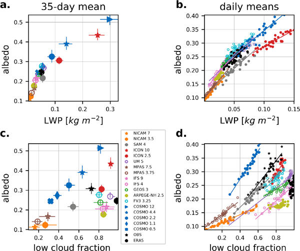
Figure 4 presents the relation between domain averages of the albedo and the LWP (Figs. 4a, b), and between the albedo and the low cloud fraction (Figs. 4c, d). The left column of Fig. 4 presents spatial and temporal averages of the individual simulations as an illustration of the inter-model variability. The right column shows daily mean values to highlight the day-to-day variability in the analyzed CRMs. The inter-model variability in the albedo closely follows the variability in the LWP (Fig. 4a). Thus, the albedo is predominantly controlled by the amount of cloud water rather than by other model characteristics, for instance, the radiation scheme, which is expected based on previous results (Stephens 1978). The intermodel variability in the low cloud fraction (Fig. 4c) shows a less-systematic relation to the albedo. A look at the day-to-day variability (Fig. 4d) reveals that the change in albedo for a given change in cloud fraction (indicated by the slopes) differs between models, implying that there are differences in the average cloud thickness or density. ICON and COSMO have denser/thicker clouds than the other models (steeper slopes). The comparison between the models and the satellite observation in Fig. 4c reveals that the models underestimate the albedo for different reasons. While some models (e.g., MPAS or NICAM) produce too few clouds, other models (e.g., ARPEGE-NH or IFS) have too dim clouds. This contrasts with conventional climate models that tend to show a “too few, too bright” problem, in which compensating errors help the top of the atmosphere radiation look similar to observations (e.g., Nam et al. 2012). The comparison of the COSMO simulations at different resolutions shows that there are strong reductions in cloud cover when refining the resolution from 12 km to 4 km, whereas the sensitivity between 4 km and 500 m becomes smaller.
The outgoing longwave radiative flux (OLR) shown in Figs. 3m–x reveals that all models overestimate OLR. The fact that this bias is of the same sign in all models deserves some attention. The relation between OLR and the albedo is presented in Fig. 5a for the inter-model variability and in Fig. 5b for the day-to-day variability. Models with increased low cloud cover (higher albedo) simulate less OLR. The same applies for the day-to-day variability in the individual models. This is consistent with physical reasoning as clouds are opaque to longwave radiation and absorb the comparably strong longwave flux emitted by the relatively warm surface. Thus, the overall overestimation of OLR can partly be explained by the underestimated low cloud fraction. However, since models with a positive albedo bias (e.g., COSMO 12, COSMO 4.4, ICON 10) also overestimate OLR, low cloud cover is not enough to explain the model bias in OLR. Figures 5c, d demonstrate that the water vapor path is substantially underestimated by the DYAMOND simulations, which increases the transparency of the atmosphere. The bias is reduced in the COSMO simulations that are guided by ERA5 at the lateral boundaries and have a water vapor path very close to the one in ERA5. Presumably for the same reasons, the COSMO simulations also have increased high cloud ice (not shown) compared with the DYAMOND models, which should further decrease OLR.

This section focuses on the simulated structure of the MBL. Figure 6 presents the 35-day average inversion height for the CRM intercomparison (Figs. 6a–j) and ERA5 data set (Fig. 6k). The inversion height is computed according to Section 2.4b. The grid points over the central and southeastern parts of the domain where the MBL is shallow and stratocumulus is the dominant cloud type always simulate an inversion. At the southwestern and northern borders of the domain, the inversion is sometimes removed by mid-latitude large-scale weather phenomena and by tropical convective systems, respectively. The estimates in the figure relate to the mean over the times when an inversion can be detected. The ERA5 reanalysis data indicates a growth of the MBL from east to west, which is reproduced by all models, although more pronounced in some of them (COSMO, ICON, GEOS and SAM). The inversion height varies considerably between the analyzed models with differences reaching up to 1000 m locally and up to 450 m as a domain average. At the start of the simulation period, these differences are smaller (200-m inter-model spread), but they increase during the first simulation days.

Figures 7a, b present the co-variance between the domain mean albedo and inversion height. The COSMO 4.4 tl50m and COSMO 4.4 tl25m simulations, which are shown in addition to the other simulations in Fig. 7, will be discussed in Section 3.3e. Models with, on average, higher inversions produce increased low cloud cover. Some models simulate this relation also on a daily basis, as indicated by the slope lines in Fig. 7b, which are plotted only for significant slopes (α = 0.05). ARPEGE-NH 2.5 is exceptional with this respect and shows a weak negative relation between the inversion height and the cloud cover. Similar to the inversion height, models with increased cloud cover also tend to have a stronger inversion (Fig. 7c), which also applies for the individual models (Fig. 7d). The inversion strength is computed using the virtual potential temperature and thus accounts for the humidity jump across the inversion (which weakens the inversion strength by ≈ 1.5 K compared with a potential-temperature-based assessment). While the COSMO simulations at different horizontal resolutions (12–0.5 km) produce virtually the same domainaverage inversion height despite a highly variable cloud cover (Fig. 7a), the inversion strength is weakly correlated with the cloud cover for the simulations with Δx ≤ 4.4 km (Fig. 7c), suggesting an increased mixing across the inversion for a higher resolution.

On the simulated time scale of 40 days, internal variability is expected to result in a different large-scale forcing in the global models, which may affect the state of the MBL and the simulated low cloud cover. Indeed, free-tropospheric humidity and temperature deviate during the course of the simulation. Due to this, the effect of the large-scale forcing on the cloud field is assessed in terms of the average subsidence strength at 3 km (Figs. 7e, f). Although the inter-model spread in subsidence is considerable, it shows no systematic relation to the cloud cover. Qualitatively, the same is found for the strength of the trade winds (not shown). These findings point towards local processes as the dominant driver of the inter-model variability in the low cloud cover and the inversion height. This is also emphasized by the fact that inter-model differences in cloud cover are already pronounced during the first days of the simulation when the large-scale forcing has not yet deviated strongly. Thus, next, we will focus on the vertical structure of the MBL.
b. Vertical structure
Figure 8 presents instantaneous altitude-longitude cross sections of the cloud field, the vertical wind, the lifting condensation level [LCL, computed according to Romps (2017)], and the inversion height on 3 August 2016 at 03:00 UTC. The time is intentionally chosen shortly after initialization when the inversion height is still similar in the simulations. For each model, the right (CS1) and left (CS2) panels depict cross sections along the 4°-long zonal segments presented in Fig. 1. The location of the segments is chosen to illustrate how the models simulate a shallow (CS1) and deep (CS2) MBL. The cross sections show that in some simulations (e.g., IFS 4 and SAM 4), the cloud fraction is larger just below the inversion, which is indicative of stratiform cloud structures. Going from CS1 to CS2, the deepening of the MBL further separates these stratiform layers from the LCL. Most models, however, seem to primarily simulate cumulus cells that penetrate from the LCL to the inversion. These cumulus cells are associated with updrafts and downdrafts visualizing the interplay between convective circulations and cloud field. The inter-model differences in the strength and size of the vertical wind field are striking. For instance, SAM 4 and COSMO 2.2 have much stronger and more narrow up- and downdrafts than other members, e.g., NICAM 3.5 and ARPEGE-NH 2.5.

Figure 9 shows for the CRM intercomparison absolute and relative profiles (see Section 2.4c.) of temperature, specific cloud liquid water content (qc), and specific humidity (qv), averaged over the 35 days and the full analysis region. The temperature inversion shown in the absolute profile (Fig. 9a) appears smoother than in the relative profile (Fig. 9d). The effect of the inversion is smoothed by the horizontal averaging in the absolute profile. The relative profile thus better depicts reality when the interest lies on gradients across the inversion. The downside of the relative profile is that values from different absolute heights are considered in the spatial average for a specific relative height. Variables that are sensitive to height (e.g., temperature and qv) thus appear to differ between simulations at the same relative height, which should not be mistaken for an effective difference. Considering the advantages and drawbacks of both profile types, looking at both of them provides an unbiased view of the simulated vertical structure of the MBL.
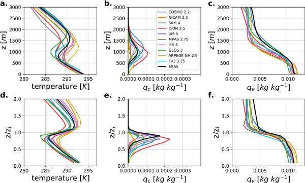
Figure 9a demonstrates that the mean free-tropospheric temperature differs by roughly 3 K between the coldest and the warmest model, whereas the MBL temperature is more similar due to the prescribed seasurface temperature. Free-tropospheric humidity (Fig. 9c) differs by 50 % between the driest and the wettest model and compared with ERA5 is underestimated in all of them. The underestimation implies that dryer air is entrained into the cloud layer, which may contribute to the overall underestimation of the low cloud cover. However, it seems unlikely that this is the dominant cause for the underestimation as the clouds differ from the start of the simulation, whereas the differences in the free troposphere develop during the course of the simulation. Models with a warmer free troposphere tend to have higher qv, which emphasizes the importance of where the air originates from (i.e., from the lower or higher latitudes). This is the opposite of what one would expect if the free-tropospheric temperature profile was strongly influenced by buoyancy changes due to humidity2. The qc-profiles (Fig. 9b) show that the lowest clouds have their base at very low heights, which is caused by cumulus cells forming below the stratocumulus decks (c.f. Fig. 8), whereas low-stratus clouds in the South-East of the domain may contribute (c.f. e.g., Zheng et al. 2018a). The largest amount of cloud water is located in the upper half of the MBL where the inversion sharply caps the clouds towards the top of the MBL (Fig. 9e). The cloud cover is largest between 60 % (ARPEGE 2.5) and 90 % (MPAS 3.75, IFS 4, and SAM 4) of the inversion height.
In coarser resolved climate models, it was found that models with higher qv within the MBL have lower free-tropospheric qv due to differences in vertical mixing between the MBL and the free troposphere (Sherwood et al. 2014). This is not the case for the simulations analyzed here as shown in the qv profiles (Figs. 9c, f). However, the models with a lower inversion (e.g., NICAM and ARPEGE-NH) have enhanced qv within the MBL compared with others, presumably because the drying of the MBL due to entrainment in these models is weaker (as will be shown later) and because turbulent fluxes can adjust the profiles more quickly.
Figure 10 presents profiles of the mean vertical wind and the standard deviation of the vertical wind (σw) to quantify the average strength of overturning convective circulations. σw is scaled by the local inversion height (see, e.g., Lilly 2002) in the relative profile (Fig. 10d) to obtain an expression that is independent of the local MBL depth (σw/zi). Figure 10a demonstrates that the mean vertical wind is negative at all levels, i.e., there is large-scale subsidence. The relative profile (Fig. 10c) reveals more systematic information about its vertical structure. Around the inversion, the downward motion increases sharply, reaching its peak just below the inversion and then gradually decreasing towards the surface. This implies that much of the divergence of the horizontal wind field is confined to the boundary layer. The comparison of Fig. 10c and Fig. 10d shows that models with on average stronger subsidence across the inversion tend to simulate stronger vertical convective mixing within the MBL.

In this section, we consider diabatic heating approximated according to (4). It is shown as a relative height profile together with qc in Figs. 11a, b. Furthermore, Figs. 11c, d present the potential temperature divergence (v · ∇θ) separated into the mean component (v̄ · ∇θ̄) and the eddy component ().

There is strong diabatic cooling around the MBL top (Fig. 11a) resulting from longwave emission and evaporation due to dry-air entrainment in the upper part of the cloud layer (e.g., Mellado 2017). This is compensated by enhanced large-scale subsidence and convergence of the horizontal wind field (Fig. 11c), as well as by turbulent entrainment of warm air at the inversion (Fig. 11d). The diabatic cooling in the free troposphere (relative height > 1.25) is weak and constant with height. It represents the longwave flux divergence due to greenhouse gases that drives the large-scale subsidence (Fig. 11c). The weak warming in the lower half of the MBL is interpreted as subgrid-scale turbulent heating from the surface sensible heat flux counteracting radiative cooling and coldair advection (Fig. 11c). In the lower half of the cloud layer (relative heights between 0.25 and 0.75), some models show enhanced diabatic heating that may be caused by radiative flux convergence at the cloud base.
Summarizing, Figs. 10, 11 present a mean downward motion across the inversion layer (Fig. 10c). The diabatic warming (Fig. 11a) thereby converts freetropospheric air into MBL air. The diabatic effects comprise a dipole between radiative cooling at the cloud top and condensational warming within the cloud layer, as well as turbulent heating and cooling. The net gain of mass below the inversion, defined as the entrainment (7), is then compensated by horizontal divergence, as we can assume quasi-steady conditions.
d. Entrainment at the top of the MBL
Following the previous findings, the entrainment velocity at the inversion is computed after (7). Figures 12a, b shows the co-variance between the mean inversion height and the entrainment. Models with stronger entrainment have higher inversions (SAM 4 is an exception to this relation with particularly strong entrainment). The same relation is observed in some models on the basis of daily mean values (Fig. 12b). Assuming steady-state conditions, entrainment has to be locally compensated by horizontal divergence below the inversion. If more air is entrained into the MBL, it grows more quickly against the suppression from the large-scale subsidence along its trajectory. The inter-model variability found for the inversion height (e.g., Fig. 6) can thus partly be explained in terms of differences in entrainment.

Figures 12c, d show a positive correlation between the entrainment and the surface latent heat flux. In a stratocumulus-topped MBL, we expect a larger latent heat flux when the entrainment is strong because the associated drying of the MBL enhances the saturation deficit of the near-surface air (Bretherton and Wyant 1997; Stevens 2007; Zheng et al. 2018b). The model simulations reproduce this behavior for daily mean values (Fig. 12d), indicating that the signal of the enhanced entrainment propagates to the surface. Also, in the inter-model comparison, the latent heat flux tends to be larger in models with stronger entrainment (Fig. 12c).
Finally, Figs. 12e, f show how the cloud field relates to the entrainment. Models with enhanced cloud cover have stronger entrainment, and this relation is visible also in the day-to-day variability in some models. Whether the amount of clouds controls the entrainment strength and/or vice versa cannot be said. From theory, in the stratocumulus-topped MBL, one would expect an increased cloud cover to maintain stronger radiative cooling at the inversion and thus favor entrainment. Stronger entrainment at the inversion is also going along with more vigorous convective circulations within the MBL (Figs. 10c, d). This would point towards a cloud layer that is better coupled to the surface, which would help sustain the positive relation between cloud cover and entrainment. The interpretation of these results requires some caution as the cloud composition should vary over the domain (stratocumulus vs. trade-wind cumulus clouds) and, in particular, the representation of this variation in the individual models. Additional analyzes using smaller sub-domains, however, revealed that the inter-model relation between entrainment and cloud cover is robust across the domain.
e. Sensitivity to turbulence formulation
As turbulence is essential for MBLs, we consider two sensitivity experiments with reduced turbulent length scale. The simulations are identical to COSMO 4.4 but use turbulent length scales of 50 m and 25 m, respectively (COSMO 4.4 tl50m, COSMO 4.4 tl25m). These simulations are shown in the left-hand panels of Figs. 7, 12. Weaker sub-grid-scale turbulent mixing results in a lower inversion and a reduction in cloud cover (Fig. 7a). The associated reduction is quite substantial, with COSMO 4.4 tl50m having a similar albedo to COSMO 2.2, thereby strongly reducing the resolution sensitivity exhibited by Figs. 2m, n. The impact of reduced turbulence goes along with weaker entrainment (Fig. 12a), a weaker latent heat flux (Fig. 12c), and a weaker inversion (Fig. 7c). Thus, even though the resolved vertical mixing in COSMO is stronger than in other models (see Fig. 10), sub-gridscale mixing plays a key role in the coupling between the cloud layer and the surface. This may also be the case in the other CRMs. Overall, changing the subgrid-scale turbulent mixing induces changes that qualitatively follow the inter-model variability of the CRM intercomparison fairly well.
4. Discussion
Considering only the members of the CRM intercomparison (2 km < Δx < 5 km), the inter-model variability in the cloud cover at these resolutions remains considerable. This is not too surprising as even LES studies find substantial inter-model spread for similar large-scale conditions (e.g., Stevens et al. 2005). The domain average albedo covers a range of approximately 0.2 or between 40 % and 110 % of the observed value. Based on the insights gained from these 10 simulations, the model characteristics appear significantly more important than the exact choice of resolution. There is no indication that simulations with resolutions 2 km < Δx < 3 km produce closer-to-observed albedo than those with resolutions 4 km < Δx < 5 km (roughly half resolution). We also find no systematic differences between the 5 models employing a shallow convection scheme (UM, IFS, MPAS, FV3, and GEOS) and the other 5 models (SAM, NICAM, ARPEGE-NH, ICON, and COSMO). Thus, it appears that whether or not a shallow convection scheme is employed is not the crucial factor determining the cloud amount in CRMs. However, the variety of shallow convection schemes employed is large, and a definite conclusion appears to be challenging.
The finding that simulations with a deeper MBL produce increased cloud cover may seem surprising. A too deep MBL leads to a dynamical decoupling of the cloud layer from the surface and favors the breakup of the stratocumulus decks into trade-wind cumuli. However, in a shallow MBL, entrainment can also help deepen the cloud layer (Randall 1984), and the associated deepening of the MBL reduces the saturation deficit of the near-surface air increasing the latent heat flux (e.g., Hourdin et al. 2015). This implies that getting the depth of the MBL right appears to be crucial for a realistic representation of cloud cover. Based on the insights gained here, the models with a too shallow MBL and weak entrainment and convective mixing thus show a physically consistent response, which, however, results in too little cloud cover.
What ultimately controls the amount of clouds in the analyzed models remains a challenging question. Differences in the cloud top radiative cooling may be relevant by controlling the generation of negative buoyancy (e.g., Hoffmann et al. 2020). Another potential cause is that the choices of model architecture and tuning parameters may result in different effective strengths of the convective and turbulent mixing, which controls the entrainment rate, the MBL depth, and the moisture supply of the stratocumulus layer. The sensitivity experiments performed with the COSMO model provide support for this hypothesis. Weaker sub-grid-scale turbulent mixing leads to changes that agree well with the inter-model differences in entrainment, MBL depth, and the latent heat flux. Conversely, in the 5 COSMO simulations with identical turbulent length scale but decreasing horizontal grid spacing from 12 km down to 0.5 km, the cloud cover changes strongly as a function of resolution. The albedo is reduced by 0.25 between COSMO 12 and COSMO 0.5 going along with a weaker inversion. The MBL depth, however, is virtually the same in these simulations, and also the entrainment and the latent heat flux are similar. Further work to improve the understanding of the cloud cover's sensitivity to horizontal resolution is the goal of ongoing work.
Our study has a number of limitations. First of all, as the simulations are only 40 days long, and as the global models exhibit substantial internal variability, a direct comparison of inter-model variations is challenging. However, we find that most of the characteristics of each model emerge within 1–2 days, at a time when the large-scale circulation is predictable. Another challenging issue is the aerosol effects. Over the analyzed region, the aerosol load can be high due to biomass burning (Zuidema et al. 2016), which could, in principle, also affect the inter-model variability in cloud cover. This effect is difficult to assess, as it depends on the specific treatment of aerosols and microphysics in each model.
5. Conclusion
We used data from the DYAMOND project and performed COSMO model simulations to conduct a model intercomparison using 10 convection-resolving models (CRMs; 5-km to 2-km resolution), as well as a resolution intercomparison (12-km to 0.5-km resolution) with one single model (COSMO) over 40 days on a domain covered by tropical and subtropical low clouds. The main results are summarized as follows:
-
• Most models quite realistically simulate the low cloud field but underestimate the albedo. Differences between models and observations can be attributed to a too low cloud fraction and/or a too low cloud albedo, depending on the model.
-
• The sharp gradient of atmospheric fields across the inversion is represented well in the simulations. All models simulate a domain average inversion strength of approximately 8–12 K, resulting in a strong capping of the cloud layer. The mean vertical distribution of subsidence and diabatic heating is qualitatively comparable in all models.
-
Ȃ All models overestimate outgoing longwave radiation (OLR) by 6–16 W m−2 which can be explained not only by underestimated free-tropospheric humidity but also by too few low clouds. Free tropospheric humidity varies by up to 50 % between the models and is underestimated by all of them.
-
• The average depth of the MBL differs considerably among the analyzed models partly as a consequence of different entrainment rates. In models with stronger entrainment, the MBL grows deeper along the trade winds, leading to a higher-average MBL depth. These models also tend to simulate more vigorous MBL dynamics and an increased surface latent heat flux, all of which is typical for the stratocumulus-topped MBL.
-
• On average, the models with stronger entrainment produce enhanced low cloud cover–or vice versa. Grid-scale convective mixing within the MBL is stronger in these models, which suggests a better coupled MBL that can feed more moisture into the cloud layer. However, sensitivity simulations with the COSMO model also highlight the importance of sub-grid-scale turbulent mixing.
-
• The resolution intercomparison with the COSMO model shows that there are strong reductions in cloud cover when refining the resolution from 12 km to 4 km, whereas the sensitivity between 4 km and 500 m becomes much smaller, even though the model was not calibrated for the respective resolutions. This suggests that the latter range is attractive for climate studies.
Overall, the inter-model spread found in this study implies that low clouds remain a challenging topic even in CRMs. Still, our results are encouraging as they shed light on the benefits of using CRMs to simulate low clouds. First, from a visual point of view, most models show a cloud field that is characterized by the type of cloud structures that we expect to see in reality. This indicates that some of the fundamental meso-scale dynamical interactions, for instance, cold pool dynamics, start to act, consistent with the findings of previous CRM studies (e.g., Leutwyler et al. 2016; Klocke et al. 2017). Second, the inter-model variability in the cloud cover systematically relates to the variability in other properties of the MBL–such as entrainment, inversion height, and the latent heat flux. Third, sensitivity experiments with the COSMO model demonstrate that the strength of sub-grid-scale turbulent mixing can strongly affect the aforementioned relations. Overall, this points to the vertical mixing schemes as a key parameterization problem and outlines the potential of model calibration to improve the models' performance in comparison with the observations. Doing so may lead to an overall more consistent representation of the MBL due to the systematic response of the models. This parameterization problem should be solvable, certainly more tractable than the existing compound parameterization problems we face in coarser climate models with parameterized convection (e.g., Teixeira et al. 2011; Zhang et al. 2013; Qu et al. 2014; Vial et al. 2016).
Acknowledgments
The authors want to thank 3 anonymous reviewers and the editor for their constructive and valuable feedback, which helped a lot in revising the study. The main author also wants to express his thanks to Shweta Singh for the inspiring collaboration at the DYAMOND Hackathon in Mainz in June 2019 which was an ideal starting point for this work.
This work was partly funded by the Swiss National Science Foundation (SNSF) project “Exploiting km-resolution climate models in the tropics to constrain climate change uncertainties” (trCLIM) and partly by the EU-funded project “Constraining uncertainty of multi-decadal climate projections” (CONSTRAIN).
We are indebted to the Partnership for Advanced Computing in Europe (PRACE) for granting us access to the supercomputer Piz Daint at the Swiss National Supercomputing Centre (CSCS), Switzerland. We also acknowledge the Federal Office for Meteorology and Climatology MeteoSwiss, CSCS, and ETH Zürich for their contributions to the development of the GPU-accelerated version of COSMO.
Concerning the external data sets used in this study, we are grateful for the ERA5 reanalysis data set provided by the European Centre for Medium-Range Weather Forecasts (ECMWF). Finally, we would like to thank the contributors of the DYAMOND project for providing this valuable data. The DYAMOND data storage was provided by the German Climate Computing Centre (DKRZ) and facilitated through the projects ESiWACE and ESiWACE2. The projects ESiWACE and ESiWACE2 have received funding from the European Union's Horizon 2020 research and innovation programme under grant agreements No. 675191 and 823988.
The authors declare no conflict of interest.
Footnotes
1https://www.esiwace.eu/services/dyamond, accessed on 3 June 2020.
2Since the weight of air decreases with moisture load, intermodel differences in free-tropospheric humidity contribute to temperature differences as the atmospheric profile adjusts to the buoyancy changes. The inter-model spread in qv of roughly 2 g kg−1 at 3-km height can, however, explain a temperature difference of only 0.4 K.
References
- Ackerman, A. S., M. C. Van Zanten, B. Stevens, V. Savic-Jovcic, C. S. Bretherton, A. Chlond, J.-C. Golaz, H. Jiang, M. Khairoutdinov, S. K. Krueger, D. C. Lewellen, A. Lock, C.-H. Moeng, K. Nakamura, M. D. Petters, J. R. Snider, S. Weinbrecht, and M. Zulauf, 2009: Large-eddy simulations of a drizzling, stratocumulus-topped marine boundary layer. Mon. Wea. Rev., 137, 1083-1110.
- Arnold, N. P., W. M. Putman, and S. R. Freitas, 2020: Impact of resolution and parameterized convection on the diurnal cycle of precipitation in a global non-hydrostatic model. J. Meteor. Soc. Japan, 98, 1279-1304.
- Baldauf, M., and G. Zängl, 2012: Horizontal nonlinear Smagorinsky diffusion. COSMO Newsl., 2, 3-7.
- Ban, N., J. Schmidli, and C. Schär, 2014: Evaluation of the convection-resolving regional climate modeling approach in decade-long simulations. J. Geophys. Res.: Atmos., 119, 7889-7907.
- Bony, S., and J.-L. Dufresne, 2005: Marine boundary layer clouds at the heart of tropical cloud feedback uncertainties in climate models. Geophys. Res. Lett., 32, L20806, doi:10.1029/2005GL023851.
- Bony, S., B. Stevens, D. M. W. Frierson, C. Jakob, M. Kageyama, R. Pincus, T. G. Shepherd, S. C. Sherwood, A. P. Siebesma, A. H. Sobel, M. Watanabe, and M. J. Webb, 2015: Clouds, circulation and climate sensitivity. Nat. Geosci., 8, 261-268.
- Bott, A., 1989: A positive definite advection scheme obtained by non-linear renormalization of the advective fluxes. Mon. Wea. Rev., 117, 1006-1016.
- Boucher, O., D. Randall, P. Artaxo, C. Bretherton, G. Feingold, P. Forster, V.-M. Kerminen, Y. Kondo, H. Liao, U. Lohmann, P. Rasch, S. K. Satheesh, S. Sherwood, B. Stevens, and X.-Y. Zhang, 2013: Clouds and aerosols. Climate Change 2013: The Physical Science Basis. Contribution of Working Group I to the Fifth Assessment Report of the Intergovernmental Panel on Climate Change. Stocker, T. F., D. Qin, G.-K. Plattner, M. Tignor, S. K. Allen, J. Boschung, A. Nauels, Y. Xia, V. Bex, and P. M. Midgley (eds.), Cambridge University Press, Cambridge, UK and New York, USA, 571-657.
- Bretherton, C. S., and M. C. Wyant, 1997: Moisture transport, lower-tropospheric stability, and decoupling of cloud-topped boundary layers. J. Atmos. Sci., 54, 148-167.
- Bretherton, C. S., and M. F. Khairoutdinov, 2015: Convective self-aggregation feedbacks in near-global cloudresolving simulations of an aquaplanet. J. Adv. Model. Earth Syst., 7, 1765-1787.
- Brient, F., T. Schneider, Z. Tan, S. Bony, X. Qu, and A. Hall, 2016: Shallowness of tropical low clouds as a predictor of climate models' response to warming. Climate Dyn., 47, 433-449.
- Cao, C., F. J. De Luccia, X. Xiong, R. Wolfe, and F. Weng, 2014: Early on-orbit performance of the visible infrared imaging radiometer suite onboard the Suomi National Polar-orbiting Partnership (S-NPP) satellite. IEEE Trans. Geosci. Remote Sens., 52, 1142-1156.
- Charney, J. G., A. Arakawa, D. J. Baker, B. Bolin, R. E. Dickinson, R. M. Goody, C. E. Leith, H. M. Stommel, and C. I. Wunsch, 1979: Carbon dioxide and climate: A scientific assessment. Report of an ad hoc study group on carbon dioxide and climate. National Research Council, Washington, D.C., 20 pp.
- Collins, M., R. Knutti, J. Arblaster, J.-L. Dufresne, T. Fichefet, P. Friedlingstein, X. Gao, W. J. Gutowski, Jr., T. Johns, G. Krinner, M. Shongwe, C. Tebaldi, A. J. Weaver, and M. Wehner, 2013: Long-term climate change: Projections, commitments and irreversibility. Climate Change 2013: The Physical Science Basis. Contribution of Working Group I to the Fifth Assessment Report of the Intergovernmental Panel on Climate Change. Stocker, T. F., D. Qin, G.-K. Plattner, M. Tignor, S. K. Allen, J. Boschung, A. Nauels, Y. Xia, V. Bex, and P. M. Midgley (eds.), Cambridge University Press, Cambridge, UK and New York, USA, 1029-1136.
- Copernicus Climate Change Service (C3S), 2017: ERA5: Fifth generation of ECMWF atmospheric reanalyses of the global climate. Copernicus Climate Change Service Climate Data Store (CDS). [Available at https://cds.climate.copernicus.eu/cdsapp#!/home.]
- Courcoux, N., and M. Schröder, 2015: The CM SAF ATOVS data record: Overview of methodology and evaluation of total column water and profiles of tropospheric humidity. Earth Syst. Sci. Data, 7, 397-414.
- de Roode, S. R., and C. S. Bretherton, 2003: Mass-flux budgets of shallow cumulus clouds. J. Atmos. Sci., 60, 137-151.
- Deardorff, J. W., 1980: Cloud top entrainment instability. J. Atmos. Sci., 37, 131-147.
- Dueben, P. D., N. Wedi, S. Saarinen, and C. Zeman, 2020: Global simulations of the atmosphere at 1.45 km grid-spacing with the Integrated Forecasting System. J. Meteor. Soc. Japan, 98, 551-572.
- Fuhrer, O., C. Osuna, X. Lapillonne, T. Gysi, B. Cumming, M. Bianco, A. Arteaga, and T. C. Schulthess, 2014: Towards a performance portable, architecture agnostic implementation strategy for weather and climate models. Supercomput. Front. Innovations, 1, 44-61.
- Fuhrer, O., T. Chadha, T. Hoefler, G. Kwasniewski, X. Lapillonne, D. Leutwyler, D. Lüthi, C. Osuna, C. Schär, T. C. Schulthess, and H. Vogt, 2018: Nearglobal climate simulation at 1 km resolution: Establishing a performance baseline on 4888 GPUs with COSMO 5.0. Geosci. Model Dev., 11, 1665-1681.
- Heise, E., M. Lange, B. Ritter, and R. Schrodin, 2003: Improvement and validation of the multilayer soil model. COSMO Newsl., 3, 198-203.
- Heus, T., and A. Seifert, 2013: Automated tracking of shallow cumulus clouds in large domain, long duration large eddy simulations. Geosci. Model Dev., 6, 1261-1273.
- Hoffmann, F., F. Glassmeier, T. Yamaguchi, and G. Feingold, 2020: Liquid water path steady states in stratocumulus: Insights from process-level emulation and mixed-layer theory. J. Atmos. Sci., 77, 2203-2215.
- Hohenegger, C., L. Kornblueh, D. Klocke, T. Becker, G. Cioni, J. F. Engels, U. Schulzweida, and B. Stevens, 2020: Climate statistics in global simulations of the atmosphere, from 80 to 2.5 km grid spacing. J. Meteor. Soc. Japan, 98, 73-91.
- Hourdin, F., A. Găinusă-Bogdan, P. Braconnot, J.-L. Dufresne, A.-K. Traore, and C. Rio, 2015: Air moisture control on ocean surface temperature, hidden key to the warm bias enigma. Geophys. Res. Lett., 42, 10885-10893.
- Ito, J., S. Hayashi, A. Hashimoto, H. Ohtake, F. Uno, H. Yoshimura, T. Kato, and Y. Yamada, 2017: Stalled improvement in a numerical weather prediction model as horizontal resolution increases to the sub-kilometer scale. SOLA, 13, 151-156.
- Jaeger, E. B., I. Anders, D. Lüthi, B. Rockel, C. Schär, and S. I. Seneviratne, 2008: Analysis of ERA40-driven CLM simulations for Europe. Meteor. Z., 17, 349-367.
- Klemp, J. B., and R. B. Wilhelmson, 1978: The simulation of three-dimensional convective storm dynamics. J. Atmos. Sci., 35, 1070-1096.
- Klocke, D., M. Brueck, C. Hohenegger, and B. Stevens, 2017: Rediscovery of the doldrums in storm-resolving simulations over the tropical Atlantic. Nat. Geosci., 10, 891-896.
- Leutwyler, D., O. Fuhrer, X. Lapillonne, D. Lüthi, and C. Schär, 2016: Towards European-scale convection-resolving climate simulations with GPUs: A study with COSMO 4.19. Geosci. Model Dev., 9, 3393-3412.
- Lilly, D. K., 1968: Models of cloud-topped mixed layers under a strong inversion. Quart. J. Roy. Meteor. Soc., 94, 292-309.
- Lilly, D. K., 2002: Entrainment into mixed layers. Part I: Sharp-edged and smoothed tops. J. Atmos. Sci., 59, 3340-3352.
- Mellado, J. P., 2017: Cloud-top entrainment in stratocumulus clouds. Annu. Rev. Fluid Mech., 49, 145-169.
- Miyamoto, Y., Y. Kajikawa, R. Yoshida, T. Yamaura, H. Yashiro, and H. Tomita, 2013: Deep moist atmospheric convection in a subkilometer global simulation. Geophys. Res. Lett., 40, 4922-4926.
- Nam, C., S. Bony, J.-L. Dufresne, and H. Chepfer, 2012: The ‘too few, too bright’ tropical low-cloud problem in CMIP5 models. Geophys. Res. Lett., 39, 1-7.
- Neiburger, M., D. S. Johnson, and C.-W. Chien, 1961: Studies of the Structure of the Atmosphere over the Eastern Pacific Ocean in Summer: Part 1. The Inversion Over the Eastern North Pacific Ocean. University of California Publ. in Meteorology, 94 pp.
- Nicholls, S., 1984: The dynamics of stratocumulus: Aircraft observations and comparisons with a mixed layer model. Quart. J. Roy. Meteor. Soc., 110, 783-820.
- Noda, A. T., and M. Satoh, 2014: Intermodel variances of subtropical stratocumulus environments simulated in CMIP5 models. Geophys. Res. Lett., 41, 7754-7761.
- Noda, A. T., K. Nakamura, T. Iwasaki, and M. Satoh, 2013: A numerical study of a stratocumulus-topped boundary-layer: Relations of decaying clouds with a stability parameter across inversion. J. Meteor. Soc. Japan, 91, 727-746.
- Nuijens, L., and A. P. Siebesma, 2019: Boundary layer clouds and convection over subtropical oceans in our current and in a warmer climate. Curr. Climate Change Rep., 5, 80-94.
- Possner, A., E. Zubler, O. Fuhrer, U. Lohmann, and C. Schär, 2014: A case study in modeling low-lying inversions and stratocumulus cloud cover in the Bay of Biscay. Wea. Forecasting, 29, 289-304.
- Prein, A. F., W. Langhans, G. Fosser, A. Ferrone, N. Ban, K. Goergen, M. Keller, M. Tölle, O. Gutjahr, F. Feser, E. Brisson, S. Kollet, J. Schmidli, N. P. M. van Lipzig, and R. Leung, 2015: A review on regional convection-permitting climate modeling: Demonstrations, prospects, and challenges. Rev. Geophysi., 53, 323-361.
- Qu, X., A. Hall, S. A. Klein, and P. M. Caldwell, 2014: On the spread of changes in marine low cloud cover in climate model simulations of the 21st century. Climate Dyn., 42, 2603-2626.
- Randall, D. A., 1984: Stratocumulus cloud deepening through entrainment. Tellus A, 36, 446-457.
- Raschendorfer, M., 2001: The new turbulence parameterization of LM. COSMO Newsl., 1, 89-97.
- Reinhardt, T., and A. Seifert, 2006: A three-category ice scheme for LMK. COSMO Newsl., 6, 115-120.
- Ritter, B., and J.-F. Geleyn, 1992: A comprehensive radiation scheme for numerical weather prediction models with potential applications in climate simulations. Mon. Wea. Rev., 120, 303-325.
- Rockel, B., A. Will, and A. Hense, 2008: The regional climate model COSMO-CLM (CCLM). Meteor. Z., 17, 347-348.
- Romps, D. M., 2017: Exact expression for the lifting condensation level. J. Atmos. Sci., 74, 3891-3900.
- Satoh, M., B. Stevens, F. Judt, M. Khairoutdinov, S.-J. Lin, W. M. Putman, and P. Düben, 2019: Global cloud-resolving models. Curr. Climate Change Rep., 5, 172-184.
- Schär, C., O. Fuhrer, A. Arteaga, N. Ban, C. Charpilloz, S. Di Girolamo, L. Hentgen, T. Hoefler, X. Lapillonne, D. Leutwyler, K. Osterried, D. Panosetti, S. Rüdisühli, L. Schlemmer, T. C. Schulthess, M. Sprenger, S. Ubbiali, and H. Wernli, 2020: Kilometer-scale climate models: Prospects and challenges. Bull. Amer. Meteor. Soc., 101, E567-E587.
- Schlemmer, L., C. Schär, D. Lüthi, and L. Strebel, 2018: A groundwater and runoff formulation for weather and climate models. J. Adv. Model. Earth Syst., 10, 1809-1832.
- Schneider, T., J. Teixeira, C. S. Bretherton, F. Brient, K. G. Pressel, C. Schär, and A. P. Siebesma, 2017: Climate goals and computing the future of clouds. Nat. Climate Change, 7, 3-5.
- Seifert, A., and T. Heus, 2013: Large-eddy simulation of organized precipitating trade wind cumulus clouds. Atmos. Chem. Phys., 13, 5631-5645.
- Sherwood, S. C., S. Bony, and J.-L. Dufresne, 2014: Spread in model climate sensitivity traced to atmospheric convective mixing. Nature, 505, 37-42.
- Sherwood, S. C., M. J. Webb, J. D. Annan, K. C. Armour, P. M. Forster, J. C. Hargreaves, G. Hegerl, S. A. Klein, K. D. Marvel, E. J. Rohling, M. Watanabe, T. Andrews, P. Braconnot, C. S. Bretherton, G. L. Foster, Z. Hausfather, A. S. Heydt, R. Knutti, T. Mauritsen, J. R. Norris, C. Proistosescu, M. Rugenstein, G. A. Schmidt, K. B. Tokarska, and M. D. Zelinka, 2020: An assessment of Earth's climate sensitivity using multiple lines of evidence. Rev. Geophys., 58, e2019RG000678, doi:10.1029/2019RG000678.
- Soden, B. J., and I. M. Held, 2006: An assessment of climate feedbacks in coupled ocean-atmosphere models. J. Climate, 19, 3354-3360.
- Stephens, G. L., 1978: Radiation profiles in extended water clouds. II: Parameterization schemes. J. Atmos. Sci., 35, 2123-2132.
- Steppeler, J., G. Doms, U. Schättler, H. W. Bitzer, A. Gassmann, U. Damrath, and G. Gregoric, 2003: Mesogamma scale forecasts using the nonhydrostatic model LM. Meteor. Atmos. Phys., 82, 75-96.
- Stevens, B., 2006: Bulk boundary-layer concepts for simplified models of tropical dynamics. Theor. Comput. Fluid Dyn., 20, 279-304.
- Stevens, B., 2007: On the growth of layers of nonprecipitating cumulus convection. J. Atmos. Sci., 64, 2916-2931.
- Stevens, B., C.-H. Moeng, A. S. Ackerman, C. S. Bretherton, A. Chlond, S. de Roode, J. Edwards, J.-C. Golaz, H. Jiang, M. Khairoutdinov, M. P. Kirkpatrick, D. C. Lewellen, A. Lock, F. Müller, D. E. Stevens, E. Whelan, and P. Zhu, 2005: Evaluation of large-eddy simulations via observations of nocturnal marine stratocumulus. Mon. Wea. Rev., 133, 1443-1462.
- Stevens, B., S. C. Sherwood, S. Bony, and M. J. Webb, 2016: Prospects for narrowing bounds on Earth's equilibrium climate sensitivity. Earth's Future, 4, 512-522.
- Stevens, B., M. Satoh, L. Auger, J. Biercamp, C. S. Bretherton, X. Chen, P. Düben, F. Judt, M. Khairoutdinov, D. Klocke, C. Kodama, L. Kornblueh, S.-J. Lin, P. Neumann, W. M. Putman, N. Röber, R. Shibuya, B. Vanniere, P. L. Vidale, N. Wedi, and L. Zhou, 2019: DYAMOND: The DYnamics of the Atmospheric general circulation Modeled On Non-hydrostatic Domains. Prog. Earth Planet. Sci., 6, 61, doi:10.1186/s40645-019-0304-z.
- Stevens, B., C. Acquistapace, A. Hansen, R. Heinze, C. Klinger, D. Klocke, H. Rybka, W. Schubotz, J. Windmiller, P. Adamidis, I. Arka, V. Barlakas, J. Biercamp, M. Brueck, S. Brune, S. A. Buehler, U. Burkhardt, G. Cioni, M. Costa-surós, S. Crewell, T. Crüger, H. Deneke, P. Friederichs, C. C. Henken, C. Hohenegger, M. Jacob, F. Jakub, N. Kalthoff, M. Köhler, T. W. van Laar, P. Li, U. Löhnert, A. Macke, N. Madenach, B. Mayer, C. Nam, A. K. Naumann, K. Peters, S. Poll, J. Quaas, N. Röber, N. Rochetin, L. Scheck, V. Schemann, S. Schnitt, A. Seifert, F. Senf, M. Shapkalijevski, C. Simmer, S. Singh, O. Sourdeval, D. Spickermann, J. Strandgren, O. Tessiot, N. Vercauteren, J. Vial, A. Voigt, and G. Zängl, 2020: The added value of large-eddy and storm-resolving models for simulating clouds and precipitation. J. Meteor. Soc. Japan, 98, 395-435.
- Stöckli, R., A. Duguay-Tetzlaff, J. Bojanowski, R. Hollmann, P. Fuchs, and M. Werscheck, 2017: CM SAF ClOud Fractional Cover dataset from METeosat First and Second Generation - Edition 1 (COMET Ed. 1). EUMETSAT, Darmstadt, Germany. doi:10.5676/EUM_SAF_CM/CFC_METEOSAT/V001.
- Teixeira, J., S. Cardoso, M. Bonazzola, J. Cole, A. DelGenio, C. DeMott, C. Franklin, C. Hannay, C. Jakob, Y. Jiao, J. Karlsson, H. Kitagawa, M. Köhler, A. Kuwano-Yoshida, C. LeDrian, J. Li, A. Lock, M. J. Miller, P. Marquet, J. Martins, C. R. Mechoso, E. v. Meijgaard, I. Meinke, P. M. A. Miranda, D. Mironov, R. Neggers, H. L. Pan, D. A. Randall, P. J. Rasch, B. Rockel, W. B. Rossow, B. Ritter, A. P. Siebesma, P. M. M. Soares, F. J. Turk, P. A. Vaillancourt, A. von Engeln, and M. Zhao, 2011: Tropical and subtropical cloud transitions in weather and climate prediction models: The GCSS/WGNE Pacific cross-section intercomparison (GPCI). J. Climate, 24, 5223-5256.
- Urbain, M., N. Clerbaux, A. Ipe, F. Tornow, R. Hollmann, E. Baudrez, A. Velazquez Blazquez, and J. Moreels, 2017: The CM SAF TOA radiation data record using MVIRI and SEVIRI. Remote Sens., 9, 466, doi:10.3390/rs9050466.
- Vergara-Temprado, J., A. K. Miltenberger, K. Furtado, D. P. Grosvenor, B. J. Shipway, A. A. Hill, J. M. Wilkinson, P. R. Field, B. J. Murray, and K. S. Carslaw, 2018: Strong control of Southern Ocean cloud reflectivity by ice-nucleating particles. Proc. Natl. Acad. Sci. U.S.A. (PNAS), 115, 2687-2692.
- Vergara-Temprado, J., N. Ban, D. Panosetti, L. Schlemmer, and C. Schär, 2020: Climate models permit convection at much coarser resolutions than previously considered. J. Climate, 33, 1915-1933.
- Vial, J., S. Bony, J.-L. Dufresne, and R. Roehrig, 2016: Coupling between lower-tropospheric convective mixing and low-level clouds: Physical mechanisms and dependence on convection scheme. J. Adv. Model. Earth Syst., 8, 1892-1911.
- Warren, S. G., C. J. Hahn, J. London, R. M. Chervin, and R. L. Jenne, 1986: Global distribution of total cloud cover and cloud type amounts over land. NCAR Technical report, NCAR/TN-273+STR, USDOE Office of Energy Research (ER), 230 pp.
- Warren, S. G., C. H. Hahn, J. London, R. M. Chervin, and R. L. Jenne, 1988: Global distribution of total cloud cover and cloud type amounts over the ocean. NCAR Technical Notes, NCAR/TN-317+STR, USDOE Office of Energy Research and National center for Atmospheric Research, USA, 350 pp.
- Wicker, L. J., and W. C. Skamarock, 2002: Time-splitting methods for elastic models using forward time schemes. Mon. Wea. Rev., 130, 2088-2097.
- Wood, R., 2012: Stratocumulus clouds. Mon. Wea. Rev., 140, 2373-2423.
- Wyant, M. C., C. S. Bretherton, H. A. Rand, and D. E. Stevens, 1997: Numerical simulations and a conceptual model of the stratocumulus to trade cumulus transition. J. Atmos. Sci., 54, 168-192.
- Zelinka, M. D., C. Zhou, and S. A. Klein, 2016: Insights from a refined decomposition of cloud feedbacks. Geophys. Res. Lett., 43, 9259-9269.
- Zelinka, M. D., T. A. Myers, D. T. McCoy, S. Po-Chedley, P. M. Caldwell, P. Ceppi, S. A. Klein, and K. E. Taylor, 2020: Causes of higher climate sensitivity in CMIP6 models. Geophys. Res. Lett., 47, e2019GL085782, doi:10.1029/2019GLL085782.
- Zhang, M., C. S. Bretherton, P. N. Blossey, P. H. Austin, J. T. Bacmeister, S. Bony, F. Brient, S. K. Cheedela, A. Cheng, A. D. Del Genio, S. R. De Roode, S. Endo, C. N. Franklin, J.-C. Golaz, C. Hannay, T. Heus, F. A. Isotta, J.-L. Dufresne, I.-S. Kang, H. Kawai, M. Köhler, V. E. Larson, Y. Liu, A. P. Lock, U. Lohmann, M. F. Khairoutdinov, A. M. Molod, R. A. J. Neggers, P. Rasch, I. Sandu, R. Senkbeil, A. P. Siebesma, C. Siegenthaler-Le Drian, B. Stevens, M. J. Suarez, K.-M. Xu, K. von Salzen, M. J. Webb, A. Wolf, and M. Zhao, 2013: CGILS: Results from the first phase of an international project to understand the physical mechanisms of low cloud feedbacks in single column models. J. Adv. Model. Earth Syst., 5, 826-842.
- Zheng, Y., D. Rosenfeld, and Z. Li, 2018a: Estimating the decoupling degree of subtropical marine stratocumulus decks from satellite. Geophys. Res. Lett., 45, 12560-12568.
- Zheng, Y., D. Rosenfeld, and Z. Li, 2018b: The relationships between cloud top radiative cooling rates, surface latent heat fluxes, and cloud-base heights in marine stratocumulus. J. Geophys. Res.: Atmos., 123, 11678-11690.
- Zuidema, P., J. Redemann, J. Haywood, R. Wood, S. Piketh, M. Hipondoka, and P. Formenti, 2016: Smoke and clouds above the southeast Atlantic: Upcoming field campaigns probe absorbing aerosol's impact on climate. Bull. Amer. Meteor. Soc., 97, 1131-1135.


