1. INTRODUCTION
Road asset management (RAM) is a type of social infrastructure asset management that is applied to road assets, such as roads, bridges, and other road components. The main purpose of this concept is to implement a strategic management plan to minimize the life cycle cost of road assets through the action of regular inspection, degradation forecast, and implementation of suitable repair activities at the best time.
The implementation of RAM in Nepal can be traced to the Rana Regime (1846-1951). The road office named ’Bato Kaj Goshwara’ for road construction and ’Chhembhadel Adda’ for maintenance works was established which was later transformed into public work directive after the advent of democracy in 1951. Department of Roads (DOR) was separated from the public work directive in 1962 and established as a service-oriented institution responsible for the construction and maintenance of Strategic Road Networks (SRNs) in Nepal1).
At present Nepal has 33,716 Km of road network constructed and maintained by various road agencies (RA) like the DOR, Department of Local Infrastructure, Department of Urban Development and Building Construction, municipalities, etc2). The DOR is identified as the key RA for the construction and maintenance of SRN. SRN includes the National Highway, Feeder Roads, and Sub Urban Road Network of a total length of 14,656 km and 1,656 numbers of bridges excluding the underconstruction and planned highway of approximately 3,536 km3),4). DOR Strategy, July 1995 highlights the departmental policy document that was developed with the strategies to attain the end goal - "the reduction of total road transport cost". This departmental end goal was also incorporated by the National Planning Commission into the 8th National Plan (1991/92). The total road transport costs are the sum of independent costs of road construction, road maintenance, and vehicle operating costs5)5). The comprehensive guideline of maintenance activities adopted by DOR to preserve the road in a serviceable state for road users and defer the need for highcost road maintenance activities are well described in policy documents6).
The annual budget for SRN maintenance is allocated by the Roads Board Nepal (RBN). The road board fund is composed of direct road toll collected from the road user, fuel levy, and vehicle registration fee7). There are four major performance measurements: i) surface roughness ii) surface distress iii) structural capacity and iv) pavement texture are suggested to determine how well the pavement is performing and meeting the serviceability of the road8).
Under the funding of RBN, the DOR has been collecting inspection data for International Roughness Index (IRI), Surface Distress Index (SDI), and Annual Average Daily Traffic (AADT) yearly. The traffic Survey involved traffic counting and analysis from 160 stations which are at the major nodal locations on the strategic road network of Nepal. Based on these data, the simple empirical method developed in 2005 is used to prepare the integrated annual road maintenance plan for all road division offices9). The Planned maintenance and the detailed methodology for the selection of the roads are explained in "Standard Procedure for Periodic Maintenance Planning", published in November 2005 in which the key pavement performance parameter considered is SDI9). The annual road condition survey conducted for SDI in 2023 indicates 58.4 percent of the bituminous roads are in fair to good condition (SDI range 0.0-3.0)3).
SDI is a measurement of pavement distress such as cracks, potholes, rutting and other forms of pavement deterioration. Highway engineers and pavement experts conduct visual surveys and record the severity of the distress. This data is used to calculate the SDI value for the surveyed road section. The methodology and interpretation of the results may vary depending on the surveyors and the guidelines of the road agencies. In context of Nepal, SDI surveys are done manually by trained highway engineers. Pavement surface distress is visually assessed by using a 10% sampling procedure and recorded. SDI is expressed in rating scale from 0 to 5. The rating 0 indicates a pavement surface without any defects, whereas a rating of 5 indicates the maximum possible deterioration. This method adopted by DOR is a simplified procedure recommended by the World Bank which has been modified to suit the conditions in Nepal and the need for DOR. Detail procedure for the determination of SDI value for each road link is described in "Road Pavement Management, MRCU"8).
On the other hand, IRI is an internationally recognized standard for assessing road roughness. It is expressed in m/km. The standard procedure and roughness measuring devices are standardized by World Bank sponsored International Road Roughness Experiments conducted in Brazil in 198210). The results are consistent and can be compared with other road sections locally and globally. The results of IRI can be correlated with ride quality and road user satisfaction.
DOR is facing the challenge of achieving one of its important maintenance policies to maintain over 95 percent of SRN in fair to good condition. In the future aging road infrastructure and an increase in traffic volume will add up more difficulties to achieving this target. Timely predictions on maintenance demands of the road assets in the future along with the appropriate financial plans to implement the optimal repair strategy are important to overcome this challenge. In addition, the rate of deterioration of the road pavement is important for planning the appropriate maintenance approach. However, the pavement deterioration curve for the condition of Nepal is not available to forecast future deterioration.
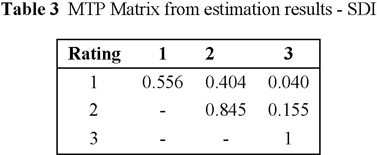
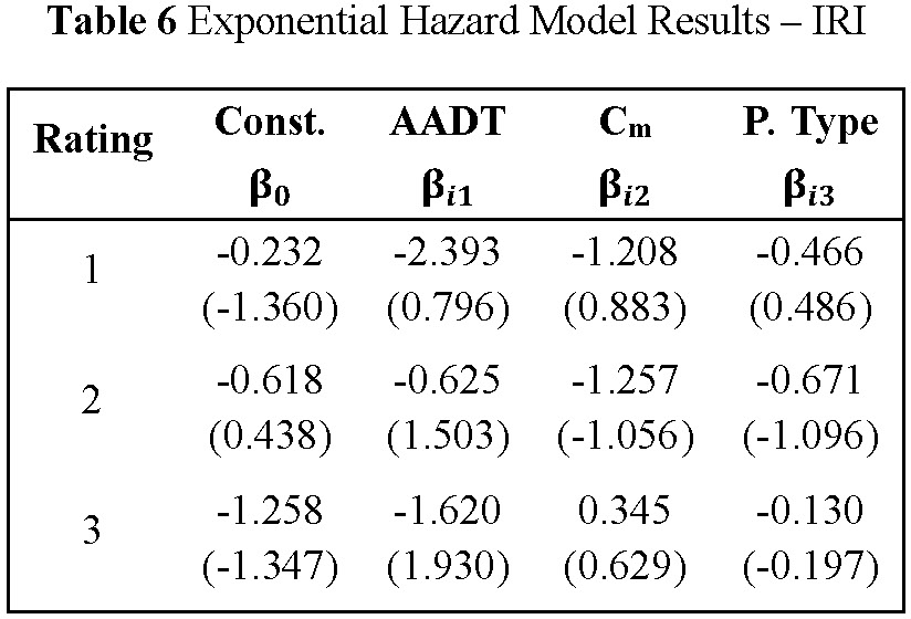
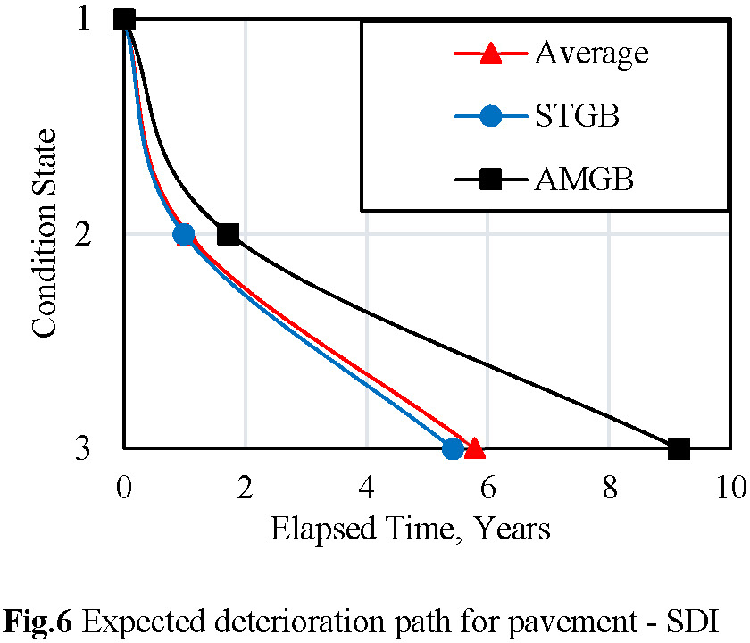
In this study, the Markov deterioration hazard model is applied for deterioration forecasting of SRN using road condition data set from 2014 to 2023 using two different performance parameters, SDI and IRI. The deterioration model can be applied to estimate the hazard rates and residual life of the pavement. Further, the average Markov transition probabilities (MTP) matrix, the hazard rate for each transition state, the life expectancy, and the expected deterioration path describing the average deterioration process during the life expectancy rating is presented in this paper.
2. METHODOLOGY
To forecast the deterioration progress of the pavement a statistical deterioration model based on past inspection results is applied. The Markov deterioration hazard model is a statistical model used to forecast the deterioration progress of pavement developed by Tsuda et al., 200611). In this model, a rank order is assigned as a condition state depending on the result of the past inspection data. The MTP are estimated to represent the deterioration progress between the condition states. This model is widely preferred for sound maintenance strategies and budget management policies. In this paper, the application of the Markov deterioration hazard model for deterioration forecasting of SRN in Nepal using the SDI and IRI data set from 2014 to 2023 is presented.
The road condition data for the study is acquired from Highway Management Information System Unit (HMIS) under Planning Branch within DOR. The road condition data is acquired from annual road inventory data recorded in the road register of SRN from 2014 to 2023. The rainfall data is purchased from the Department of Hydrology and Meteorology, Babarmahal, Kathmandu, Nepal. The data constitutes the location of meteorological station network and corresponding daily rainfall records from 2014 to 2022.
(1) Model description
The Markov deterioration hazard model is the probabilistic model based on survival analysis and hazard function for multi-condition ratings. This model helps to predict the hazard rate, life expectancies, and deterioration curves of roads given the historical inspection results and other variables concerning various environmental impacts such as traffic volume, weather, temperature, axle loads, etc. These variables are termed explanatory variables. For the application of the Markov hazard model, the following assumptions must hold true.
Assumptions of the Markov model are : (a) there have been no maintenance and repair activities imposed and no measurement errors during the inspection period and (b) the deterioration process of the road section occurs naturally as its condition state getting worsens over the year12).
This deterioration process is explained graphically in Fig.1 with blue round marks. At time 𝜏O the condition state is in a good state with 𝑖 = 1. Over the year condition state, 𝑖 (𝑖 = 1, 2, ... , 𝐽) deteriorates and falls into a worse condition. Inspection is carried out at 𝜏A and 𝜏B. The condition state at inspection points is known but there is difficulty to trace exactly when the condition states transitioned, 𝜏1 and 𝜏2 in the Fig.1, between the two inspection points. Thus, it is noted that condition state 2 at any arbitrary future time 𝜏1 cannot be deterministically predicted. Moreover, the condition state at each time point in the time axis is restricted to the time at which the inspection is done.

In Fig.1, 𝜏 represents the calendar time. The deterioration of the road pavement starts immediately after its opening to public use at an initial time τO. The condition state is expressed by ranks representing condition state variable 𝑖 (𝑖 = 1, 2, ..., 𝐽), where 𝑖 = 1 represents the good or new situation. The increments of condition state 𝑖 indicates progressing deterioration and 𝑖 = 𝐽 indicate its service limit (absorbing state of the Markov chain). In Fig.1 with green round marks, for each discrete time 𝜏𝑖 (𝑖 = 1, 2, ..., 𝐽), on the x-axis, we can observe the condition state changing from 𝑖 to 𝑖 + 1. Therefore, 𝜏𝑖 refers to the time at which the transition from condition state 𝑖 to 𝑖 + 1 occurs.
The data regarding the deterioration process can be obtained from the periodic inspection results. Since the continuous monitoring and inspection of infrastructure is difficult and cost-consuming, therefore normal practice is to conduct discrete periodic inspections during the service life of the infrastructure. The model assumes two periodic inspections at times 𝜏A and 𝜏B on the time axis such that its interval is denoted by Z (𝑍 = 𝜏B- 𝜏A).
Fig.1 also explains the deterioration path of pavement condition using the concept of the Markov chain. When the deterioration condition state changes from 𝑖 to 𝑖 + 1 (refer to green round marks) at 𝜏𝑖, the duration it remained at condition state 𝑖 can be expressed by 𝜁𝑖 (𝜁𝑖 = 𝜏𝑖 − 𝜏𝑖-1). The life expectancy of a condition state i is assumed to be a stochastic variable with a probability density function 𝑓𝑖(𝜁𝑖) and distribution function 𝐹𝑖(𝜁𝑖). The distribution function 𝐹𝑖(𝜁𝑖) represents the cumulative probability of the transition in the condition state for 𝑖 to 𝑖 + 1, when 𝑖 is set at the initial point 𝑦𝑖 = 0 (time 𝜏𝑖-1). The cumulative probability 𝐹𝑖(𝑦𝑖) of a transition in the condition state i during the time points interval 𝑦𝑖 = 0 𝑡𝑜 𝑦𝑖 ∈ [0, ∞] is defined as:

Accordingly, the survival function 𝑅𝑖(𝑦𝑖) becomes 𝑅𝑖(𝑦𝑖 ) = Prob{𝜁𝑖≥y𝑖} = 1 − 𝐹𝑖(𝑦𝑖). By using the exponential hazard function, it is possible to represent the deterioration process that satisfies the Markov condition. The probability density 𝜆𝑖(𝑦𝑖), which is referred to as the hazard function, is defined in the domain [0, ∞] as:
Using the hazard function 𝜆𝑖(𝑦𝑖) = 𝜃𝑖, the probability 𝑅𝑖(𝑦𝑖) that the life expectancy of the condition state i remains longer than 𝑦𝑖 and its probability density function 𝑓𝑖(𝜁𝑖) are expressed by the following
Referring to Fig.2, it is supposed that at time 𝜏A, the condition state observed by inspection is 𝑖 (𝑖 = 1, 2, ..., 𝐽 − 1). The deterioration process in future times is uncertain. Among the infinite set of possible scenarios describing the deterioration path, only one path is finally realized. For simplicity, there are four possible sample paths described as follows:
Path 1 indicates no transition in condition state 𝑖 during the periodic inspection interval. Path 2 indicates the transition of the pavement from condition state 𝑖 to 𝑖 + 1 at time 𝜏𝑖2. Path 3 indicates the transition of the pavement from condition state i to 𝑖 + 1at time 𝜏𝑖3. Path 4 indicates the transition of the pavement from condition state 𝑖 to 𝑖 + 1 and 𝑖 + 2 at time 𝜏𝑖4 and  respectively. The condition state observed at 𝜏B is 𝑖 + 2. The transitions in the condition state are observed only at the time of periodic inspections (at 𝜏A and 𝜏B ) and it is not possible to obtain information about the time in which those transitions occurred (𝜏𝑖4, , 𝜏𝑖3 , 𝜏𝑖2 etc.)
(2) Markov transition probability
The transition process of the condition state for road pavement is uncertain and forecasting future states cannot be done deterministically. The MTP is used to represent the uncertain transition of the condition state during two points in time. In other words, MTP are defined to forecast the deterioration of pavement using the periodic inspection process shown in Fig.2. The observed condition state of the component at time 𝜏A is expressed by using the condition state variable ℎ(𝜏A). If the condition state observed at time 𝜏A = 𝑖 , a Markov transition probability, given a condition state ℎ(𝜏A) = 𝑖 observed at time 𝜏A, defines the probability that the condition state at a future time 𝜏B will change to ℎ(𝜏B) = 𝑗, that is
The MTP matrix can be defined by using the transition probabilities between each pair of condition states (𝑖, 𝑗) as:
𝜋𝑖𝑗 = 0 (when 𝑖 > 𝑗 ) since the model does not consider the repair and ∑𝐽𝑗=1 𝜋𝑖𝑗 = 1 .
The final state of deterioration is expressed by condition state J, which remains an absorbing state in the Markov chain if no repair is carried out. In this case 𝜋𝐽𝐽 = 1.
(3) Determination of Markov transition probability
From Fig.2 various deterioration paths are possible that are broadly classified into 𝜋𝑖𝑖 , 𝜋𝑖𝑖+1, 𝜋𝑖𝑗 and 𝜋𝑖𝑗. The MTP for these possible paths are based on the exponential hazard model can be explained for the three cases considering the condition state observed at periodic inspection time point as shown in Fig.3.
Case 1: The condition state i does not change during the inspection interval Z: For a condition state i obtained at the inspection time point yA, the probability that the same condition state is observed at a time point yB (= yA + 𝑧) is expressed by:
The equation (7a) indicates that 𝜋𝑖𝑖 is dependent only on the hazard rate (𝜃𝑖) and inspection interval (Z). This shows it is also possible to estimate transition probability without using the deterministic value of the time points 𝑦A and 𝑦B.
Case 2 : The condition state changes from 𝑖 to 𝑖 + 1 during the inspection interval Z : For a condition state 𝑖 observed at inspection time point 𝑦A to change to condition state 𝑖 + 1 at time point 𝑦B , the transition is assumed to occur as 1) the condition state i remains constant between a time point 𝑦A to a time point 𝑠𝑖 = 𝑦A + 𝑧𝑖, (𝑧𝑖 ∈ [0, 𝑍]), 2) the condition state changes to 𝑖 + 1 at the time point 𝑦A + 𝑧i , and 3) it remains constant between 𝑦A + 𝑧𝑖 and 𝑦B. Although the exact time in which the condition state transition from 𝑖 to 𝑖 + 1 cannot be traced by periodic inspection, it is assumed that the transition occurs at a time point 𝑠̅𝑖 ∈ [𝑦A, 𝑦B]. The MTP that the condition state change from 𝑖 to 𝑖 + 1 during the time points 𝑦A and 𝑦B is expressed by:

Case 3 : The condition state changes from 𝑖 to 𝑗 (j ≥ i + 2) during the inspection interval Z : For a condition state 𝑖 observed at the inspection time point 𝑦A to change to condition state 𝑗 at the time point 𝑦B, the transition is assumed to occur as: 1) the condition state 𝑖 remains constant between a time point 𝑦A , 𝑠̅𝑖 = 𝑦A + 𝑧̅𝑖 ∈ [𝑦A, 𝑦B] , 2) the condition state changes to i + 1 at the time point 𝑠̅l = 𝑦A + 𝑧̅𝑖, 3) the condition state 𝑖 + 1 remains constant during the time interval 𝑠̅𝑖 = 𝑦A + 𝑧̅𝑖 , 𝑠̅𝑖+1 = 𝑠̅𝑖 + 𝑧̅𝑖+1 (𝑠̅𝑖+1 ≤ 𝑦B ), and at this time point changes to 𝑖 + 2. After repeating the same process 4) the condition state changes to 𝑗 at some time point s̅𝑗-1 (≤ 𝑦B) remains constant until the time point 𝑦B.
The MTP that the condition state change from 𝑖 to 𝑗 (𝑗 ≥ 𝑗 + 2) during the time points 𝑦A and 𝑦B is expressed by:
In equation (7c) , 𝜋𝑖𝑗 [0 < 𝜋𝑖𝑗 < 1], and 𝜋𝑖𝐽 is arranged using the MTP conditions as follows:
In equation (7a) ~ 7(d) the multistage exponential hazard model has been defined. However, considering the explanatory variable to estimate hazard rate 𝜃𝑖 which is defined as the function of explanatory variables 𝐱𝐤 and unknown parameters 𝛃𝐢. where βi = (βi,1, ..., βi,m) and 𝒎 = (1, 2, ..., 𝑀) is the number of explanatory variable and 𝑘 = (1, 2, ..., 𝐾) is an individual sample of inspection data.
In summary, the elements of MTP matrix 𝜋𝑖𝐽 are estimated using 𝜋𝑖𝐽 (𝑍k, 𝒙𝒌: 𝜷𝒊) . The unknown parameter 𝜷𝒊 (𝑖 = 1, 2, ..., 𝐽 − 1) is determined with Bayesian estimation method to obtain the hazard function 𝜃k𝑖(𝑖 = 1, 2, ..., 𝐽 − 1) , the life expectancy of each condition state 𝑖 can be defined by means of the survival function 𝑅𝑖( ).
).
Life expectancy from 𝑖 to 𝐽 can be estimated using
The MTP matrix ∏ defined in equation (6) can be composed by aggregating 𝜋𝑖𝑗 from equation (7a) - (7d). For detailed description it is recommended to refer the reference Tsuda et al., 200611).
4) Determination of unknown parameter β using Bayesian estimation.
Bayesian estimation is an iterative method of statistical inference that involves using prior knowledge and data to estimate the parameters of a model. In the context of a Markov hazard model, Bayesian estimation can be particularly useful to estimate the unknown parameter 𝜷𝒊 for several reasons. They are (a) Incorporation of prior knowledge: In Bayesian estimation, it allows us to use prior knowledge about the parameters of the model to inform our estimates. This can be particularly useful in case of some prior knowledge about the parameters that we are trying to estimate. (b) Robustness to small sample sizes: Bayesian estimation can be more robust to small sample sizes compared to classical methods, as it allows us to incorporate prior knowledge and make use of partial information. (c) Quantification of uncertainty: Bayesian estimation allows to quantify the uncertainty associated with estimates, which can be useful for decision making and risk assessment. And (d) Flexibility: Bayesian estimation is generally more flexible compared to classical methods, as it allows to specify different prior distributions and consider different model structures.
In Bayesian statistics, the posterior distribution of parameters is estimated by using a likelihood function, inspection data and an assumed prior distribution of the model parameters. Hence, the posterior distribution 𝜋(𝜷|𝝃) is proportional to the likelihood function 𝐿(𝜷|𝝃) and prior distribution 𝜋(𝜷)13). That is:
where, 𝜷 is a probabilistic random variable with prior probability density function 𝜋(𝜷) and 𝝃 is the observed inspection data. The posterior probability density function of unknown parameter 𝜷 can be defined by the simplest form of Bayes Theorem as:
Where, 𝐿(𝝃) = ∫ 𝐿(𝜷|𝝃)𝜋(𝜷)𝑑𝛽 is the marginal probability of 𝝃, called the normalizing constant.
In conclusion, Bayesian estimation can be a useful method for estimating the parameters of a Markov hazard model, particularly with limited data or prior knowledge that need to incorporate into estimates.
The Bayesian method for estimation can be summarized in 3 steps:
Step 1: Define the prior probability distribution 𝜋(𝜷). Step 2: Define the likelihood function 𝐿(𝜷|𝝃) by using newly obtained data 𝝃̅. Step 3: Modify the prior distribution 𝜋(𝜷) using the Bayes’ rule and update the posterior distribution 𝜋(𝜷|𝝃) for parameter 𝜷.
In this paper, we suppose that the observed data is defined by 𝛏̅ = (𝜁̅1, ..., 𝜁̅k ) and the inspection information of the inspection sample 𝑘 is 𝝃̅𝒌 = ( , 𝒛̅𝒌, 𝒙̅𝒌). (The likelihood function 𝐿(𝜷|𝝃) based on Bayes Rule is defined by using 𝜋𝑖𝑗(𝑧) such that:
where,  is a dummy variable, whose value is 1
when ℎ( ) = 𝑖 and ℎ(
 ) = 𝑗, otherwise 0.
Referring to step 1, to define the prior probability density distribution function of unknown parameter 𝜷, we defined a conjugate prior probability density function and assume that the prior probability density distribution function of unknown parameter 𝜷 follows the conjugate multidimensional normal distribution such that 𝜷𝒊 ~𝑵𝑴 (µ𝒊, ∑𝒊) . This assumption is essential to overcome the computational problems related to the nonconvergence of estimation results and to derive a similar function for the posterior probability density function. Thus, we can express the probability density function of the M-dimensional normal distribution 𝑵𝑴 (µ𝒊, ∑𝒊) as:
where, µi represents the prior expectation vector (or mean) of 𝑵𝑴 (µ𝒊, ∑𝒊) and 𝜮𝒊 is the prior variance - covariance matrix. The symbol ′ denotes the transpose. Substituting the value from equation (13) and equation (14), the posterior density function 𝜋(𝜷|𝛏) in equation (11) can be defined as:
However, the normalizing constant 𝐿(𝝃) = ∫ 𝐿(𝜷|𝝃)  𝑔(𝜷𝒊|µi, 𝜮𝒊 )𝑑𝜷 is difficult to calculate. To overcome such limitation, we use Metropolis - Hastings algorithm often known as M-H algorithm in Markov chain Monte Carlo (MCMC) simulation to directly obtain the statistical value regarding the posterior distribution of parameters 14. This method is suitable and can be applied when the normalizing constant for density function is not known or difficult to calculate14). The M-H algorithm operates as follows:
Step 1: Define the initial value of the parameter vector 𝛽(0). Step 2: Calculate current probability density 𝜋(𝛽(𝑛)) by using current 𝛽(𝑛). Step 3: Find a candidate value as 𝛽̃(𝑛) = 𝛽(𝑛) + 𝜀(𝑛) ~ 𝑁 (0, 𝜎2) where 𝜺 is the step width of the random walks. Step 4: Calculate the proposal density by using 𝛽̃(𝑛) as a candidate parameter 𝜋 (𝛽̃(𝑛)). Step 5: Apply the updating rule by comparing 𝜋(𝛽̃(𝑛)) and 𝜋(𝛽(𝑛)) with the following conditions.
Where, 𝑟 = 𝜋 (𝛽̃(𝑛)) /𝜋(𝛽(𝑛)) , and R is a standard uniform for 𝑅~𝑈 (0,1).
Then sufficiently large numbers of iterations from step 2 to step 5 are done, until sequence 𝛽(𝑛) becomes a stationary condition (that is close to convergence). Burn-in samples are cut, and the average of sample parameters are taken.
The M-H algorithm also generates Markov chains as the transition probabilities from 𝛽(𝑛) to 𝛽(𝑛 + 1) that independent of 𝛽(0). The MCMC does not include any method to confirm that the initial value 𝛽(0) reaches stationary distribution. To check the Markov chain reaches the convergence to a maximum, Geweke’s test is used. Geweke’s test takes two sample groups (𝑛1, 𝑛2) from the first 10% and the last 50% of the Markov chain. If the mean of the two groups is equal, it indicates the chain is stationary. A modified z-test can be used to compare the two samples and the resulting statistics are termed as Geweke’s z-score. The detailed description of M-H algorithm and Geweke’s test to confirm the convergence of the Markov chain can be referred to Han et. al., (2014)15).


;%0A%09%09%09newWindow.document.open();%0A%09%09%09newWindow.document.write('<img src=%22./Graphics/4.2_15_M07.jpg%22>');%0A%09%09%09newWindow.document.close();%0A%09%09)


;%0A%09%09%09newWindow.document.open();%0A%09%09%09newWindow.document.write('<img src=%22./Graphics/4.2_15_M01.jpg%22>');%0A%09%09%09newWindow.document.close();%0A%09%09)


;%0A%09%09%09newWindow.document.open();%0A%09%09%09newWindow.document.write('<img src=%22./Graphics/4.2_15_M02.jpg%22>');%0A%09%09%09newWindow.document.close();%0A%09%09)

;%0A%09%09%09newWindow.document.open();%0A%09%09%09newWindow.document.write('<img src=%22./Graphics/4.2_15_M03.jpg%22>');%0A%09%09%09newWindow.document.close();%0A%09%09)
;%0A%09%09%09newWindow.document.open();%0A%09%09%09newWindow.document.write('<img src=%22./Graphics/4.2_15_M04.jpg%22>');%0A%09%09%09newWindow.document.close();%0A%09%09)
;%0A%09%09%09newWindow.document.open();%0A%09%09%09newWindow.document.write('<img src=%22./Graphics/4.2_15_M05.jpg%22>');%0A%09%09%09newWindow.document.close();%0A%09%09)


;%0A%09%09%09newWindow.document.open();%0A%09%09%09newWindow.document.write('<img src=%22./Graphics/4.2_15_M06.jpg%22>');%0A%09%09%09newWindow.document.close();%0A%09%09)