Introduction of microscopy principle for biology students: From Abbe theory to super-resolution microscopy

ABSTRACT

Optical microscopes use visible light on the wavelength scale of submicron, comparable to the size of cell structures. Students of basic biology will be convinced that light at this wavelength scale must limit the performance of light microscopes. While this explanation may seem intuitive, it is only one of two major factors that determine microscope’s resolution. The other limiting factor in microscopes may be difficult to fully understand without a background in basic physics and mathematics. Here, I present a two-step process for teachers to help students understand Abbe theory, the most important theory in microscope optics. First, I explain what the Fourier transform of an image is: how a two-dimensional image is decomposed into various stripes with different spacing and angles. I provide a simple yet precise explanation of the mathematics of Fourier transform. Next, I explain wave diffraction and interference, which provides a fundamental understanding of how light waves propagate and interact with observing materials depending on the spacings in striped patterns. I use several drawings to illustrate the concepts. Even students with no prior knowledge of resolution limits will be able to follow the explanations and appreciate the true breakthrough in super-resolution microscopy.

INTRODUCTION

Before Ernst Abbe first postulated his theory to explain how the aperture angle of optics is critical for the improvement of image quality in microscopes, we did not understand what had been an exact limit of optical microscope (Abbe, 1873; Abbe and Fripp, 1874). By showing optical experiments using stripes, or grating patterns, with various spacing, Abbe demonstrated that the resolution limit of images is determined by both the maximal off-axial angle of light from specimens and the diameter of objective lenses. His simple but exact explanation revealed how numerical aperture of objective lens is crucial for microscope images.

Traditional biology textbooks offer several different ways of explaining why optical microscopes have limitations (Slayter and Slayter, 1993; Inoué and Spring, 1997; Hecht, 2015). One of these is to simply provide a priori a formula for resolution,

  

$$d={\rm K}\cdot \frac{\lambda }{n\cdot sin\theta }\left(1\right),$$

where d is resolution limit, a minimal distance of two points we can distinguish under microscopes, λ is the wavelength of light and n∙sinθ is a parameter called the numerical aperture that is defined by the maximal incident angle (θ) for objective lens and the refractory index of light (n), a parameter how the light beam velocity decreases in medium embedding specimens. K is a constant that ranges from 0.5 to 1.0, which depends on the illuminating condition of specimens under microscopes as well as on how we define the resolution limit (Rayleigh, 1879; Sparrow, 1916; Hopkins and Barham, 1950). It’s fine to use this formula to calculate the resolution limit in an optical microscope. But why do we need to use this formula? And where does it come from?

This article is intended as an accurate introduction for high school or university students with no prior background in physics or mathematics, but ultimately, aims to provide an accurate and scientifically rigorous understanding of the resolution limit of microscopes.

For microscope optics, we cannot ignore the contribution of Jean-Baptiste Joseph Fourier (1768-1830). He was the first to develop mathematical tools for solving differential equations describing the heat transfer process, a crucial problem in the design of steam engines during the Industrial Revolution. Unfortunately, his contributions to mathematics were premature, and no one yet realized how this useful tool, Fourier transform, would spread and develop across a wide range of fields in physics and engineering. Here, I explain in a simplified yet mathematically precise way how the Fourier transform relates to microscopy and show that the similar mathematical process is carried out instantaneously when visible light passes through an objective specimen. I used many graphical explanations as mathematical methods are usually theoretical or conceptual but not always convincing for younger students without training in physics. The technical terms used here are summarized in Appendix 1.

In optical microscopes, the objective lens is one of the important units for forming a magnified image. In this article, I will explain why the numerical aperture, which is the maximum angular width of light incident into the objective lens, is included in equation (1). More precisely, this numerical aperture works as a filter that limits and passes lower angle light diffracted from the sample.

My explanation may differ from Fourier optics (Hecht, 2015; Goodman, 2017), which focuses on the spatial frequency of actual light rays and how optical information is transmitted and recovered through a series of lens devices. This is a very important point in the design of actual optical systems. However, I will omit details of actual optical systems, such as the definition of the focal point of a lens, and how the diffraction patterns at the back focal plane of objectives correspond to the results of two-dimensional Fourier transform.

1. SPATIAL FREQUENCY

Any image can be decomposed into grating lines with various tilting angles and spacings. The computational process of extracting such grating lines from a two-dimensional image, or more exactly, a set of lines with regular spacing (δ) which light/dark intensity pattern in the direction of x with amplitude A can be expressed as A×sin(2πx/δ), is called the two-dimensional fast Fourier transform (2D-FFT). The principle of this computation is based on mathematics developed by Joseph Fourier. We usually add the word “fast” because of the revolutionary improvement of the Fourier calculation algorithm developed by Cooley and Tukey (1965).

The reciprocal of δ represents the number of grating lines in a unit length of x, so 1/δ, is called the spatial frequency (Figure 1). A two-dimensional image of a specimen (Figure 1a), which is a mapping of the image brightness in X-Y coordinates, can be converted into 2D-FFT images, which corresponds to another type of mapping of spatial frequencies at various tilting angles, as shown schematically in Figure 1b―d. Step by step process to find suitable patterns of grating lines by overlapping on an original image and producing a new map of spatial frequency 1/δ, corresponds to the process of 2D-FFT (Figure 1e). Both the original real image (Figure 1a) and 2D-FFT mapping (Figure 1e) are mutually convertible and have the same amount of information but are displayed in different ways. Abbe’s theory is based on the physics of how microscope light rays and lenses process grating lines with different spatial frequencies, as explained in section 3.

Figure 1

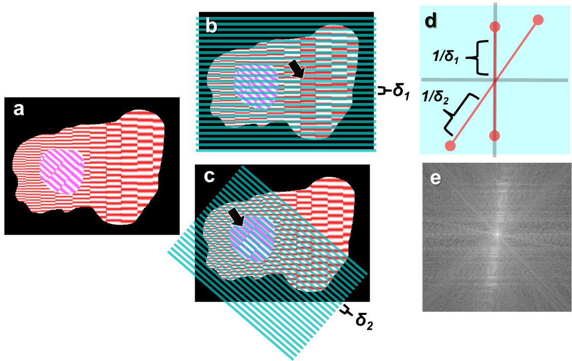
Schematic drawing of how spatial frequency components are extracted using a two-dimensional Fast Fourier Transform (2D-FFT). This provides information about grating lines, equally spaced lines with a pitch ( ${𝛅}_1$ .or ${𝛅}_2$ in b or c), contained in the original image (a). When we find out a situation where a set of grating lines can be well superimposed (black arrows in b or c), we mark two dots on a map in the right panel (d) at a distance of ${1/𝛅}_1$ or ${1/𝛅}_2$ from the center of the map. This distance is called the spatial frequency, which is an index of the number of grating lines per unit length. This process for all the possible spatial frequencies included in the original image (a) corresponds to a 2D-FFT calculation, and ultimately produces the spatial frequency map shown in e.

2. MATHEMATICAL BACKGROUND OF FFT

Fourier transform is based on the following rules for the calculation of integrals.

  

$${\int }_{-\pi }^{\pi }sin\left(ax\right)dx={[-\frac{1}{a}cos\left(ax\right)]}_{x=-\pi }^{x=\pi }\left(2\right)$$

  

$${\int }_{-\pi }^{\pi }cos\left(ax\right)dx={\left[\frac{1}{a}sin\left(ax\right)\right]}_{x=-\pi }^{x=\pi }\left(3\right).$$

These formulas correspond to the summation process of wave signals such as grating lines in sample images or visible light propagating in a specific space and direction. If you remember the addition or subtraction rules for sine and cosine functions as shown in the following equations,

  

$$sin(a\pm b)x=sin\left(ax\right)\cdot cos\left(bx\right)\pm cos\left(ax\right)\cdot sin\left(bx\right),\left(4\right)$$

  

$$cos(a\pm b)x=cos\left(ax\right)\cdot cos\left(bx\right)\mp sin\left(ax\right)\cdot sin\left(bx\right),\left(5\right)$$

you can derive the following integration. Please, ask AI teachers of mathematics to find out how to derive these addition or subtraction rules. By modifying these equations, (4) and (5), we will obtain the equation (see Appendix 2 for details),

  

$$sin\left(ax\right)sin\left(bx\right)=\frac{1}{2}\{cos(a-b)x-cos(a+b)x\}.\left(6\right)$$

The following discussion is restricted to the cases with $a$ and $b$ of integers. These integers correspond to the number of grating lines per unit length of $2\pi$ . The following integration formula (7) corresponds to the summation of equation (6) over the range from $x=-\pi$ to $x=\pi$ .

  

$${\int }_{-\pi }^{\pi }sin\left(ax\right)sin\left(bx\right)dx=\frac{1}{2}{\int }_{-\pi }^{\pi }\{cos(a-b)x-cos(a+b)x\}dx$$

  

$$={\frac{1}{2}[\frac{1}{a-b}sin(a-b)x-\frac{1}{a+b}sin(a+b)x]}_{x=-\pi }^{x=\pi }=0,\left(7\right)$$

since $sin(a\pm b)\pi =0$ for any combination of $a$ and $b$ of integers. However, this calculation is correct only when $a\ne b$ . If the denominator $a-b$ is 0, equation (7) cannot be calculated.

In this case, $a=b$ , we need to calculate differently as follows.

  

$${\int }_{-\pi }^{\pi }sin\left(ax\right)sin\left(bx\right)dx=\frac{1}{2}{\int }_{-\pi }^{\pi }\{cos(a-b)x-cos(a+b)x\}dx=\frac{1}{2}{\int }_{-\pi }^{\pi }\{1-cos(a+b)x\}dx$$

  

$$={\frac{1}{2}[x-\frac{1}{a+b}sin(a+b)x]}_{x=-\pi }^{x=\pi }=\pi .\left(8\right)$$

This unique property of the integrals in (7) and (8) is simple, $0$ or $\pi$ , but it is the most crucial point in understanding the mathematical principles of the Fourier transform as well as diffraction optics. That is, the integral value of

  

$${\int }_{-\pi }^{\pi }sin\left(ax\right)sin\left(bx\right)dx\left(9\right)$$

is $\pi$ only when $a=b$ , otherwise = 0. It shouldn’t be too difficult to derive to the following rules in a similar way of calculation, the integral value of

  

$${\int }_{-\pi }^{\pi }cos\left(ax\right)cos\left(bx\right)dx\left(10\right)$$

is $\pi$ only when $a=b$ , otherwise = 0 (Appendix 2). Furthermore,

  

$${\int }_{-\pi }^{\pi }sin\left(ax\right)cos\left(bx\right)dx$$

and

  

$${\int }_{-\pi }^{\pi }cos\left(ax\right)sin\left(bx\right)dx\left(11\right)$$

are always = 0 for any combination of $a$ and $b$ . These equations are easy to understand if you know the basic rules of analytical mathematics, such as calculus. Using the above steps, we can derive the following new rules.

  

$$\frac{1}{\pi }{\int }_{-\pi }^{\pi }f\left(x\right)cos\left(kx\right)dx=A_k,\left(12\right)$$

  

$$\frac{1}{\pi }{\int }_{-\pi }^{\pi }f\left(x\right)sin\left(kx\right)dx=B_k,\left(13\right)$$

where

  

$$f\left(x\right)=\sum _{j=0}^{j=N}{A}_{j}cos\left(jx\right)+B_{j}sin\left(jx\right).\left(14\right)$$

That is, if $f\left(x\right)$ can be written as a sum of cosine and sine waves of various frequency of $j$ ( $j$ =0 to $N$ ), where $2\pi /j$ is the wavelength, or $j/2\pi$ is the wave frequency, we can extract of $A_k$ and $B_k$ using the equation (12) and (13). The process of extracting a series of wave amplitudes of $A_k$ and $B_k$ from the original function of $f\left(x\right)$ corresponds to the process of Fourier transform. This rule is approximately true, because almost all real wave patterns or signal functions described by $f\left(x\right)$ can be assumed as the sum of waves with a series of amplitude values, $A_j$ and $B_j$ of frequency $j/2\pi$ .

Similar mathematical techniques can also be applied to two-dimensional signals (Figure 2). For example, in one of the 2D-FFT processes shown in Figure 1b, please imagine the situation where the original two-dimensional image is projected onto an arbitrary side axis to obtain the function $f\left(x\right)$ representing the profile of image brightness. We then execute FFT calculations using the formula (12)―(14). Thus, for $f\left(x\right)$ , we obtain amplitudes $A_k$ and $B_k$ of $cos\left(kx\right)$ and $sin\left(kx\right)$ , $k=2\pi /\delta$ , respectively.

Figure 2

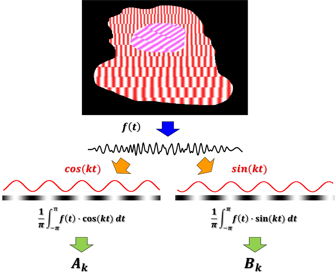
How we can extract the spatial frequency components in an observing 2D-image. First, we create a density map corresponding to a 1D projection from the original image (blue arrow), which can be described by a profile function, here f(x). Next, we calculate functions f(x)∙cos(kx) and f(x)∙sin(kx). Following the mathematical rules explained in the text, we can integrate and extract the amplitudes of A_k for cos(kx) or B_k for sin(kx). This process corresponds to the schematic diagrams explained in Figure 1a and 1d.

To be more mathematically precise, $A_k$ and $B_k$ are independent quantities. It is not possible to infer $B_k$ of $sin\left(kx\right)$ from $A_k$ of $cos\left(kx\right)$ , and vice versa. In other words, both $A_j$ and $B_j$ are necessary to describe correct $f\left(x\right)$ . The ratio values of $A_j$ to $B_j$ is called the phase information for the frequency $j$ ( $j$ =0 to $N$ ) and is necessary to describe the original $f\left(x\right)$ . The phase information is also quite important for light microscopes. We can reconstruct images by optical lenses when both $A_{k}sin\left(kx\right)$ and $B_{k}cos\left(kx\right)$ are collected and projected onto the imaging plane. In the case of the image shown in Figure 2, both $A_{k}sin\left(kx\right)$ and $B_{k}cos\left(kx\right)$ , i.e., the phase information are essential for the accurate reproduction of the image recovering by an optical lense. Problems usually happens when we cannot use lenses for a special type of electromagnetic wave, e.g., X-ray. In this article, this mathematically precise discussion of phase information will be omitted for simplicity. It’s unnecessary for understanding Abbe theory and microscope resolution.

3. DIFFRACTION OF LIGHT FROM GRIDS

Diffraction is a phenomenon that we can see in all kinds of propagating waves. For example, waves traveling on water surfaces can pass through obstacles, and go round boats and small islands. Similarly, light rays travel in a straight line if there are no obstacles, but when they hit an obstacle, they bend as if reborn at the interfered point. This phenomenon is called optical diffraction. Due to the diffraction of light by specimen under microscope, we can detect and observe materials.

Diffracted light waves from the sample are dispersing randomly at various angles, but they can be detected in the case when diffracted waves are superimposed and accumulated in a specific region in space. This phenomenon of superimposition is called optical interference, because waves with the same wavelength and vibration phase can be summed up and intensified by each other. Longer, more continuous waves with the same phase and wavelength can be added or canceled each other anywhere and anytime easier comparing to shorter and more random waves. This property, long and short, or regular and irregular nature of propagating light waves is called coherency. How light coherency affects the image quality and resolution will be discussed at the end of this article.

An ideal situation where a parallel light wave, $A\cdot sin\omega t$ , passing through a set of grating lines with a spacing of $\delta$ is shown in Figure 3. If the light waves diffracted from the grating lines travel parallel to the incident beam, at a paraxial angle of zero, they will interfere with each other and overlap synchronously to produce a strong signal. This beam is called the zeroth (0^th) order diffraction (Figure 3a). In addition, similar situations can occur for diffracted light at a specific angle of + $\theta$ (Figure 3b, 3c). In these cases, the phase of the diffracted light from each grating is shifted by a length exactly to one wavelength. These are called the +1^st and -1^st-order diffraction for + $\theta$ and $-\theta$ of diffracted angle, respectively. As shown in the inset depicting right-angle triangles, there is a fixed relation between $\delta$ and $\theta$ as expressed by the equation,

  

$$\delta =\frac{\lambda }{sin\theta },\left(15\right)$$

  

$$\delta =\frac{\lambda }{n\cdot sin\theta }.\left(16\right)$$

Incident beam parallel to the optical axis generates all three diffraction beams of 0^th and +1^st order when we observe through regular grating lines with a spacing of $\delta$ , the density map of which can be described by

$sin\left(\frac{2\pi }{\delta }x\right)\left(17\right).$

From the mathematical description in the previous section, we can easily predict what would happen if a specimen represented by a certain density profile of $f\left(x\right)$ is overlapped with this grating line as in Figure 3d. It gives us the superimposed signals of

  

$$f\left(x\right)\cdot sin\left(\frac{2\pi }{\delta }x\right).\left(18\right)$$

After integration as shown in Figure 2, we can extract the amplitude information of $B_k$ . Similarly, $A_k$ can be calculated by using another cosine filtering of

  

$$f\left(x\right)\cdot cos\left(\frac{2\pi }{\delta }x\right).\left(19\right)$$

This is the very mechanism of Fourier transform that can extract $A_k$ and $B_k$ using light beam and grating lines. In this case using a single set of grating lines with a specific spatial frequency $2\pi /\delta$ , we can successfully extract a signal of spatial frequency $2\pi /\delta$ from $f\left(x\right)$ as the +1^st order diffraction beam at a specific paraxial angle $\theta$ as estimated by equations (16) (Figure 3d and Figure 4a).

Figure 3

Diagrams showing the grating pattern under a microscope and the diffraction light from the specimen. Here, the grating lines are shown as a black-and-white pattern of cross-sections. Grating lines are shown here as black and white patterns. Regular grating lines (a―c), and grating lines plus sample (d) are illuminated by a collimated beam with a synchronous phase of waves. a, a beam penetrates the sample and propagates parallel to the incident beam direction. The light passing through the grating pattern can be synchronously summed, which is called zeroth (0^th) order diffraction. b and c, Diffracted lights can be also synchronously summed with a difference of plus or minus one wavelength ( $\pm 𝛌$ ) respectively, which are called +1^st and -1^st-diffraction orders. d, same situation as b, but the sample with the pattern of density profile $𝐟\left(𝐱\right)$ is also superimposed on the regular grating lines. A summed-up signal of $𝐟\left(𝐱\right)\cdot 𝐬𝐢𝐧\left(2𝛑/𝐝\times 𝐱\right)$ is observed as the 1^st-order diffraction instead of $sin\left(2𝛑/𝐝\times 𝐱\right)$ similarly as in the case of Figure 1b/c. The angle $𝛉$ can be defined by the inserted equation: where $𝐝$ is the spacing of gratings.

Figure 4

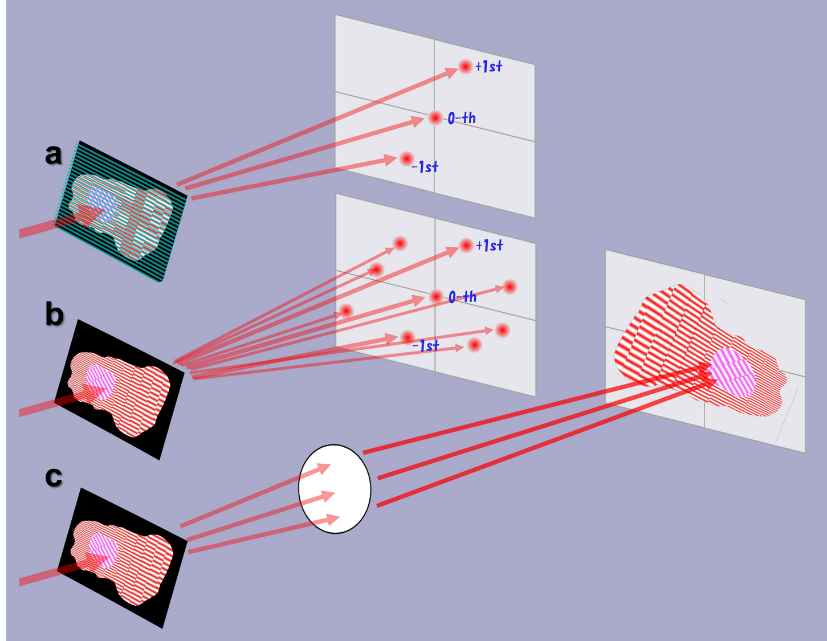
Diagrams showing how the illumination beam light diffracts, creating a magnified image of the specimen. a, as shown in Figure 1b and 1c, where the specimen is observed with overlapping grating lines with a fixed spacing of $\delta$ , three beams corresponding to 0^th and +1^st-order diffraction are observed. Diffracted lights are observed as +1^st-order diffraction spots on a screen placed on the right side. b, a diffraction pattern that can be simulated by 2D-FFT will be observed when we remove the grating line in a since the observing specimen should contain various signals with different tilt angles and spatial frequencies. c, illustrating what will happen when we make a magnified image through a lens. Due to the physical limitations of the lens diameter, it is not possible to collect all the diffracted beams, and ultimately only para-axial light (beams at low angles from beam axis) is collected. According to the diffraction laws as shown in Figure 2b and 2c, the diffracted beams corresponding to lower spatial frequencies are collected through an optical lens.

Here, I would like to revisit the discussion of the phase information after the Fourier transform, or the beam diffraction from the specimen. The observed light intensity of +1^st-order diffraction is equal to the value of ${A_k}^2{{+B}_k}^2$ . However, we cannot know $A_k$ or $B_k$ separately, which are necessary for us to obtain the shape of original function $f\left(x\right)$ . This means that we cannot recover the original image data from the intensity data of light diffraction alone. It is a problem that must be solved when we cannot use lenses to reconstruct original images as in X-ray crystallography. In X-ray crystallography, original molecular shapes cannot be easily inferred from the diffraction intensities of X-ray beam alone. In the case of optical microscopes, we are happy to be able to use optical lens system to collect the diffracted beams together and reconstruct original information of the specimen image. However, as we will see below, it is not possible to collect all angles of the diffracted beam, and this limits the capabilities of optical microscope, as Abbe made clear.

Imagine a situation where we remove the filter of the grating lines of $2\pi /\delta$ frequency and collect signals of all diffraction angles together (Figure 4b). The light beam now works like a Fourier transformer, revealing numerous angles of +1^st order diffraction signals corresponding to various spatial frequency components included in the original specimen, as shown in Figure 4b. This information corresponds to the 2D-FFT of the intensity mapping of ${A_k}^2{{+B}_k}^2$ as shown in Figure 1d and 1e.

The size of each diffraction spots appearing in the screen placed on the right side is same to that of the original incident beam (Figure 4). To obtain a magnified image, we must place a lens after the specimen that focuses the diffracted light into small spots as shown in Figure 4c. As this schematic drawing indicates, by obtaining magnified images through a lens, we must choose the light beams of paraxial diffraction within a restricted paraxial angles less than the lens diameter. If the maximal angle of diffraction beam that can enter the lens is ${\theta }_0$ from the optical axis, the minimum spacing $d_0$ of grating lines we can observe is estimated by the equation,

  

$$d_0=\frac{\lambda }{n\cdot sin{\theta }_0}.\left(20\right)$$

This is the resolution limit of optical microscope defined by Abbe. By using a lens with a larger diameter, light with diffraction angles larger than ${\theta }_0$ can be collected, and grating lines smaller than $d_0$ of spacing can be observed. In other words, to obtain higher resolution, it is essential to increase the value of $n\cdot sin{\theta }_0$ (numerical aperture), which is exactly what Abbe emphasized.

Optical lenses work as a filter to choose lower diffraction angles than ${\theta }_0$ , or gratings of lower spatial frequency from original specimen images than ${1/d}_0$ . We can call this property of optical lens as low pass filter, LPF. LPF properties can be simulated by an image processing tool like Image-J software. We need only to restrict center area of calculated 2D-FFT, just mimicking data selection by optical lens and recontract the magnified image by reversed calculation of FFT (Figure 5, Movie S1, S2).

Figure 5

Diagrams showing how diffraction and lens filtering modify the observed images. As shown in Figure 4, lens works as a filter to collect the diffraction beams of lower spatial frequencies. We can call it the effect of low-pass filter (LPF). The illumination light and beam diffraction works as a 2D-FFT converter, which can be mimicked by conventional image processing tools like Image-J. We can also mimic the lens function by selecting the center area for the calculation for reverse FFT (rFFT). a, example when observing the model specimen shown in Figure 1b (Movie S1). When observing a small point as a specimen, circular rings corresponding to the Airy disk pattern or point spread function (PSF) is observed (Movie S2).

When a small point of material is placed under an optical microscope as a sample, a LPF image is obtained as shown in Fig. 5b. The magnified image consists of many concentric circles, which is called Airy disk pattern, or in a more modern way, point-spread function (PSF). The radius of the smallest circle in the Airy disc pattern corresponds to the size of resolution limit since we cannot distinguish two points if they are placed nearer than the disc radius. The mathematical expression corresponding to the shape of PSF is useful for describing the functional properties of lens or the entire microscope system and is used for numerical calculation to correct and adjust blurred fluorescent images using a technique called “deconvolution”. An optical microscope system can be viewed as a set of image transformers, including 2D- FFTs and LPFs, and these processes can be mathematically described as convolution. “Deconvolution” refers to a mathematical inverse operation that restores an image of sample through numerical estimations using a PSF.

4. SUPER RESOLUTION

Abbe’s assumption is perfect and we cannot resolve grating line spaces narrower than that defined by the equation (20). In actual microscope systems, the light rays shown in Figure 3 are not true, where we use parallel and synchronous light waves with high coherency. There are two issues to be explained here. First, such parallel illumination conditions do not hold when using conventional light sources as halogen lamps with tungsten filament or LED illuminators having a certain area of luminescent material. The emitted light beams are not synchronized and do not have the same wavelength. Therefore, the light rays illuminating the specimens cannot be perfectly parallel to the axis of optical system. Another problem is that highly coherent light cannot produce a magnified image. More precisely, highly coherent light (e.g., laser beam light) diffracted from observing specimens tends to constantly interfere with itself throughout the microscope, forming a highly noisy pattern in the magnified image called “speckle noise”. We cannot avoid this noisy situation unless beam path is carefully confined inside the microscope, as in a confocal microscope system (White et al., 1987).

Hopkins demonstrated the resolution limit in the case of more practical conventional microscopes (Hopkins and Barham, 1950). Through his discussion using Fourier optics, he proposed equation (1) shown in section 1. His parameter of $K$ ranges from 0.5 to 1, which varies depending on how the coherent and parallel light we are using. Using an enlarged small point sample shown in Figure 5b and inverse FFT calculations, we can further simulate the situation when observing two points under incoherent illumination (Figure 6, Movie S3). Two-point images (PSFs) can be distinguished on the enlarged image if they are separated by more than 0.61 $\times$ Airy disk radius. Thus,

$d_0=0.61\times \frac{\lambda }{n\cdot sin{\theta }_0}.\left(21\right)$

is the resolution limit under a conventional illumination. This is also the limit to which the exact distance between two points can be determined.

Figure 6

Diagram showing simulation results of two small dots are observed under a microscope. The numbers represent the distance between the two dots as relative values of the Airy disc radius ( $r$ ). The closer the dots are, the more the observed images merge and the more difficult to be resolved. Around with the relative distance of $r=0.61$ is the resolution limit under this condition. Separation is possible if the dots are different colors and observed at different times (Movie S3).

So how can we achieve a super-resolution less than $d_0$ , better than the equation (1) and (21)? Abbe’s proposal is to use an optical system called oblique illumination to the light source angle, allowing two diffraction beams, the 0^th and +1^st order diffraction beams (excluding the -1^st order diffracted beam), to be introduced into objective lens. This improves $d_0$ by approximately half. Further improvement of the resolution beyond the Abbe limit is impossible without using a confocal fluorescence microscope. New additional techniques for confocal fluorescence microscopy allowed us the fine tuning of the illumination of fluorophores. For example, STED method can reduce the size of PSF by focusing two independent laser beams of different wavelengths (Hell and Wichmann, 1994), while SIM employs a technique that superimposes an artificial, regular grid pattern of illumination onto the sample (Gustafsson, 2000). Furthermore, STORM allows us to distinguish two points closer than $d_0$ by making them appear at different times (Rust et al., 2006), which is called a “time-resolved” condition rather than a “spatially-resolved” condition of our conventional microscopes (Movie S3). The resolution limit under the time-resolved conditions depends on the accuracy we can determine the center of PSF separately appearing on a magnified image. This accuracy is not determined by Abbe limit but purely by the signal intensity, i.e., the temporal and areal integration of image brightness, which has been shown practically as small as a scale of nano-meters or pico-meters (Kamimura, 1987; Noda and Kamimura, 2008; Ram et al., 2006, von Diezmann et al., 2017).

5. PERSPECTIVES

How can we overcome the Abbe limit? This has been considered theoretically impossible because there were no doubts about his theory. The milestone toward overcoming the Abbe limit was the revolutionary development of now widely used confocal fluorescence microscope. Of course, that alone is not enough to truly break through the limit of resolution. Discovery of stable and easy-to-use fluorescent dyes, as well as breakthroughs in computer-aided optics and laser techniques, have driven the revolution in super resolution microscopy. This article is written for young students who may not be true developers of new optical systems, but who will be powerful users of optical microscopy in the future. I believe that understanding the precise mechanisms behind the limitations of optical system will help us approach the true limits of biological science and bring about new major innovations.

ACKNOWLEDGEMENT

This article is based on lectures given by the author at the University of Tokyo as well as at Chuo University in Tokyo, Japan from 2000 to 2025. Students of basic biology are often faced with enormous efforts to understand the complex and diverse world of organisms that have evolved over billions of years in our ecosystems. For them, the theoretical world of physics and mathematics seems entirely different and challenging. This article was prepared for them by providing many illustrations that would help them understand optics firsthand and open new doors in science. I would like to thank them for their efforts in trying to understand my lectures over the years.

MOVIES

Movie S1. Simulation of low-pass filtering of microscope

https://zenodo.org/records/21276226/preview/MovieS1.mp4

Simulation of the low-pass filter (LPF) characteristics of a microscope lens when observing the specimens shown in Figures 1 and 2 placed under a microscope. After selecting diffraction signals at various angles, i.e., different diameters of the central region of the 2D-FFT, the low-pass filter effect is simulated by inversing FFT.

Movie S2. Simulation of low-pass filtering of microscope

https://zenodo.org/records/21276226/preview/MovieS2.mp4

Simulation of the low-pass filter (LPF) characteristics of a microscope lens when observing a single point as a specimen under a microscope. After selecting diffraction signals at various angles, i.e., different diameters of the central region of the 2D-FFT, the low-pass filter effect is simulated by inversing FFT.

Movie S3. Simulation to show how a two-spot specimen appears under a microscope

https://zenodo.org/records/21276226/preview/MovieS3.mp4

Two small dots at different distances are shown in a magnified image after passing through a low-pass filter. When the dots are placed closer than the resolution limit, the two dots cannot be distinguished. However, the situation should change when we can observe them appearing in different colors with alternative timing. By measuring the center of spots appearing separately, this time-resolved method enabled us the observation with super-resolution.

REFERENCES

•  Abbe,  E. (1873) Beitrage zur Theorie des Mikroskops und der mikroskopischen Wahrnehmung. Archiv fur mikroskopische Anatomie Archiv fur mikroskopische Anatomie Entwichlungsmech 9: 413–468.
•  Abbe,  E. and  Fripp,  H. (1874) A contribution to the theory of the microscope, and the nature of microscopic vision. Proceedings of the Bristol Naturalists' Society, New Series 1: 200–258.
•  Cooley , J.W. and  Tukey , J.W. (1965) An algorithm for the machine calculation of complex Fourier series. Mathematics of computation 19: 297–301.
• Goodman, J.W. (2017) Introduction for Fourier optics. WH. Freeman, New York.
•  Gustafsson,  M. (2000) Surpassing the lateral resolution limit by a factor of two using structured illumination microscopy. Journal of microscopy 198: 82–87.
•  Hecht,  E. (2015) Optics. Pearson, Boston.
•  Hell , S.W. and  Wichmann,  J. (1994) Breaking the diffraction resolution limit by stimulated emission: stimulated emission depletion microscopy. Optics letters 19: 780–782.
•  Hopkins , H. H. and  Barham , P. M. (1950) The influence of the condenser on microscopic resolution. Proceedings of the Physical Society 63: 737–744.
• Inoué, S. and Spring, K.R. (1997) Video Microscopy: The fundamentals. Plenum Press, New York.
•  Kamimura,  S. (1987) Direct measurement of nanometric displacement under an optical microscope. Applied optics 26: 3425–3427.
•  Noda,  N. and  Kamimura,  S. (2008) A new microscope optics for laser dark-field illumination applied to high precision two-dimensional measurement of specimen displacement. Review of Scientific Instruments 79: 023704.
•  Ram  S.,  Ward , E.S. and  Ober,  R. (2006) Beyond Rayleigh’s criterion: A resolution measure with application to single-molecule microscopy. Proceedings of the National Academy of Sciences 103: 4457–4462.
•  Rayleigh,  L. (1879) Investigations in optics, with special reference to the spectroscope. Philosophical Magazine and Journal of Science 8: 261–274.
•  Rust   M.J.,  Bates M. and  Zhuang,  X. (2006) Stochastic optical reconstruction microscopy (STORM) provides sub-diffraction-limit image resolution. Nature Methods 3: 793–795.
• Slayter, E.M. and Slayter, H.S. (1993) Light and electron microscopy. Cambridge University Press, Cambridge.
•  Sparrow , C. M. (1916) On spectroscopic resolving power. Astrophysical Journal 44: 76–86.
•  von Diezmann,  L.,  Schechtman,  Y. and  Moemer , W.E. (2017) Three-dimensional localization of single molecules for super-resolution imaging and single-particle tracking. Chemical Reviews 117: 7244–7275.
•  White , J. G.,  Amos , W. B. and  Fordham,  M. (1987) An evaluation of confocal versus conventional imaging of biological structures by fluorescence light microscopy. Journal of Cell Biology 105: 41–48.

APPENDIXES

Appendix 1

List of symbols and technical terms used in the text

$d$ or $d_0$	resolution limit
$\delta$	regular spacing of grating lines
$1/\delta$	spatial frequency, number of grating lines in a unit length
$\lambda$	wavelength of light
LPF	low pass filter
$n\cdot \sin \theta$	numerical aperture
$n$	refractory index
PSF	point-spread function
STED	Stimulated Emission Depletion
SIM	Structured Illumination Microscopy
STORM	Stochastic Optical Reconstruction Microscopy
$\theta$	incident angle of light beam for objective lens
${\theta }_0$	incident angle limit for objective lens that define resolution

Appendix 2

Mathematical process will be described here to derive the equation (6) from the addition or subtraction rules in equations (4) and (5) of the main text or in the following equations,

  

$$sin(a+b)x=sin\left(ax\right)\cdot cos\left(bx\right)+cos\left(ax\right)\cdot sin\left(bx\right),\left(4a\right)$$

  

$$sin(a-b)x=sin\left(ax\right)\cdot cos\left(bx\right)-cos\left(ax\right)\cdot sin\left(bx\right),\left(4b\right)$$

  

$$cos(a+b)x=cos\left(ax\right)\cdot cos\left(bx\right)-sin\left(ax\right)\cdot sin\left(bx\right),\left(5a\right)$$

  

$$cos(a-b)x=cos\left(ax\right)\cdot cos\left(bx\right)+sin\left(ax\right)\cdot sin\left(bx\right).\left(5b\right)$$

By summing two equations $\left(4a\right)plus\left(4b\right)$ as well as $\left(5a\right)plus\left(5b\right)$ , we can get

  

$$sin(a+b)x+sin(a-b)x=2sin\left(ax\right)\cdot cos\left(bx\right),\left(4c\right)$$

  

$$cos(a+b)x+cos(a-b)x=2cos\left(ax\right)\cdot cos\left(bx\right).\left(5c\right)$$

Similarly, by calculating $\left(4a\right)minus\left(4b\right)$ as well as $\left(5a\right)minus\left(5b\right)$ , we can get

  

$$sin(a+b)x-sin(a-b)x=2cos\left(ax\right)\cdot sin\left(bx\right),\left(4d\right)$$

  

$$cos(a+b)x-cos(a-b)x=-2sin\left(ax\right)\cdot sin\left(bx\right).\left(5d\right)$$

If you flip the right and left sides the equation $\left(4c\right)$ and executing its integration,

  

$$sin\left(ax\right)cos\left(bx\right)=\frac{1}{2}[sin(a+b)x+sin(a-b)x],$$

  

$${\int }_{-\pi }^{\pi }sin\left(ax\right)\cdot cos\left(bx\right)dx=\frac{1}{2}{\int }_{-\pi }^{\pi }\{sin(a+b)x+sin(a-b)x\}dx,\left(4c\prime \right)$$

are given. Similarly, from $4d$ , 5c and 5d we can derive the following equations,

  

$${\int }_{-\pi }^{\pi }cos\left(ax\right)\cdot sin\left(bx\right)dx=\frac{1}{2}{\int }_{-\pi }^{\pi }\{sin(a+b)x-sin(a-b)x\}dx,\left(4d\prime \right)$$

  

$${\int }_{-\pi }^{\pi }cos\left(ax\right)\cdot cos\left(bx\right)dx=\frac{1}{2}{\int }_{-\pi }^{\pi }\{cos(a+b)x+cos(a-b)x\}dx,\left(5c\prime \right)$$

  

$${\int }_{-\pi }^{\pi }sin\left(ax\right)\cdot sin\left(bx\right)dx=-\frac{1}{2}{\int }_{-\pi }^{\pi }\{cos(a+b)x-cos(a-b)x\}dx,\left(5d\prime \right)$$

respectively. The results of these integrations are quite different depending on the situations whether $a\ne b$ or $a=b$ . Please, remember this is the most crucial point when you are going to understand the principle of FFT.

If $a\ne b$ , the result of integration $\left(4c\prime \right)$ ,

  

$${\int }_{-\pi }^{\pi }sin\left(ax\right)\cdot cos\left(bx\right)dx=\frac{1}{2}{\int }_{-\pi }^{\pi }\{sin(a+b)x+sin(a-b)x\}dx$$

  

$$={\frac{1}{2}[\frac{1}{a+b}cos(a+b)x-\frac{1}{a-b}cos(a-b)x]}_{x=-\pi }^{x=\pi }$$

  

$$={\frac{1}{2}[\frac{cos(a+b)\pi -cos\{-(a+b)\pi \}}{a+b}-\frac{cos(a-b)\pi -cos\{-(a-b)\pi \}}{a-b}]}_{}^{}\left(4c^{″}\right)$$

is always zero because $cos\left(z\right)-cos(-z)$ is always zero for any value of z.

Similarly, the result of integration $\left(4d\prime \right)$ ,

  

$${\int }_{-\pi }^{\pi }cos\left(ax\right)\cdot \cdot sin\left(bx\right)dx=\frac{1}{2}{\int }_{-\pi }^{\pi }\{sin(a+b)x-sin(a-b)x\}dx$$

  

$$={\frac{1}{2}[\frac{1}{a+b}cos(a+b)x+\frac{1}{a-b}cos(a-b)x]}_{x=-\pi }^{x=\pi }$$

  

$$={\frac{1}{2}[\frac{cos(a+b)\pi -cos\{-(a+b)\pi \}}{a+b}+\frac{cos(a-b)\pi -cos\{-(a-b)\pi \}}{a-b}]}_{}^{}\left(4d^{″}\right)$$

is always zero.

In the case of integration in $\left(5c\prime \right)$ , the way of calculation is a bit different, but

  

$${\int }_{-\pi }^{\pi }cos\left(ax\right)\cdot cos\left(bx\right)dx=\frac{1}{2}{\int }_{-\pi }^{\pi }\{cos(a+b)x+cos(a-b)x\}dx$$

  

$$={\frac{1}{2}[\frac{1}{a+b}sin(a+b)x+\frac{1}{a-b}sin(a-b)x]}_{x=-\pi }^{x=\pi }$$

  

$$={\frac{1}{2}[\frac{sin(a+b)\pi -sin\{-(a+b)\pi \}}{a+b}+\frac{sin(a-b)\pi -sin\{-(a-b)\pi \}}{a-b}]}_{}^{}\left(5c^{″}\right)$$

is always zero because $sin\left(m\pi \right)$ is always zero for any integer of $m$ .

Similarly, in the case of integration in $\left(5d\prime \right)$ ,

  

$${\int }_{-\pi }^{\pi }sin\left(ax\right)\cdot sin\left(bx\right)dx=-\frac{1}{2}{\int }_{-\pi }^{\pi }\{cos(a+b)x-cos(a-b)x\}dx$$

  

$$=-{\frac{1}{2}[\frac{1}{a+b}sin(a+b)x-\frac{1}{a-b}sin(a-b)x]}_{x=-\pi }^{x=\pi }$$

  

$$={\frac{1}{2}[\frac{sin(a+b)\pi -sin\{-(a+b)\pi \}}{a+b}-\frac{sin(a-b)\pi -sin\{-(a-b)\pi \}}{a-b}]}_{}^{}\left(5d″\right)$$

is always zero. In summary, all the formulas of integration from $\left(4c\prime \right)$ to $\left(5d\prime \right)$ are zero in case $a\ne b$ as indicated by the equations (10) and (11) in the main text.

When $a=b$ , the calculating way of integration is quite different.

  

$${\int }_{-\pi }^{\pi }sin\left(ax\right)\cdot cos\left(bx\right)dx=\frac{1}{2}{\int }_{-\pi }^{\pi }\{sin(a+b)x+sin(a-b)x\}dx$$

  

$$=\frac{1}{2}{\int }_{-\pi }^{\pi }sin(a+b)xdx=-{\frac{1}{2}[\frac{1}{a+b}cos(a+b)x]}_{x=-\pi }^{x=\pi }=0\left(4c^{‴}\right).$$

  

$${\int }_{-\pi }^{\pi }cos\left(ax\right)\cdot sin\left(bx\right)dx=\frac{1}{2}{\int }_{-\pi }^{\pi }\{sin(a+b)x-sin(a-b)x\}dx$$

  

$$=\frac{1}{2}{\int }_{-\pi }^{\pi }sin(a+b)xdx=-{\frac{1}{2}[\frac{1}{a+b}cos(a+b)x]}_{x=-\pi }^{x=\pi }=0\left(4d^{‴}\right).$$

However,

  

$${\int }_{-\pi }^{\pi }cos\left(ax\right)\cdot cos\left(bx\right)dx=\frac{1}{2}{\int }_{-\pi }^{\pi }\{cos(a+b)x+cos(a-b)x\}dx$$

  

$$=\frac{1}{2}{\int }_{-\pi }^{\pi }\{cos(a+b)x+1\}dx={\frac{1}{2}[\frac{1}{a+b}sin(a+b)x+x]}_{x=-\pi }^{x=\pi }=\pi \left(5c″\right)$$

  

$${\int }_{-\pi }^{\pi }sin\left(ax\right)\cdot sin\left(bx\right)dx=-\frac{1}{2}{\int }_{-\pi }^{\pi }\{cos(a+b)x-cos(a-b)x\}dx$$

  

$$=-\frac{1}{2}{\int }_{-\pi }^{\pi }\{cos(a+b)x-1\}dx=-{\frac{1}{2}[\frac{1}{a+b}sin(a+b)x-x]}_{x=-\pi }^{x=\pi }=\pi .\left(5d″\right)$$

Both results are $\pi$ as shown by the equations (8) and (10) in the main text. Examples of integration formulars explained here corresponds to the schematic drawings in Figure 1 and Figure 2, that is, by superimposing $f\left(x\right)$ with $cos\left(kx\right)$ or $sin\left(kx\right)$ , $A_k$ and $B_k$ are efficiently extracted as shown by equations (12―14). A significant point to be stressed here should be the function of light beams diffracted from specimens; light beams work like a Fourier Transformer that extract the information of amplitudes, $A_k$ and $B_k$ of corresponding spatial frequencies, and separate them efficiently by different beam angles as shown in Figure 3 and Figure 4.