Human age estimation from lower-canine pulp volume ratio based on Bayes’ theorem with modern Japanese population as prior distribution

Abstract

Pulp volume decreases throughout life owing to secondary dentin deposition. Here, we present a Bayesian approach for human age estimation on the basis of the pulp volume ratio from lower-canine teeth. We measured the pulp and tooth volumes of 363 subjects (209 males, 154 females) of known age based on three-dimensional imageries from microcomputed tomography scans. Pulp volume ratio was defined as pulp/tooth volume within the root portion (PVRrt) and its reduction with age was modeled by simple statistical assumptions to produce a likelihood function of PVRrt by fitting the model to the observed data. Following Bayes’ theorem, we obtained the probability density function (PDF) of estimated age for a given PVRrt, for males, females, and gender unknowns; we used the modern Japanese population as of 2012 as prior age distribution. The PDF of estimated age provided the mean and 50%, 70%, and 90% prediction intervals, based on which we compared the present age- estimation method with that of Brooks and Suchey (Human Evolution, 5: 227–238), which is based on pubic symphysis metamorphosis. We could not find any advantages of the PVRrt method compared to the Suchey–Brooks method for the case of males or gender unknowns as far as the prediction intervals were concerned. However, for females, the PVRrt method offered comparable precision to the Suchey–Brooks method. Taking into account other advantages such as sustainability of the material and continuous property of the age-indicator value, we conclude that the PVRrt method is useful in forensic cases, especially those involving female victims.

Introduction

Age information is often critical in identifying individual victims in forensic cases. When no written record is available, or when the body is highly decomposed, dentition plays an important role in estimating age. There are several biological age indicators in teeth, including pulp cavity reduction due to secondary dentin deposition. As the secondary dentin grows gradually on the wall of pulp cavity throughout life, the volume of the pulp cavity reduces with age. Today, appositional dentin tissues are distinguished into three types—primary, secondary, and tertiary—based on the time and the causes of formation as well as their histological differences. Primary dentin is formed before tooth maturation and constitutes most of the volume of the tooth. After tooth eruption and root maturation, odontoblasts (dentin-secreting cells) reduce the rate of dentin formation but still physiologically continue to form dentin. This dentin is called secondary dentin. Tertiary dentin is generated as a protective reaction of the dentin–pulp complex against pathological causes such as caries lesion, dentin exposure by attrition and/or inflammation of pulp tissue. When dentin is exposed to oral cavity by caries, attrition, or any other traumas, tertiary dentin develops and fills dentin tubules, preventing bacterial intrusion into the pulp tissue.

The deposition of secondary dentin was first used by Gustafson (1950) for human age estimation in a numerical manner. After scoring the degree of progress in several age-related changes, including secondary dentin deposition, Gustafson regressed the sample age on the scores and obtained an age-estimation formula. To visualize the secondary dentin, the teeth were prepared into ground sections for microscopic observations. While many subsequent studies have worked on ground sections, modifying Gustafson’s method (Dalitz, 1962; Johanson, 1971; Burns and Maples, 1976; Maples, 1978; Maples and Rice, 1979; Kashyap and Koteswara Rao, 1990), Kvaal and Solheim (1994) used radiographs of intact teeth to investigate the degree of secondary dentin development. Since secondary dentin is difficult to distinguish from other types of dentin on a radiograph, Kvaal and Solheim measured the size of the pulp cavity and assessed the degree of shrinkage to represent the secondary dentin development. A radiograph was easier to prepare than ground sections; moreover, radiography could be applied to living humans without extracting the teeth, allowing greater number of samples to be obtained. Therefore, numerous studies have been conducted to date modifying or testing the dental radiograph-based age-estimation methods (Kvaal et al., 1995; Drusini et al., 1997; Kolltveit et al., 1998; Willems et al., 2002; Bosmans et al., 2005; Paewinsky et al., 2005; Cameriere et al., 2007; Meinl et al., 2007; Drusini, 2008; Landa et al., 2009; Du et al., 2011; Cameriere et al., 2013). Meanwhile, with the development of computed tomography (CT) technology, the pulp cavity and the tooth can now be measured in three-dimensional space (Vandevoort et al., 2004; Yang et al., 2006; Someda et al., 2009; Aboshi et al., 2010; Agematsu et al., 2010; Star et al., 2011). In those studies, pulp volume ratios were calculated from the CT images and were used for subsequent regression analyses against a few types of teeth: lower central incisors (Someda et al., 2009; Agematsu et al., 2010), lower first premolars (Aboshi et al., 2010), and lower second premolars (Aboshi et al., 2010; Agematsu et al., 2010). Canines have not yet been studied in large numbers.

Contrary to the significant development of technology to investigate the inside of a tooth, the statistical method for age estimation has not radically changed; analyses based on regression of age on secondary dentin development have been the only methods utilized. In the field of anthropology, Bocquet-Appel and Masset (1982) first pointed out that the age-estimation formulae obtained by such regressions are by no means unique to the biological characters in question but are influenced by the age distributions of the samples used in the analyses, unless the age indicators correlate with age perfectly (e.g. the case in which the correlation coefficient equals 1 or −1). This means that an age-estimation formula is merely population specific, i.e. the underlying age distribution for the target individual should be the same as that of the reference population from which the formula was derived, but the formula cannot be used for individuals possibly with different age distribution. Faced with the fact that there is no universal age-estimation formula independent of the age distribution, we should first determine the age distribution for the target population before attempting to estimate the age of an individual (Hoppa and Vaupel, 2002). In this study, we narrowed the target to modern Japanese, and assumed the age structure of the Japanese population in 2012 published by the Statistics Bureau, Ministry of International Affairs and Communications, Japan (2013) as the age distribution of the target population.

Contrary to regressions of age on age indicators, regressions of age indicators on age could be considered as being independent of the age distribution. In other words, the probability of being at a certain age A conditional on the age indicator being a certain value (or state) I is dependent on the age distribution, but the probability of being I conditional on being A (referred to as likelihood in Bayes’ inference) is basically independent of the age distribution. In this study, we adopted the pulp volume ratio as the age indicator (I) and established a statistical model to describe the likelihood of being I across an age range (A), by fitting a exponential curve to the data sets of observed value and recorded age. With the likelihood and the Japanese population data, we calculated the probability density distribution of estimated age in accordance with Bayes’ theorem. In addition, as the primary objective of this paper, we showed the mean and some prediction intervals on charts so that one can convert a pulp volume ratio of a modern Japanese canine into the probable age range for that individual. Finally, the precision of the estimation was assessed by comparing the prediction intervals with those of the Suchey–Brooks pubic symphysis phase system (Brooks and Suchey, 1990) obtained using a similar Bayesian approach.

When X is a variable which can be measured with no error and Y is a variable which varies depending on X with a certain distribution of error, the regression analysis of X on Y in order to estimate new X (x0) from new Y (y0) is called inverse regression (or inverse calibration). In the case of age estimation, age should be X and age indicator Y as it is more natural to assume that the age indicator varies depending on how long the person has lived (i.e. age) with a certain random variation than to assume the reverse. As mentioned above, inverse regression is not appropriate for age estimation unless the age distribution of the target sample is same as that of the reference sample. Since the critique by Bocquet-Appel and Masset (1982) of the conventional regression approach (inverse regression), the Bayesian approach has been a promising methodology for a new age- estimation scheme (Lucy et al., 1996; Buckberry and Chamberlain, 2002; Gowland and Chamberlain, 2002; Storey, 2007; Kimmerle et al., 2008; Konigsberg et al., 2008; Nagaoka et al., 2008; Prince and Konigsberg, 2008; Prince et al., 2008; Coqueugniot et al., 2010; Langley-Shirley and Jantz, 2010; Thevissen et al., 2010; Nagaoka et al., 2012a, b). The Bayesian approach takes the age distribution of the target population (referred to as prior distribution) into the probability calculation and, therefore, the answer (referred to as posterior distribution) circumvents the above-mentioned problem as it is customized to the target population. As long as the prior distribution and the likelihood are available, the Bayesian approach should be adopted instead of inverse regression analyses for estimating an individual’s age. However, inappropriate prior distribution, of course, will make the posterior distribution deviate from reality. To see how much posterior distributions vary with the choice of prior distribution and how they are compared to a result from the inverse regression, some examples are shown in this paper.

Materials and Methods

Tooth samples

All teeth used in this study were lower canines. Only one side was collected from an individual. The side in the better condition (e.g. less caries, less worn, less post-mortem damage) was chosen when both sides were available. The total number of individuals studied was 363 (209 males and 154 females). The gender and age distribution is shown in Table 1. Out of all samples, 128 teeth were from individual skeletons stored in the University Museum, The University of Tokyo (UMUT), which had been cadavers dating from between 1880s and 1920s. According to the records with the specimens, they were all assumed to be Japanese (sub- sample group K). Another 168 teeth were from collections of individual dentitions stored in UMUT, which had been also cadavers dating from the 1940s–1950s. The names of the medical institutes where the autopsies had been performed were available for 109 out of the 168 specimens. As all the locations were in Japan, we considered the majority of those specimens to be Japanese (sub-sample group F). The remaining 67 teeth were specimens prosthetically extracted from patients who had visited the hospital of the School of Dentistry at Matsudo, Nihon University since the 1970s, and we assumed likewise that majority of the patients were Japanese, despite not having any records about the patients’ ethnicity (sub-sample group M). We used the following sampling criteria:

1. (1) The recorded age should be ≥15 years.
2. (2) The tooth should be sufficiently mature; the volume proportion of pulp canal (excluding branches) in a 5 mm apical root portion should be ≤0.09 (this criterion was made to reduce the large variation in pulp volume ratio around the time of root completion).
3. (3) Lesion (due to caries, post-mortem damage, etc.) should not reach the pulp cavity in the root portion.
4. (4) The tooth should not show a large volume loss (≥1/10 judged by visual appearance) in the root portion.
5. (5) The identification of lower canine should be confirmed It should not be collected if any doubt existed as to its identity. (This is often the case, for example, when there is complete loss of the crown part or morphological abnormality, etc.)
6. (6) Teeth whose ethnicity records are non-Japanese should not be collected.

Table 1 Age and sex distribution of studied samples

Age category (in years)	Male	Female	Total
15–19	18	3	21
20–29	33	29	62
30–39	33	16	49
40–49	32	23	55
50–59	31	22	53
60–69	30	28	58
≥70	32	33	65
Total	209	154	363

CT scan and image processing

To measure volumes of the pulp cavities and the teeth, whole teeth were scanned by microfocal CT (micro-CT). Two micro-CT scanners were used: TXS225-ACTIS (TESCO Corporation, Tokyo, Japan) or SkyScan1173 with NRecon reconstruction software (Bruker-microCT, Kontich, Belgium). The size of element cubes (voxel size) in the reconstructed imagery was equilaterally 0.028 or 0.030 mm, respectively.

Each three-dimensional imagery was further processed using Amira 5.2.2 image-processing software (VSG, Burlington, VT, USA). Before starting tissue segmentation, the voxel size was doubled (i.e. to 0.056 or 0.060 mm) for data-processing efficiency. Then, the images were segmented into ‘air,’ ‘enamel,’ ‘dentin,’ and ‘pulp cavity,’ based on the CT number of each voxel following the half- maximum-height procedure (Spoor et al., 1993). Opening and smoothing processes were used to remove artificial or unnecessary projection on tooth surfaces, although those were not used for the boundary between dentin and pulp cavity. Cementum was included in ‘dentin’ as their CT numbers were too similar to separate. Denticles, the calcified particles that occasionally appear in pulp tissue, were included in ‘pulp cavity.’ Dental calculus was eliminated (i.e. included in ‘air’) by using half-maximum-height or manual segmentation.

Secondly, the longitudinal axis for each tooth was determined as the line which bisects the major part of the root (i.e. the root excluding roughly one-third of the apical tip) into right and left sides equally as viewed from both labiolingual and mesiodistal aspects. A horizontal plane was defined as any flat plane which is perpendicular to the longitudinal axis. After defining the orientation, each segmented tooth imagery was separated into two (coronal and root) portions by the horizontal plane at the height of apical-most point of cementoenamel junction. The coronal portions are prone to external factors that affect the pulp volume ratio, such as tertiary dentin deposition by external stimuli and tooth volume loss by dental wear or caries. To minimize these biases, coronal portions were eliminated from the volume measurement. Thus, only root portions were used for further analyses. However, exceptionally for five specimens in which tertiary dentin occupied the pulp cavity of the above-defined coronal portion completely, the horizontal plane between the coronal and root portions was redefined at the most-coronal point of the ‘pulp cavity’ in order to eliminate the effect of the tertiary dentin (Figure 1).

Figure 1

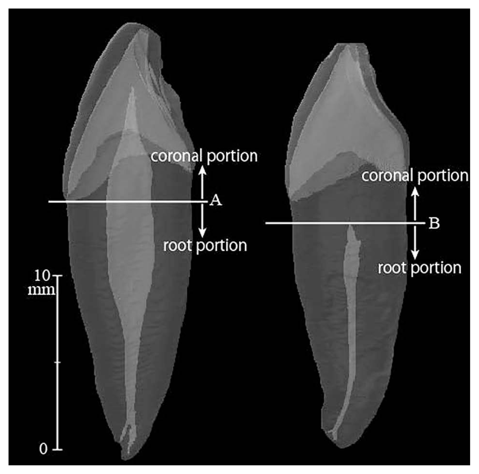
Semi-transparent imageries of lower canine teeth in lateral view. Left: 26 year old female. Right: 53 year old male. The flat horizontal plane that bisects the teeth into coronal and root portions was defined as that at the height of the apical-most point of the cementoenamel junction, or at the height of the coronal-most point of the pulp cavity, whichever was more apical. (A) exemplifies (B) the latter. Only root portions were considered for the analyses in this study.

Third, we measured the volumes of interest by counting the voxels and then calculated the pulp volume ratio in the root portion (hereinafter, PVRrt). The PVRrt is defined as the volume of the pulp cavity divided by the volume of root. The volume of the pulp cavity is the volume of ‘pulp cavity’ within the root portion. The volume of root is the volume of ‘dentin’ within the root portion plus the volume of pulp cavity.

For 24 samples where it was impossible to extract the tooth from the jaw, we scanned it with the jawbone. In this case, segmentation was necessary to remove bone matrices from ‘dentin.’ The CT numbers of bone and dentin were so close that manual segmentation with extra applications of smoothing functions were required.

In another eight cases, in which post-mortem chipping to the root portions had resulted in loss of material, the missing parts were filled in the CT imagery by interpolating between the two unaffected image slices that bound together the affected parts. The resulted gains in the dentin volumes were no more than 5.59% of the root volumes.

Although the definition of the longitudinal axis was a bit vague, the PVRrt value is not radically skewed by an arbitrary choice of the axis. Indeed, when the longitudinal axes of five chosen samples were tilted 10° in random directions, the PVRrt values as defined above did not change more than 2.6%.

Analyses

To confirm that PVRrt reduces with age, samples were divided into seven age categories (15–19, 20–29, 30–39, 40 49, 50 59, 60 69, and ≥70 years), and the mean PVRrt in each category was calculated according to sex. The differences between the neighboring categories were tested by Student’s t-tests. Sex difference was also tested in each age category. Next, differences in PVRrt between teeth with and without lesions such as caries were tested. Although coronal portions were not used for PVRrt calculations, the effect of tertiary dentin was not completely eliminated. While examining all CT imageries, we often found slight tertiary dentin deposition on the pulp wall not only in the coronal portion but also in the root portion. Tertiary dentin is generated at a place on the pulp wall where it is connected to the lesion by dentin tubules. Since dentin tubules run apically from the cementoenamel junction (or root surface) to the pulp, a lesion on the coronal portion can still affect root portion. According to our observations, lesions on the cervical area occasionally caused tertiary dentin in root portions, although those limited to the enamel area rarely did so (Figure 2). To eliminate the effect of sex distribution (females had slightly higher frequencies of cervical lesions and smaller PVRrt than males in the samples), we used only male samples in this test. To equalize the age effects, samples were again divided into those with the 10-year intervals. However, only categories of 40 49, 50 59, 60 69, and ≥70 were eventually tested since the younger categories did not contain enough samples with cervical lesions. After confirming no significant PVRrt differences among the categories 50–59, 60–69, and ≥70, we combined them into one category and tested the difference within the each category by t-tests.

Figure 2

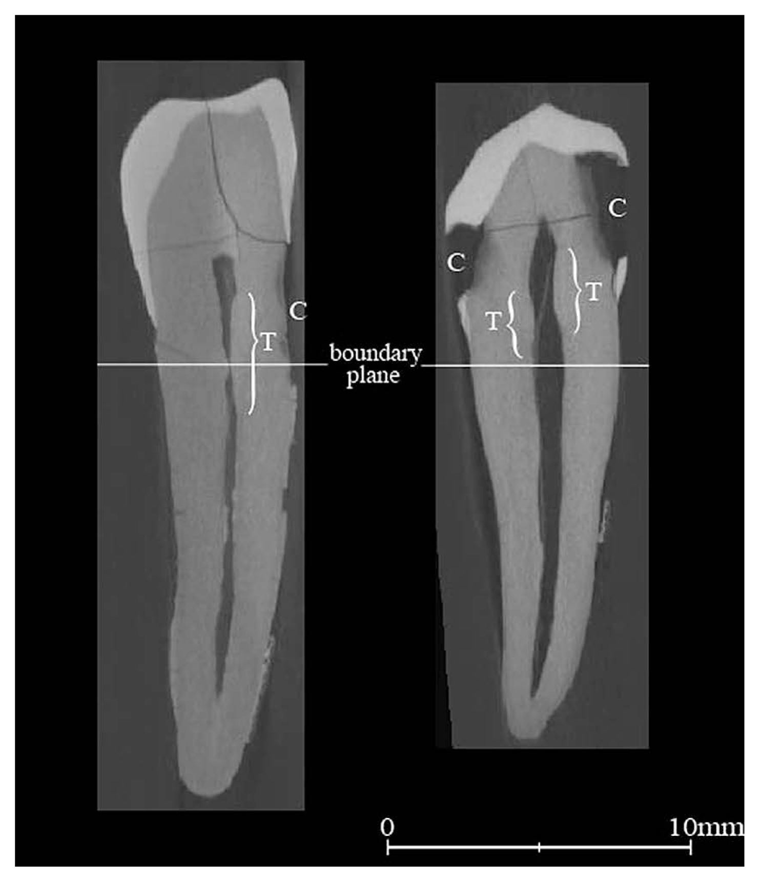
Cross-sectional CT images from labial view. Left: 70 year old female. Right: 30 year old female. C: caries, T: bulging pulp wall, which seems to be tertiary dentin induced by the corresponding caries. Below the boundary planes are the root portions defined in this study. The tertiary dentin due to cervical carries (left) affects the root portion, while that due to caries on the enamel part only (right) has little effect on the root portion.

Furthermore, we tested the difference among the sub-sample groups in each age category. Since those sub-sample groups were collected at different periods (K: 1880s–1920s; F: 1940s–1950s; M: 1970s and later), a secular change in the PVRrt reduction pattern was suspected among them. When all three sub-sample groups had more than two samples in an age category, testing was performed by one-way analysis of variance; otherwise, a t-test was performed. Due to an insufficient number of samples, the age category 20 29 could not be tested. Only male samples were used for those tests.

From Bayes’ theorem, the probability of being a certain age a conditional on having a certain PVRrt value P can be described as follows:

  

$$\text{Pr}(a\mid P)=\frac{\text{Pr}(a)·\text{Pr}(P\mid a)}{\text{Pr}(P)},$$(1)

where Pr(A) denotes the probability of A, and Pr(A | B) denotes the probability of A conditional on B. Since P is a continuous variable and a was assumed also continuous in this study, another version of equation (1) in the form of a probability density function (PDF) was preferable. Let e(a| P) be a PDF of a conditional on P, f(a) be a PDF of a, and l(P | a) be a PDF of P conditional on a. The probability density function of P can be calculated as ${\int }_0^{\infty }f(a)·l(P\mid a)·da$. Then, equation (1) becomes:

  

$$e(a\mid P)=\frac{f(a)·l(P\mid a)}{{\int }_0^{\infty }f(a)·l(P\mid a)·da}.$$(2)

The ultimate objective of this study is acquiring the left-hand side of equation (2), i.e. the probability density of age a when PVRrt was observed to be P (posterior PDF). To accomplish this, f(a) and l(P | a) are required. As f(a) (prior PDF), we assumed the age structure of Japanese population in 2012 published by the Statistics Bureau, Ministry of International Affairs and Communications, Japan (2013). Since age was a discontinuous variable in the referenced data, the PDF was approximated by a kernel density estimation with three-year bandwidth (Figure 3). After the density estimation for the whole age range, the density for age below 15 was reset to be ‘zero,’ for we did not have canine data for the corresponding age range. The effect of this resetting will be discussed later. As the prior distribution, researchers have used several forms of probability distribution. Langley- Shirley and Jantz (2010) used age-distribution data obtained from the Forensic Anthropology Data Bank (FDB) for the prior distribution in their age-estimation calculation from clavicles. Although we admit that the best choice for the prior distribution is the age distribution of the victims in actual forensic cases, data such as FDB for Japanese population is not currently available. The age distribution of missing persons was available and could have been used as prior distribution. In this case, however, we could not accept it unless the probability of becoming a victim in a forensic case is constant among all ages in the missing persons population. Adopting the Japanese age structure for the prior distribution means that we assumed an equal probability of becoming a victim (unidentified body) in a forensic case for every single Japanese (≥15 years old). As for l(P | a), we made a statistical model to describe the likelihood. We assumed PVRrt distribution conditional on a certain age to be normal and expanded it for the whole age range, where the average of the normal distribution (M) should follow an exponential curve as age increases. We created three parameters to specify the exponential curve: α determines the shape of the curve, β determines the parallel translation towards the age axis, and γ determines the parallel translation towards the PVRrt axis. Thus, the function is written as:

Figure 3

Japanese age structure as of 2012 reported by Statistics Bureau, Ministry of International Affairs and Communications, Japan (2013). The female population is stacked on the male one. Based on kernel density estimation, the probability density function (PDF) of age was approximated from the data: solid line for males and dashed line for females (these were multiplied by each gender’s total population, and the female one was stacked on the male one just to fit with the histograms in this figure). Then, PDFs for <15 years were set to zero, because of the deficiency of canine data for the corresponding range.

  

$$M=\text{exp}[\alpha ·(age-\beta )]+\gamma .$$(3)

Letting δ denote the function value at age = 15 (i.e. the initial PVRrt average), β can be expressed as $\beta =15-\text{ln}{(\delta -\gamma )}^{\frac{1}{\alpha }}$. Then, equation (3) becomes:

  

$$M=(\delta -\gamma )\text{exp}[\alpha ·(age-15)]+\gamma .$$(4)

As age goes to infinity, the function value M approaches γ. These three parameters (α, γ, δ) plus the standard deviation of the normal distribution around the curve (σ) (which was assumed to be constant across the entire age range), describe the likelihood at any age (l(P | a); here, the variable ‘age’ was substituted by a) as:

  

$$\begin{array}{l}l(P\mid a)=\frac{1}{\sqrt{2\pi }·\sigma ·q}\text{exp}\left[-\frac{1}{2}{\left(\frac{P-M}{\sigma }\right)}^2\right]\\ l(P\mid a)=0\hspace{0.17em}(\text{when\hspace{0.17em}P}>1\hspace{0.17em}\text{or\hspace{0.17em}}<0),\end{array}$$(5)

where $q={\int }_0^1\frac{1}{\sqrt{2\pi }·\sigma }\text{exp}\left[-\frac{1}{2}{\left(\frac{x-M}{\sigma }\right)}^2\right]·dx$. The normal distribution was truncated as seen in equation (5) since the probability of PVRrt being >1 or <0 is 0. α and δ were shared by males and females while γ and σ were set to vary between males and females (γ_m, γ_f, σ_m, σ_f). Thus, in total six parameters (α, γ_m, γ_f, δ, σ_m, σ_f) were determined simultaneously by the maximum likelihood method fitting the model to the observed data. Another possible model that takes the logarithm of PVRrt was not appropriate as the log PVRrt data did not show a normal distribution or a linear transition with age.

In order to assess the goodness of fit, we tested the normality of the distributions and the stability of the variances through the age range, for males and females separately. For normality, the distributions of residuals (signed distances of observed PVRrt values from the fitted exponential curve) were tested by the Kolmogorov–Smirnov test. For variance stability, the squares of those residuals were tested by the Kruskal–Wallis test among the above-mentioned age categories.

After obtaining e(a | P) from equation (2), we calculated the mean and prediction intervals of e(a | P). The X% prediction interval was defined here so that the probabilities of being above as well as below the interval are each (100 − X)/2%. X = 90, 70, or 50. Those results are depicted in what we refer to as ‘age-estimation chart.’

The age-estimation chart was compared with age- estimation charts derived in three different ways: from a Bayesian approach with uniform prior distribution; from a Bayesian approach with the age distribution of a modern hunter-gatherer as the prior distribution; and from inverse regression analysis. Only male charts were considered for simplicity. The uniform distribution was set here as that which equally distributes in the age range of 15–80 years (i.e. PDF = 1/65 for 15 ≤ age ≤ 80, PDF = 0 for any other range). To exemplify the age distribution of male hunter- gatherers, we used the data for the age-sorted number of deaths in a modern hunter-gatherer population, the !Kung, reported by Howell (Howell, 1979: Table 4.3). We fitted the survival model of Gompertz (Gompertz, 1825; Wood et al., 2002) to the reported data and used the survival function as the prior age distribution (not the distribution of death). As to the age estimation by inverse regression, we took a non-parametric approach rather than simple linear regression. Since our age data vs. PVRrt values did not show a linear transition, using simple linear regression would unnecessarily have deteriorated the age estimation by inverse regression, making the comparison unfair. The mean predicted age at a given PVRrt value was calculated as the mean age of the samples whose PVRrt values are within a window, which was set ±0.005 from the given PVRrt value. This non-parametric regression is free from the assumption of linearity for the distribution. In addition, a 70% prediction interval was defined as the age range limited by the 85th percentile value for the upper and the 15th percentile value for the lower, of the samples within the same window. The obtained curves of the mean and 70% prediction interval were smoothed three times by averaging each curve with the same window.

Finally, we compared the precision of the age estimation from PVRrt with another age-estimation method that used the os pubis. It is widely known that the morphology of the pubic symphyseal face changes with age. Brooks and Suchey (1990) studied the change using a large number of samples (n = 1225) and established a pattern for the change, which was divided into six phases. The frequencies of the six phases according to sample age were reported in their paper (Brooks and Suchey, 1990: Figure 4). We counted the frequencies, which were depicted as histograms for males and females. (At some age points, the male histogram was hidden by the female histogram; in such cases, the same frequency of males and females was assumed.) Then, the likelihood (i.e. the probability of being in a certain phase of pubic symphysis conditional on being at a certain age, which is equivalent to l(P/a) in equation (2)) was calculated according to the method described in Love and Müller (2002) (where it is called the ‘weight function’) with a bandwidth of 9 years. This method non-parametrically produces the likelihood from age-sorted frequency data after smoothing the frequency distribution. Thereafter, as the case of PVRrt, the posterior PDF (i.e. the probability density of being a certain age when a certain os pubis phase was observed) was calculated using Bayes’ theorem with the 2012 Japanese population data (Statistics Bureau, Ministry of International Affairs and Communications, Japan, 2013) as the prior. To compare the results from the two different age-estimation methods, expectations of the prediction intervals were calculated to represent the degree of precision of each estimation method. To do so, first, the marginal PDF of PVRrt (and the marginal probability of each phase in the Suchey–Brooks system) in the Japanese population was calculated. The marginal PDFs of PVRrt are therefore a theoretically estimated PVRrt distribution in the Japanese population, which was calculated as the denominator in equation (2). When the prediction intervals (upper limit minus lower limit) are averaged across the whole range of PVRrt being weighed by the marginal distribution, this provides values that represent the expectations of the prediction intervals when numerous age- estimation trials were repeated in the Japanese population, and the same can be said for those of the Suchey–Brooks estimation. Specifically, the expectations were calculated in the following way: the upper limit minus the lower limit of X% prediction interval for a PVRrt value (or for a Suchey–Brooks phase) multiplied by the marginal probability density (or the marginal probability) was integrated across the entire PVRrt range (or summed across all the six phases).

We used the computer software packages R 2.13.0 (R Development Core Team, 2011) for statistical analyses and MATLAB (R2010b) (MathWorks, Natick, USA) for mathematical computations.

For all statistical tests, we set the significance level at 0.05.

Results

The means of PVRrt and the test results among age and sex categories are shown in Table 2. Generally, PVRrt decreases with age for both sexes. Nevertheless, a decrease after age 50 was not recognizable for males. While there was no significant difference between sexes in the younger categories (15–19, 20–29, and 30–39), female values tended to be significantly lower than the males in the older categories (>40, except 50–59).

Table 2 Means of PVRrt1 for each sex and age category, and the results of t-tests among them

	15–19		20–29		30–39		40–49		50–59		60–69		≥70
Male mean (in %) and inter-age category comparison	7.10	**	5.67	**	4.61	NS (0.63)2	4.48	**	3.83	NS (0.98)	3.82	NS (0.59)	3.96
Inter-sex comparison	NS (0.95)		NS (0.43)		NS (0.76)		**		NS (0.31)		**		**
Female mean (in %) and inter-age category comparison	7.06	*	5.47	**	4.50	*	3.62	NS (0.84)	3.55	*	2.94	NS (0.07)	2.57

1  Pulp volume ratio within the root portion of lower canine.

2  Numbers in parentheses show the P values when the tests were not significant at a significance level of 0.05.

*  P < 0.05;

**  P < 0.01.

See Table 1 for the numbers of the samples.

No significant difference was found in the comparison between specimens with and without cervical lesions in any age category (all P values ≥ 0.23), but there was a tendency that those with cervical lesions had slightly smaller mean values than those without them (Table 3).

Table 3 Comparison between teeth with and without cervical lesion (using male samples only)

	40–49	50–59	60–69	≥70	≥ 50 (combined)
Mean PVRrt (%)
without cervical lesion	4.61 (n = 23)	3.67 (n = 19)	3.93 (n = 21)	3.99 (n = 24)	3.87 (n = 64)
with cervical lesion	4.14 (n = 9)	4.07 (n = 12)	3.56 (n = 9)	3.88 (n = 8)	3.86 (n = 29)
Difference (without–with)	0.47	−0.4	0.37	0.11	0.01
P value (t-test)	0.23	0.26	0.30	0.80	0.95
95% confidence interval of the difference	−0.33~1.27	−1.13~0.32	−0.34~1.08	−0.81~1.03	−0.41~0.44

In the age range of 15–39 there were not enough samples with cervical lesions for a statistical test.

The results of the tests for secular trends in the sub-sample groups are shown in Table 4. None of the age categories showed any significant difference among the three sub sample groups.

Table 4 Tests for the difference in PVRrt among three sub-sample groups to see any secular trend (using male samples only)

	15–19	20–29	30–39	40–49	50–59	60–69	≥70
Test conducted	t-test	test was not available	one-way ANOVA	t-test	one-way ANOVA	one-way ANOVA	one-way ANOVA
Number of samples (K, F, M)	(11, 7, 0)	(32, 0, 1)	(19, 7, 7)	(21, 0, 11)	(12, 8, 11)	(3, 19, 8)	(2, 24, 6)
P value	0.86	—	0.54	0.41	0.16	0.76	0.76
Judge	NS	—	NS	NS	NS	NS	NS

Sub-sample group K was collected in 1880s–1920s, F was 1940s–1950s, M was 1970s or later.

Figure 4 shows the results of fitting the exponential curve model to the observed data, and the slopes of the curves. The parameters resulting from the fitting are summarized in Table 5. Scatter plots of the residuals against age and their distributions are shown in Figure 5. The Kolmogorov–Smirnov test did not reject the hypothesis that the observations of the residuals followed the normal distribution with mean = 0 and SD = sample SD, for both sexes (P = 0.28 for males, 0.98 for females). The Kruskal–Wallis test did not indicate significant inequality in the residual variation among those age categories, for both sexes (P = 0.08 for male, 0.41 for female). The nearly significant result of males seemed mainly caused by the relatively large variation in the 15–19 category as the P value became 0.41 when that category was eliminated from the test. The variations (calculated as $\sqrt{\frac{1}{n}\sum {(residual)}^2}$) for each age category are shown in Figure 5 in parentheses.

Figure 4

Scatter diagram of PVRrt (pulp volume ratio within the root portion) vs. age and the exponential curve model fitted to the data On the top are the slopes of the fitted curves. According to this model, PVRrt normally distributes around a exponential curve. The model was fitted so that the curves for males and females share the index on Napier’s constant and the initial point at age 15, but the asymptotic line and variation for the normal distribution were different between them. The fitting method was the maximum likelihood method.

Table 5 Parameters of the statistical model determined by maximun likelihood method

	α	γ	δ	σ
Male	−5.17 × 10−2	3.49 × 10−2	7.36 × 10−2	1.085 × 10−2
Female	−5.17 × 10−2	2.58 × 10−2	7.36 × 10−2	0.904 × 10−2

α, shape factor of the curve (shared by male and female); γ, asymptotic line; δ, initial value at age 15 (shared by male and female); σ, σ of normal distribution.

Figure 5

Scatter diagrams of residuals and their histograms, for males and females. Residuals are signed distances of PVRrt observations from the fitted exponential curves (see Figure 4). The curves on the histograms are the normal distribution of mean = 0, SD = sample SD. The parentheses indicate deviation of the residuals in each age category calculated as $\sqrt{\frac{1}{n}\sum {(residual)}^2}$.

Figure 6 shows the age-estimation charts based on PVRrt for the Japanese population. There are three charts for targets known to be male, female, or gender unknown. Mean prediction line, and 50%, 70%, and 90% prediction intervals of the estimated age are drawn across a PVRrt range of 0–0.11 in each chart. Above those charts are the marginal PDFs of PVRrt in the Japanese populations, calculated as described above.

Figure 6

Age-estimation charts for males, females, and gender-unknown for the modern Japanese population. Mean prediction line, and 50%, 70%, 90% prediction intervals were drawn across a PVRrt range of 0–0.11. The PDF curve above each chart is the marginal PDF of PVRrt, indicating the distribution of PVRrt in modern Japanese males, females, and total population.

The age-estimation charts obtained with uniform prior and (approximated) !Kung prior and by inverse regression are shown in Figure 7. On the right-upper corner of each chart is the prior distribution used for the Bayesian approach or the age distribution of the samples used for the inverse regression. The right-lower sub-figure shows the mean pre -diction lines of those estimation charts all superimposed; those are Bayesian with modern-Japanese prior, Bayesian with uniform prior, Bayesian with !Kung prior, and estimation by inverse regression. While the mean lines of Bayesian with modern-Japanese, Bayesian with uniform, and inverse regression are similar (the mean line of inverse regression in the range PVRrt < 0.03 or PVRrt > 0.08 should be disregarded due to the deficiency of the sample), that of Bayesian with !Kung prior deviated widely from the others.

Figure 7

Age-estimation charts obtained with uniform prior (top left), approximated male !Kung prior (top right), and by inverse regression method (bottom left). Likelihoods used for both Bayesian approaches were those of males. The circles in the bottom left indicate male samples used in the calculation. Both sides of the mean prediction line and the 70% prediction interval obtained by inverse regression were made light-colored and should be disregarded due to the lack of samples for the calculation. On the right upper corner of each chart is the prior distribution used for the Bayesian approach or the age distribution of the samples used for the inverse regression. The dashed line on the !Kung distribution indicates the survival curve reconstructed from the reported data (Howell, 1979: Table 4.3), and the solid line is the fitted Gompertz curve. Bottom right shows the mean prediction lines of those charts plus the chart obtained with modern male Japanese prior (Figure 6), all superimposed together.

The likelihood distribution used for the calculation of posterior PDF from the Suchey–Brooks phase system are shown in Figure 8. The likelihood for each phase can be obtained by drawing a vertical line at any age on the figure and measuring the length of each phase section. The age- estimation charts based on the Suchey–Brooks phase system are shown with mean values and prediction intervals in Figure 9. Above those charts are the marginal probability for each phase. As explained above, expectations of the prediction intervals were calculated for both PVRrt and the Suchey–Brooks method, and those results are compared in Table 6. The expectations are generally larger for the PVRrt method than for the Suchey–Brooks method, but were comparable between the methods when the target was female.

Figure 8

Likelihood of having a certain Suchey–Brooks phase on an os pubis vs. age. Vertical section at any age indicates the probabilities of having those phases at that age. These were calculated according to Love and Müller (2002) from the frequency data in Brooks and Suchey (1990). It is likely that the humps of phase IV and V seen in the old ranges are merely reflecting random fluctuations due to the deficient number of samples in the original data for that range, since it is unlikely that younger phases will increase their frequencies compared to older ones as age increases.

Figure 9

Age-estimation charts based on the Suchey–Brooks os pubis phase for the Japanese population. For each phase, we calculated PDF of the estimated age from the likelihood data shown in Figure 7 with the Japanese population data by using Bayes’ theorem, and obtained the mean and predicted intervals from the PDF. Unlike in Figure 6, the dashed lines are merely connecting the prediction intervals of neighboring phases. The probability distribution above each chart is the marginal probability distribution of Suchey–Brooks phases in modern Japanese males, females, or the total population.

Table 6 Comparison between the two methods based on expectations of the prediction intervals

	Male			Female			Gender unknown
	50%	70%	90%	50%	70%	90%	50%	70%	90%
PVRrt method (years)	22.0	32.8	48.8	19.9	30.0	45.1	21.4	32.2	48.1
1 Suchey–Brooks method (years)	14.8	23.1	39.4	19.0	29.1	43.1	16.2	26.8	42.4

1  Calculated from data in Brooks and Suchey (1990).

Discussion

Analysis among age and sex categories indicated that there is a difference in the rate of decrease of PVRrt between males and females. In females, the value decreased more rapidly than in males. One can also recognize this tendency by referring to the scatter diagram and the fitted curves in Figure 4. Although the reason for the difference is not clear, it could be because of some direct or indirect factors. Plausible direct factors include differences in the tooth shape and size, which influence the number of odontoblasts per root volume, or differences in gene expression of odontoblasts, which affect the degree of dentin secretion. Indirect factors include differences in hormonal homeostasis, oral environment, and masticatory stresses. Since teeth with or without cervical lesions did not have large differences (see the confidence intervals in Table 3) compares to the sex differences, the presence or absence of lesions such as caries cannot be the major cause of the sex difference.

In any age category, the tests for the differences in PVRrt between teeth with and without cervical lesions presented no statistical significance (Table 3). The 95% confidence interval for the difference was from −0.41 to 0.44% for the age category ≥50. The standard deviation of PVRrt can be approximated as the σ in the fitted statistical model shown in Table 5, which were 1.085 × 10⁻² for males and 0.904 × 10⁻² for females. By comparing the 1 SD range to the 95% confidence interval, one can recognize that the difference due to the cervical lesions possibly accounts for roughly 40–50% of the 1 SD range of PVRrt; this difference is not negligible. The other age categories would have given no better results with even wider confidence intervals. Therefore, although no significant difference was observed in those tests, we could not conclude that the difference was negligibly small. We agree that this issue needs further research with a sufficient number of samples for such age-sorted types of analysis. In the other subjects in this study, the possible difference induced by cervical lesions was not considered.

As tests for the secular trend in PVRrt reduction did not show differences, we considered that those three sub-sample groups could be treated as one. Furthermore, as the last collected sub-sample group was recent (1970s or later), we assumed the same PVRrt reduction pattern as for the current Japanese population.

Although the test for equality of the variation fell close to the significance level in males( P = 0.08), variation along the model exponential curve was treated as constant in this study. While the statistical model adopted in this study may not thoroughly describe the nature of PVRrt reduction, we supposed that the model was good enough to approximate the probability distribution of PVRrt, at least across the adult age range of studied samples. The reason why teenage samples exhibited a relatively large variation might be the difference in the initiation time of odontogenesis. A slight difference of the time should cause large differences when PVRrt reduction is still rapid.

The age-estimation charts in Figure 6 exhibit some noteable features. The prediction intervals in the male chart are generally wider than those in the female chart. This is, in part, because, as seen in Figure 4, the slope of the female curve is steeper than that of the male curve. Assuming the variance of PVRrt around the slope is unchanged, the steeper the slope becomes, the more it should confine the probable age range for a PVRrt value. The slightly larger value of σ in males could also be one of the reasons for the difference. Another significant point is that the mean curve tends to be younger in males than in females as it goes left of the charts. This is a manifestation of the difference in life expectancies between males and females also seen in the modern Japanese population. In particular, when the population is confined younger than that of females, because females tend to live longer than males. A low PVRrt value has the same effect as confining the probable age to old, and therefore the average age of males becomes younger than that of females.

What should be kept in mind is that the probability of being below age 15 was forced to be zero since the population frequency for that range was set to zero during the calculations. According to Moorrees et al. (1963), the age of root apex completion for lower canines is, approximately, 10–16 years for males and 9–14 years for females. Thus, root maturation does not necessarily confirm that the person is at or over 15. Therefore, technically, using this chart requires verification that the target individual is ≥15 years by any other (rough) age information, especially when the estimated age by PVRrt is close to 15.

When several prior distributions and inverse regressions are compared, it can be said that the results (especially the mean prediction lines) are similar among male Japanese prior, uniform prior, and inverse regression. The reason the inverse regression and the uniform prior had similar results (values in the range 0.08 < PVRrt < 0.03 were disregarded) is because the underlying age distributions were similar between them, i.e. the male sample distribution used in the present study was similar to the 15–80 uniform distribution. This is an indication that inverse regression methods can be used when the target has a similar age distribution to the reference sample. As far as PVRrt age estimation is concerned, the male Japanese age distribution is also rather similar to the uniform distribution, contributing to the similarity of the mean prediction curve with those of uniform prior and inverse regression (Figure 3, Figure 7). However, the male !Kung (approximate) age distribution was not similar in that sense. The difference in the mean prediction was roughly 10 years in the left half of the chart from other priors (Figure 7). This indicates that an inappropriate choice for the prior distribution can lead significant bias in the age estimation. If the prior differed from the real target distribution as much as the difference between the modern male Japanese distribution and the approximated male !Kung distribution, the error could be up to 10 years.

As seen in the result of comparison between the PVRrt method and the Suchey-Brooks method (Table 6), the former is generally inferior to the latter when the target is known to be a male or a gender unknown subject in terms of the precision of the prediction. For females, however, the precision of the PVRrt method is reasonably comparable to the Suchey–Brooks method. As indicated in Table 2, female PVRrt continues to decrease even within an old age range. As many skeletal age indicators hardly keep changing after 50 years of age, this fact is noteworthy. This is especially important when the target population is dominated by elderly people such as the modern Japanese population. Another advantage of the PVRrt method is the durability of the material. Teeth are harder and more stable against both physical and chemical degradation after death than any other part of the human skeleton; therefore the chance to apply this method will be more frequent than methods which utilize other skeletal parts. Furthermore, as an age indicator—the PVRrt value—is a continuous variable (unlike in the Suchey–Brooks phase system), so that the estimation is not the result of a limited number of outcomes, but differs each time according to the PVRrt value. Considering these advantages, we conclude that the PVRrt method is a useful age-estimation method in forensic cases especially when the victim is known to be a female.

Conclusion

Using a Bayesian approach, we provided sex-dependent charts for human age estimation from pulp volume reduction of the lower canine teeth. The precision of estimation was not better than that of widely used skeleton-based age-estimation methods such as the Suchey–Brooks pubic symphysis method. However, this method will demonstrate its value when the victim’s body is highly decomposed and many crucial skeletal parts are missing. An observed pulp volume ratio in the lower canine root from modern Japanese population can be converted into the estimated age with prediction intervals by referring to Figure 6 in this paper.

Acknowledgments

We are grateful to Gen Suwa, Eisaku Kanazawa, Yasuhisa Tsujimoto, Mitsuko Nakayama, and Yoko Wada for kindly accommodating our needs for tooth specimens. We also wish to thank the staff of the Paleoanthropology Laboratory, The University Museum, The University of Tokyo and of Skeletal Biology & Anthropology Laboratory, Graduate School of Science, The University of Tokyo for their support and advice.

References

•  Aboshi  H.,  Takahashi  T., and  Komuro  T. (2010) Age estimation using microfocus X-ray computed tomography of lower pre-molars. Forensic Science International, 200: 35–40.
•  Agematsu  H.,  Someda  H.,  Hashimoto  M.,  Matsunaga  S.,  Abe  S.,  Kim  H.J.,  Koyama  T.,  Naito  H.,  Ishida  R., and  Ide  Y. (2010) Three-dimensional observation of decrease in pulp cavity volume using micro-CT: age-related change. Bulletin of Tokyo Dental College, 51: 1–6.
•  Bocquet-Appel  J.P. and  Masset  C. (1982) Farewell to paleodemogzaphy. Journal of Human Evolution, 11: 321–333.
•  Bosmans  N.,  Ann  P.,  Aly  M., and  Willems  G. (2005) The application of Kvaal’s dental age calculation technique on panoramic dental radiographs. Forensic Science International, 153: 208–212.
•  Brooks  S. and  Suchey  J.M. (1990) Skeletal age determination based on the os pubis: a comparison of the Acsádi-Nemeskéri and Suchey-Brooks methods. Human Evolution, 5: 227–238.
•  Buckberry  J.L. and  Chamberlain  A.T. (2002) Age estimation from the auricular surface of the ilium: a revised method. American Journal of Physical Anthropology, 119: 231–239.
•  Burns  K.R. and  Maples  W.R. (1976) Estimation of age from individual adult teeth. Journal of Forensic Sciences, 21: 343–356.
•  Cameriere  R.,  Ferrante  L.,  Belcastro  M.G.,  Bonfiglioli  B.,  Rastelli  E., and  Cingolani  M. (2007) Age estimation by pulp/tooth ratio in canines by peri-apical X-rays. Journal of Forensic Sciences, 52: 166–170.
•  Cameriere  R.,  Cunha  E.,  Wasterlain  S.N.,  De Luca  S.,  Sassaroli  E.,  Pagliara  F.,  Nuzzolese  E.,  Cingolani  M., and  Ferrante  L. (2013) Age estimation by pulp/tooth ratio in lateral and central incisors by peri-apical X-ray. Journal of Forensic and Legal Medicine, 20: 530–536.
•  Coqueugniot  H.,  Weaver  T.D., and  Houët  F. (2010) Brief communication: a probabilistic approach to age estimation from infracranial sequences of maturation. American Journal of Physical Anthropology, 142: 655–664.
•  Dalitz  G.D. (1962) Age determination of adult human remains by teeth examination. Journal of the Forensic Science Society, 3: 11–21.
•  Du  C.,  Zhu  Y., and  Hong  L. (2011) Age-related changes in pulp cavity of incisors as a determinant for forensic age identification. Journal of Forensic Sciences, 56: S72–S76.
•  Drusini  A.G. (2008) The coronal pulp cavity index: a forensic tool for age determination in human adults. Cuademos de Medicina Forense, 14: 235–249.
•  Drusini  A.G.,  Toso  O., and  Ranzato  C. (1997) The coronal pulp cavity index: a biomarker for age determination in human adults. American Journal of Physical Anthropology, 103: 353–363.
•  Gompertz  B. (1825) On the nature of the function expressive of the law of human mortality, and on a new mode of determining the value of life contingencies. Philosophical Transactions of the Royal Society of London (Series A), 115: 513–583.
•  Gowland  R.L. and  Chamberlain  A.T. (2002) A Bayesian approach to aging perinatal skeletal material from archaeological sites: implications for the evidence for infanticide in Roman-Britain. Journal of Archaeological Science, 29: 677–685.
•  Gustafson  G. (1950) Age determinations on teeth. Journal of the American Dental Association, 41: 45–54.
•  Hoppa  R.D. and  Vaupel  J.W. (2002) The Rostock manifesto for paleodemography: the way from stage to age. In:  Hoppa  R.D. and  Vaupel  J.W. (eds.), Paleodemography: age Distributions from Skeletal Samples. Cambridge University Press, Cambridge, pp. 1–8.
•  Howell  N. (1979) Demography of the Dobe !Kung, Academic Press, New York.
•  Johanson  G. (1971) Age determinations from human teeth. Odontologiski Revy, 22 (Supplement 21): 1–126.
•  Kashyap  V.K. and  Koteswara Rao  N.R. (1990) A modified Gustafson method of age estimation from teeth. Forensic Science International, 47: 237–247.
•  Kimmerle  E.H.,  Konigsberg  L.W.,  Jantz  R.L., and  Baraybar  J.P. (2008) Analysis of age-at-death estimation through the use if pubic symphyseal data. Journal of Forensic Sciences, 53: 558–568.
•  Kolltveit  K.M.,  Solheim  T., and  Kvaal  S.I. (1998) Methods of measuring morphological parameters in dental radiographs. Comparison between image analysis and manual measurements. Forensic Science International 94: 87–95.
•  Konigsberg  L.W.,  Herrmann  N.P.,  Wescott  D.J., and  Kimmerle  E.H. (2008) Estimation and evidence in forensic anthropology: age-at-death. Journal of Forensic Sciences, 53: 541–557.
•  Kvaal  S. and  Solheim  T. (1994) A non-destructive dental method for age estimation. Journal of Forensic Odonto-Stomatology, 12: 6–11.
•  Kvaal  S.I.,  Kolltveit  K.M.,  Thomsen  I.O., and  Solheim  T. (1995) Age estimation of adults from dental radiographs. Forensic Science International, 74: 175–185.
•  Landa  M.I.,  Garamendi  P.M.,  Botella  M.C., and  Alemán  I. (2009) Application of the method of Kvaal et al. to digital orthopantomograms. International Journal of Legal Medicine, 123: 123–128.
•  Langley-Shirley  N. and  Jantz  R.L. (2010) A Bayesian approach to age estimation in modern Americans from the clavicle. Journal of Forensic Sciences, 55: 571–583.
•  Love  B. and  Müller  H.G. (2002) A solution to the problem of obtaining a mortality schedule for paleodemographic data. In:  Hoppa  R.D. and  Vaupel  J.W. (eds.), Paleodemography: Age Distributions from Skeletal Samples. Cambridge University Press, Cambridge, pp. 181–192.
•  Lucy  D.,  Aykroyd  R.G.,  Pollard  A.M., and  Solheim  T. (1996) A Bayesian approach to adult human age estimation from dental observations by Johanson’s age changes. Journal of Forensic Sciences, 41: 189–194.
•  Maples  W.R. (1978) An improved technique using dental histology for estimation of adult age. Journal of Forensic Sciences, 23: 764–770.
•  Maples  W.R. and  Rice  P.M. (1979) Some difficulties in the Gustafson dental age estimations. Journal of Forensic Sciences, 24: 168–172.
•  Meinl  A.,  Tangl  S.,  Pernicka  E.,  Fenes  C., and  Watzek  G. (2007) On the applicability of secondary dentin formation to radiological age estimation in young adults. Journal of Forensic Sciences, 52: 438–441.
•  Moorrees  C.F.A.,  Fanning  E.A., and  Hunt  E.E., Jr. (1963) Age variation of formation stages for ten permanent teeth. Journal of Dental Research, 42: 1490–1502.
•  Nagaoka  T.,  Sawada  J., and  Hirata  K. (2008) Did the Jomon people have a short lifespan? Evidence from the adult age-at-death estimation based on the auricular surface of the ilium. Anthropological Science, 116: 161–169.
•  Nagaoka  T.,  Abe  M., and  Shimatani  K. (2012a) Estimation of mortality profiles from non-adult human skeletons in Edo-period Japan. Anthropological Science, 120: 115–128.
•  Nagaoka  T.,  Ishida  H.,  Shimoda  Y.,  Sunagawa  M.,  Amano  T.,  Ono  H., and  Hirata  K. (2012b) Estimation of skeletal adult age distribution of Okhotsk people in northern Japan. Anthropological Science, 120: 103–113.
•  Paewinsky  E.,  Pfeiffer  H., and  Brinkmann  B. (2005) Quantification of secondary dentine formation from orthopantomograms—a contribution to forensic age estimation methods in adults. International Journal of Legal Medicine, 119: 27–30.
•  Prince  D.A. and  Konigsberg  L.W. (2008) New formulae for estimating age-at-death in the Balkans utilizing Lamendin’s dental technique and Bayesian analysis. Journal of Forensic Sciences, 53: 578–587.
•  Prince  D.A.,  Kimmerle  E.H., and  Konigsberg  L.W. (2008) A Bayesian approach to estimate skeletal age-at-death utilizing dental ware. Journal of Forensic Sciences, 53: 588–593.
•  Someda  H.,  Saka  H.,  Matsunaga  S.,  Ide  Y.,  Nakahara  K.,  Hirata  S., and  Hashimoto  M. (2009) Age estimation based on three- dimensional measurement of mandibular central incisors in Japanese. Forensic Science International, 185: 110–114.
•  Spoor  C.F.,  Zonneveld  F.W., and  Macho  G.A. (1993) Linear measurements of cortical bone and dental enamel by computed tomography: applications and problems. American Journal of Physical Anthropology, 91: 469–484.
•  Star  H.,  Thevissen  P.,  Jacobs  R.,  Fieuws  S.,  Solheim  T., and  Willems  G. (2011) Human dental age estimation by calculation of pulp-tooth volume ratios yielded on clinically acquired cone beam computed tomography images of monoradicular teeth. Journal of Forensic Sciences, 56: S77–S82.
• Statistics Bureau, Ministry of International Affairs and Communications, Japan (2013) Current population estimates as of 1 October 2012. Retrieved 1 July 2013 from: www.e-stat.go.jp/SG1/estat/ListE.do?lid=000001109855
•  Storey  R. (2007) An elusive paleodemography? A comparison of two methods for estimating the adult age distribution of deaths at late classic Copan, Honduras. American Journal of Physical Anthropology, 132: 40–47.
•  Thevissen  P.W.,  Fieuws  S., and  Willems  G. (2010) Human dental age estimation using third molar developmental stages: does a Bayesian approach outperform regression models to discriminate between juveniles and adults? International Journal of Legal Medicine, 124: 35–42.
•  Vandevoort  M.,  Bergmans  L.,  Cleynenbreugel  J.V.,  Bielen  D.J.,  Lambrechts  P.,  Wevers  M.,  Peirs  A., and  Willems  G. (2004) Age calculation using X-ray microfocus computed tomographical scanning of teeth: a pilot study. Journal of Forensic Sciences, 49: 787–790.
•  Willems  G.,  Moulin-Romsee  C., and  Solheim  T. (2002) Non-destructive dental-age calculation methods in adults: intra- and inter-observer effects. Forensic Science International, 126: 221–226.
•  Wood  J.W.,  Holman  D.J.,  O’connor  K.A., and  Ferrell  R.J. (2002) Mortality models for paleodemography. In:  Hoppa  R.D. and  Vaupel  J.W. (eds.), Paleodemography: Age Distributions from Skeletal Samples. Cambridge University Press, Cambridge, pp. 129–168.
•  Yang  F.,  Jacobs  R., and  Willems  G. (2006) Dental age estimation through volume matching of teeth imaged by cone-beam CT. Forensic Science International, 159S: S78–S83.