A simple method for modeling amyloid kinetics featuring position biased fiber breakage

Abstract

A mathematical model of amyloid fiber formation is described that is able to simply specify different rates of fiber breakage at internal versus end regions. This Note presents the derivation of the relevant equations and provides results showing the dramatic effects of position biased fiber breakage on the kinetics of amyloid growth.

Significance

A kinetic model of amyloid formation is presented based on two inter-related ordinary differential equations. The model can simply account for different rates of breakage at the fiber ends vs. internal regions. In the former case, breakage releases a monomer unable to maintain its amyloid structure. In the latter case, breakage produces two smaller fibers each able to act as ‘seeds’ able to facilitate amyloid growth. Thus position dependent susceptibility to breakage could determine whether breakage encourages or discourages amyloid growth. These outcomes are crucial when considering the role amyloid growth plays in disease aetiology, such as for Alzheimer’s disease.

Introduction

Protein helical polymerization reactions, such as those constituted by actin and tubulin assembly, have been a much studied topic in biophysics [1,2]. Amyloid, a fibril-like homopolymer capable of being formed from many different protein monomer building blocks, has been shown to exhibit both helical polymerization kinetics and steady state behavior capable of quantitative description using helical polymerization models of Oosawa and colleagues [3–6]. A number of important extensions to these models been developed over the last twenty years to better describe amyloid formation [7–14]. These extensions are based on a consensus chemical schema (Fig. 1) featuring the following three general processes, (i.) Reversible fiber nucleation; (ii.) Fiber growth and dissolution via monomer addition and loss; and (iii.) Fiber breakage and joining. A simple kinetic description containing some aspects of the consensus mechanism was developed by Smith, J. F., et al. [15] who employed an approach cast in terms of average quantities. Although providing less information about the time dependent evolution of the polymer distribution, this reduced model proved particularly simple to code and produced easily interpretable output. However, due to the approximations involved in its derivation, the Smith, J. F., et al. [15] model lacked the flexibility to treat biologically relevant limiting cases of amyloid fiber growth. One such important case, described by Hall and Edskes [9], was that relating to differential rates of amyloid fiber breakage from the fiber ends (to release a monomer), versus that occurring internally (to produce two shorter amyloid fibers). A recent approach based on the method of moments [16], developed a relatively complex solution to the simulation of this differential end versus internal breakage problem by approximating the evolving amyloid polymer distribution through the use of a large number (>100) of Gaussian functions. In this Letter, I derive a simpler approximate solution to the case of position dependent fiber breakage based on the assumption of a single distribution characterizing the fibril population. The current approach retains the relative simplicity of the earlier Smith, J. F., et al. [15] model without having to resort to the complex function approach adopted by Nicoud, L., et al. [16]. The method has the added benefit that it can also simply treat cases relating to differential rates of fiber end-to-end joining.

Figure 1

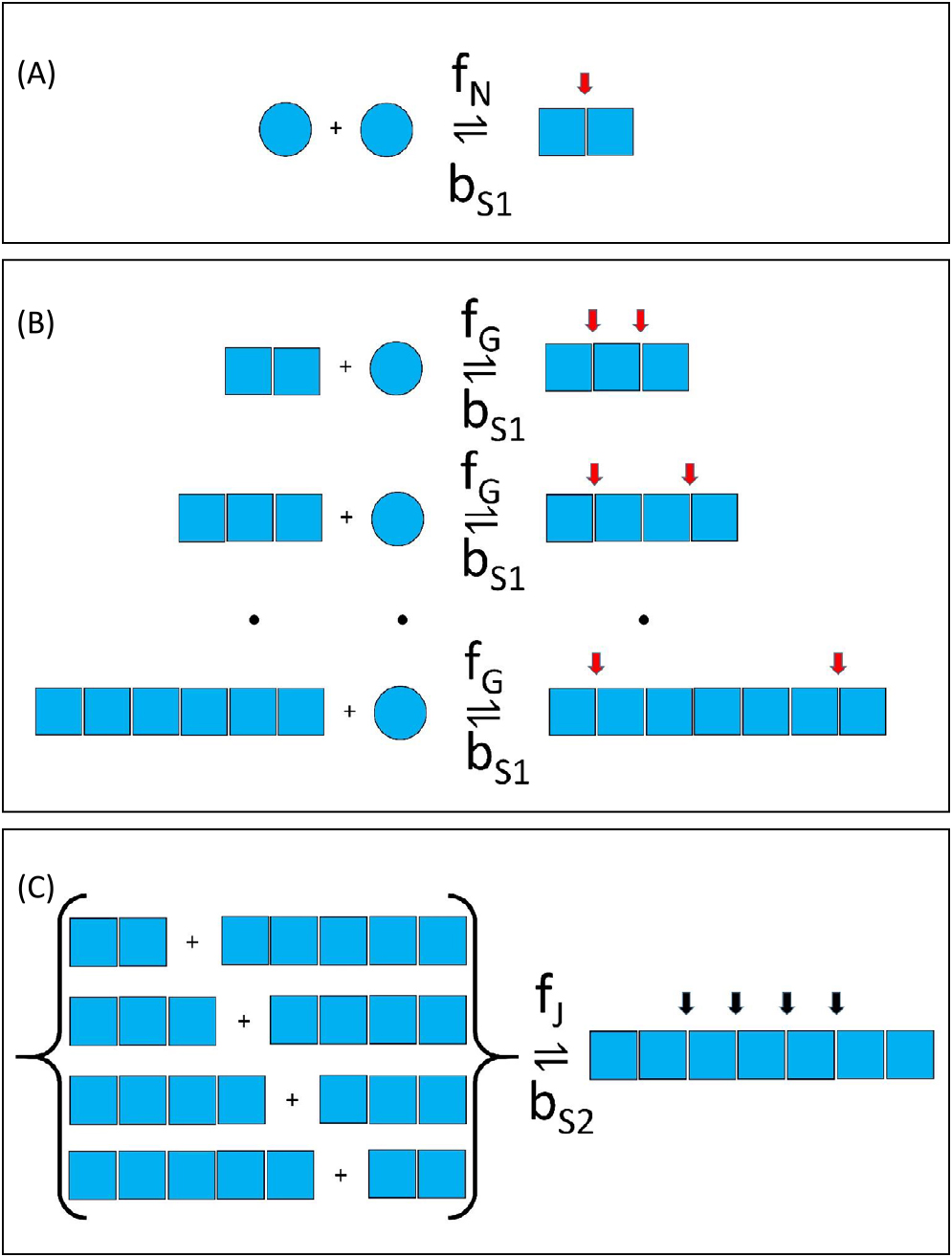
Consensus amyloid formation mechanism featuring position dependent bias in fiber breakage: (A) Nucleation—modeled as the interaction of two monomers to form a dimer nucleus with the process regulated by a second-order nucleation rate constant, f_N, (units of M^–1s^–1) and a reverse unimolecular process governed by a first-order breakage rate constant, b_S1 (units of s^–1). (B) Growth and dissolution—in which fibrils can increase in size via monomer addition, regulated by a second-order growth rate constant, f_G (units of M^–1s^–1) and decrease in size via breakage at the end of the fiber that results in monomer loss and is regulated by a first-order breakage rate constant, b_S1 (units of s^–1). (C) Fiber joining and breakage—fiber growth may also occur between any two fibers at a rate determined by the second-order rate constant, f_J (units of M^–1s^–1) and fiber internal breakage specified by a set of common site-specific intrinsic breakage rate constants, b_S2 (units of s^–1). End sites for breakage (characterized by breakage rate constant, b_S1) are shown by a red arrow. Internal sites for breakage (characterized by breakage rate constant, b_S2) are shown using a black arrow.

Theory

In developing a model of amyloid formation featuring position related breakage propensities, the following simplifying assumptions are made.

(i.) Amyloid growth follows a minimal mechanism (identical to that shown in Fig. 1), featuring fiber nucleation, fiber growth and dissolution via monomer addition/loss and fiber joining and breakage.

(ii.) The mechanism is characterized by a phenomenological fixed nucleus size set at 2 monomers along with specification of a single structural isomer type (per polymer degree) for all amyloid aggregates. Here, “phenomeno­logical” refers to the fact that we do not seek to determine the correct ‘critical nucleus size’ but rather just specify forward and reverse nucleation rates which, through their variation, can empirically accommodate experimentally observed time courses of amyloid formation whilst keeping the nucleus size set at 2.

(iii.) There are two general first-order intrinsic breakage rates: b_S1 (the end scission rate operating at terminal monomer bonds) and b_S2 (the internal scission rate operating at internalized monomer to monomer bonds) (Fig. 1).

To further develop the model three averaged quantities are defined; (C_E)_TOT—the total number concentration of ends for amyloid growth assuming uni-directional growth [17,18] (Eq. 1—where z describes the degree of the longest amyloid polymer in solution at that particular time); (C_P)_TOT—the total concentration of monomer existing within amyloid extendable form (Eq. 2), and $⟨i⟩$—the average amyloid polymer degree (Eq. 3).

  

${(C_E)}_{\mathrm{T}\mathrm{O}\mathrm{T}}=C_2+\sum _{i=3}^z{C}_i$(1)

  

${(C_P)}_{\mathrm{T}\mathrm{O}\mathrm{T}}=2C_2+\sum _{i=3}^{z}i C_i$(2)

  

$$⟨i⟩=\frac{{\left(C_P\right)}_{\mathrm{T}\mathrm{O}\mathrm{T}}}{{\left(C_E\right)}_{\mathrm{T}\mathrm{O}\mathrm{T}}}$$(3)

Chemical rate equations describing the total concentration of amyloid ends and the total concentration of polymeric amyloid species can be specified as shown in Eq. 4 and 5 (with a derivation shown in Appendix 1).

  

$$\begin{array}{ccc}\frac{d{\left(C_E\right)}_{\mathrm{T}\mathrm{O}\mathrm{T}}}{dt}\hfill & =\hfill & f_N{C}_1^2+C_2^{}\left(b_{S2}-b_{S1}\right)+b_{S2}{\left(C_P\right)}_{\mathrm{T}\mathrm{O}\mathrm{T}}\hfill \\ & & -3b_{S2}{\left(C_E\right)}_{\mathrm{T}\mathrm{O}\mathrm{T}}-f_J{{\left(C_E\right)}_{\mathrm{T}\mathrm{O}\mathrm{T}}}^2\hfill \end{array}$$(4)

  

$$\frac{d{\left(C_P\right)}_{\mathrm{T}\mathrm{O}\mathrm{T}}}{dt}=2f_N{C}_1^2-2b_{S1}{\left(C_E\right)}_{\mathrm{T}\mathrm{O}\mathrm{T}}+f_G{\left(C_E\right)}_{\mathrm{T}\mathrm{O}\mathrm{T}}{C}_1^{}$$(5)

Depending upon the nature of the simulated system the free monomer concentration, C₁, may be considered as a constant [19] or else evaluated at each time point by difference between total protein and polymerized forms based on conservation of mass principles [19]. From inspection we note that Eq. 4 requires specification of the concentration of the phenomenological nucleus, C₂. To provide a running time-dependent estimate for C₂ (alongside the time-dependent estimates of (C_E)_TOT, (C_P)_TOT and $⟨i⟩$), we proceed as follows.

(i.) The amyloid number concentration distribution (at any particular time) is set to follow an exponential distribution defined by a time-dependent (and phenomenological) decay constant, k (Eq. 6) such that k≥0.

(ii.) The average polymer degree $⟨i⟩$ (determined by Eq. 3) can be related to the decay constant k using Eq. 7 (derivation shown in Appendix 2). At each time interval of the numerical integration cycle, the decay constant k is evaluated afresh using the approximation shown in Eq. 7.

(iii.) Once determined, the value of the dynamic decay constant, k, is used to provide an estimate of C₂ upon insertion of the relevant quantities back into Eq. 6.

  

$$C_i=\frac{{\left(C_E\right)}_{\mathrm{T}\mathrm{O}\mathrm{T}}{ e}^{\left(-k.i\right)}}{{\sum }_{j=2}^z{e}^{\left(-k.j\right)}}$$(6)

  

$$k \cong \frac{1}{⟨i⟩-2}\mathrm{ }\mathrm{ }\mathrm{ }\mathrm{ }\mathrm{ }\mathrm{(}\mathrm{f}\mathrm{o}\mathrm{r}\mathrm{ }⟨i⟩ > 2\mathrm{)}$$(7)

By adopting this process for the determination of C₂, Eq. 4 and 5, together with Eq. 3, can be used to evaluate the time dependence of the formation of the total concentration of protein in the form of amyloid, (C_P)_TOT, the concentration of extendable ends, (C_E)_TOT, and the average polymer degree $⟨i⟩$. Within this work we define a useful quantity, θ, that represents the ratio of internal to end intrinsic scission rates such that θ=b_S2/b_S1. Figure 2 describes the simulated time dependence of the three quantities, (C_P)_TOT, (C_E)_TOT and $⟨i⟩$, evaluated for different values of θ across the range θ=[0, ∞).

Figure 2

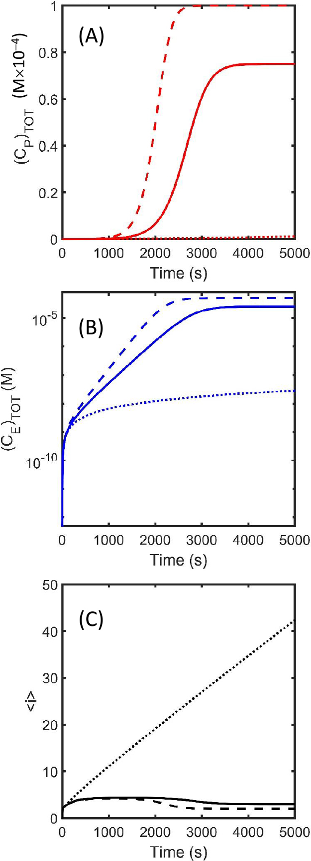
Effect on amyloid growth rate due to differences in internal (b_S2) and end (b_S1) breakage rates: Amyloid formation kinetics are simulated via numerical integration of Eq. 4 and 5 (utilizing the approximations derived in Eq. 6 and 7) for three relative cases reflecting a different ratio, θ, of the internal to end breakage rates such that θ=b_S2/b_S1. The simulations were carried out for a system where fiber joining does not occur using the following common values for additional parameter values, f_N=0.001 M^–1s^–1, f_G=200 M^–1s^–1, f_J=0 M^–1s^–1 and (C₁)_TOT=0.1 mM. The figure panels describe the formation of (A) (C_P)_TOT, (B) (C_E)_TOT and (C) $⟨i⟩$. The three different cases corresponding to differences in internal versus end breakage rates are specified as followed—solid lines (–) θ=1 (b_S1=b_S2=0.0025 s^–1); dashed lines (- -) θ→∞ (b_S1=0 s^–1, b_S2=0.0025 s^–1); dotted lines (···) θ=0 (b_S1=0.0025 s^–1s^–1, b_S2=0 s^–1).

Results and Discussion

The described approach provides an extraordinarily simple means for incorporating differential fiber breakage susceptibilities occurring either internally, thereby creating two new fibers, or at the fiber ends, thereby releasing a monomer unable to maintain the amyloid structure. From Figure 2 we note that as θ increases from zero, the rate of total amyloid formation, $\frac{d{\left(C_P\right)}_{\mathrm{T}\mathrm{O}\mathrm{T}}}{dt}$, increases (Fig. 2a) as a result of an increased rate of production of fiber ends, $\frac{d{\left(C_E\right)}_{\mathrm{T}\mathrm{O}\mathrm{T}}}{dt}$ (Fig. 2b), with a necessarily concomitant decrease in the average amyloid degree, $⟨i⟩$ (Fig. 2c). As discussed previously [9,19] and again more recently in Nicoud, L., et al. [16], such position dependent breakage suscepti­bilities may produce dramatic consequences for the development of biological or pharmaceutical agents designed to either promote fiber dissolution [20,21] or fiber stabilization [21]. Deeper appreciation of this point can be gotten when interpreting the situation through the lens of the fiber breakage model of amyloidosis disease advanced by Hall and Edskes [19,22].

Although simulation results are dependent upon the values of the parameters adopted, confidence can be placed in the general trends shown in Figure 2 for the following three reasons. (i) Chosen parameters conform to a kinetically nucleated system (i.e. f_G>>f_N) thereby producing the classical sigmoidal kinetic curve that is a characteristic hallmark of amyloid growth [3–10]. (ii) Adopted parameters describe a thermodynamically nucleated system (helical polymerization) in which the total monomer concentration is much greater than the characteristic critical concentration i.e. (C₁)_TOT>>b_S1/f_G (when b_S2=0) or (C₁)_TOT>>b_S2/f_G (when b_S1=0) [1–4,19,21]. (iii) Simulations transition from one extreme limiting case of relative breakage to the other i.e. θ is examined over the range [0, ∞). In the present instance although different parameters will change absolute behavior (i.e. different time scale and extents) they will not change the relative behavior—the exposition of which is the chief interest in this Note.

The principle assumption within the paper involves the method for estimation of C₂. To gain an appreciation as to why the adopted approach is valid we first note that the amyloid kinetic model is founded in the numerical integration of just two differential equations (Eq. 4 and 5) with the dependent variables describing the concentration of amyloid ends, (C_E)_TOT, and total monomer in amyloid, (C_P)_TOT (Eq.1 and 2). Due to its presence as a vanishing term in Eq. 4 and 5, error in the estimation of C₂ will be virtually insignificant as the polymer distribution increases in size (i.e. C₂/(C_E)_TOT→0; 2C₂/(C_P)_TOT→0) thereby making the need for its accurate evaluation under these conditions unimportant [14,23]. At the other extreme, when C₂ constitutes all of the amyloid fiber (i.e. C₂/(C_E)_TOT=1; 2C₂/(C_P)_TOT=1), its evaluation is exact (see Appendix 2). Within the intermediate region (as these fractions decrease from 1) the exponential assumption will essentially be a linear approximation, especially so for low average degree of polymerization e.g. [2 < $⟨i⟩$ < 2.5]. Beyond the initial intermediate region (as $⟨i⟩$ > 2.5) the correctness of the exponential distribution assumption will become less exact but not dramatically so, as due to its physical origin (as the result of a sequential indefinite polymerization reaction) the amyloid fiber number concentration distribution will be exponential in character, especially at early times when (C_P)_TOT is increasing [23,24]. As such, the simple model described in the present paper will be sufficient to assist with (i) simulation of the early time course of amyloid formation featuring differential fiber breakage related to position of the bond within the fiber, and (ii) characterization of experimental kinetics via its use in non-linear regression based fitting analysis. (Note—By early time course I am referring to the vastly different time scales in fiber polymerization identified for attainment of (i) the monomer/polymer mass pseudo-equilibrium, and (ii) the polymer length distribution [19,24,25]. The assumption of an exponential distribution is expected to be less correct for prediction of this second ‘later’ time scale than for prediction of the first ‘early’ time scale).

Two other notable assumptions made within the present work are (i) the use of a phenomenological nucleus of a size set at two monomers, and (ii) set equivalence of the nucleus dissociation rate and terminal monomer dissociation rate from the amyloid fibril. The first of these additional assumptions was made due to concerns based on partly practical and partly scientific reasons. The practical concerns are due to vagaries associated with classification of aggregate identity. If the nucleus size were to be appreciable (say 10 monomers) and formed in a stepwise fashion, then aggregate species between size 2 and 10 may be either amyloid or non-amyloid pre-nucleus in character. Determination of the nature of these species is experimentally difficult and further complicated by distinguishing whether or not they are associated with on, off or parallel pathways [14,26,27]. Scientific concerns relate to the way the nucleus size has been previously asserted via model based kinetic fitting. Results shown in Figure 2a clearly belie (or at least should raise a warning flag) any estimate of nucleus size based on use of fitting models featuring uniform breakage rates or size-independent growth rates [16,19,28]. As such, I would suggest that a minimal assumption of a nucleus size of 2 is suitable for the development of the current low parameter minimal model. Justification for the second of these additional assumptions (an assumed common rate of monomer dissociation from amyloid and nucleus i.e. both characterized by b_S1) is harder to provide due to the fact that such information could only be supplied by isolated time-dependent observations made at the nanometer level of resolution (at present impossible). However, following an Occam’s razor type argument (in which models involving less parameters have greater scientific utility until proven inadequate) a judgement on this question should only be made on the basis of data analysis—for which no such suitable data currently exist.

Conclusions

Due to the fact that the method developed here does not describe an exact geometric dependence the current approach is likely applicable to the description of other systems involving one, two and three-dimensional polymerization processes. Like the model introduced by Smith, J. F., et al. [15] the current set of equations are simple enough that it can be easily incorporated into more complex simulation routines describing amyloidosis disease models [19,29,30], complex mixture models [14,26,31], signal identification and processing [13,27,32–34], polymer statistics based approaches involving amyloid formation from the unfolded protein state [8,28,35], or in ‘meta-models’ describing the transmission of prions in larger scale, more complex studies, involving organism level analysis of yeast, worms and flies [36–38]. Indeed use of Eq. 2 may help to cast light on the molecular mechanisms of candidates identified in ‘Anti-Prion’ screens [39].

Acknowledgements

I would like to thank (the now) Dr. Jeffrey Smith for a number of interesting discussions related to the present topic conducted during the course of his (JS’s) PhD. I acknowledge thoughtful comments from the two Reviewers who provided an exceptionally high quality review of the manuscript. I thank Dr. H.K. Edskes for helpful discussion and a highly enjoyable 15 years of collaborative work. I thank the Institute for Protein Research at Osaka University for the support they have provided over the last 5 years. I gratefully acknowledge the US Government for funds provided in the form of an ORISE Established Scientist Position. This research was supported in part by an appointment to the National Library of Medicine (NLM) Research Participation Program. This program is administered by the Oak Ridge Institute for Science and Education through an interagency agreement between the U.S. Department of Energy (DOE) and the National Library of Medicine (NLM). ORISE is managed by ORAU under DOE contract number DE-SC0014664. All opinions expressed in this paper are the author’s and do not necessarily reflect the policies and views of NLM, DOE, or ORAU/ORISE.

Conflicts of Interest

The author declares no conflict of interest.

Author Contribution

D.H. developed the theory and wrote the manuscript.

References

• [1]   Oosawa,  F. &  Kasai,  M. A theory of linear and helical aggregations of macromolecules. J. Mol. Biol. 4, 10–21 (1962). DOI: 10.1016/S0022-2836(62)80112-0
• [2]  Oosawa, F. & Asakura, S. Thermodynamics of the Polymerization of Protein (Academic Press, New York, 1975).
• [3]   Naiki,  H.,  Higuchi,  K.,  Nakakuki,  K. &  Takeda,  T. Kinetic analysis of amyloid fibril polymerization in vitro. Lab. Invest. J. Tech. Meth. Path. 65, 104–110 (1991).
• [4]   Naiki,  H.,  Hashimoto,  N.,  Suzuki,  S.,  Kimura,  H.,  Nakakuki,  K. &  Gejyo,  F. Establishment of a kinetic model of dialysis-related amyloid fibril extension in vitro. Amyloid 4, 223–232 (1997). DOI: 10.3109/13506129709003833
• [5]   Khan,  M. A.,  Islam,  M. M. &  Kuroda,  Y. Analysis of protein aggregation kinetics using short amino acid peptide tags. Biochim. Biophys. Acta Proteins Proteom. 1834, 2107–2115 (2013). DOI: 10.1016/j.bbapap.2013.06.013
• [6]   Kuroda,  Y. Biophysical studies of protein solubility and amorphous aggregation by systematic mutational analysis and a helical polymerization model. Biophys. Rev. 10, 473–480 (2018). DOI: 10.1007/s12551-017-0342-y
• [7]   Masel,  J.,  Jansen,  V. A. &  Nowak,  M. A. Quantifying the kinetic parameters of prion replication. Biophys. Chem. 77, 139–152 (1999). DOI: 10.1016/s0301-4622(99)00016-2
• [8]   Pallitto,  M. M. &  Murphy,  R. M. A mathematical model of the kinetics of β-amyloid fibril growth from the denatured state. Biophys. J. 81, 1805–1822 (2001). DOI: 10.1016/S0006-3495(01)75831-6
• [9]   Hall,  D. &  Edskes,  H. Silent prions lying in wait: a two-hit model of prion/amyloid formation and infection. J. Mol. Biol. 336, 775–786 (2004). DOI: 10.1016/j.jmb.2003.12.004
• [10]   Binger,  K. J.,  Pham,  C. L.,  Wilson,  L. M.,  Bailey,  M. F.,  Lawrence,  L. J.,  Schuck,  P., et al. Apolipoprotein C-II amyloid fibrils assemble via a reversible pathway that includes fibril breaking and rejoining. J. Mol. Biol. 376, 1116–1129 (2008). DOI: 10.1016/j.jmb.2007.12.055
• [11]   Andrews,  J. M. &  Roberts,  C. J. A Lumry− Eyring nucleated polymerization model of protein aggregation kinetics: 1. Aggregation with pre-equilibrated unfolding. J. Phys. Chem. B 111, 7897–7913 (2007). DOI: 10.1021/jp070212j
• [12]   Kashchiev,  D. Protein polymerization into fibrils from the viewpoint of nucleation theory. Biophys. J. 109, 2126–2136 (2015). DOI: 10.1016/j.bpj.2015.10.010
• [13]   Zhao,  R.,  So,  M.,  Maat,  H.,  Ray,  N.,  Arisaka,  F.,  Goto,  Y., et al. Measurement of amyloid formation by turbidity assay—seeing through the cloud. Biophys. Rev. 8, 445–471 (2016). DOI: 10.1007/s12551-016-0233-7
• [14]   Hirota,  N.,  Edskes,  H. &  Hall,  D. Unified theoretical description of the kinetics of protein aggregation. Biophys. Rev. 11, 191–208 (2019). DOI: 10.1007/s12551-019-00506-5
• [15]   Smith,  J. F.,  Knowles,  T. P.,  Dobson,  C. M.,  MacPhee,  C. E. &  Welland,  M. E. Characterization of the nanoscale properties of individual amyloid fibrils. Proc. Nat. Acad. Sci. USA 103, 15806–15811 (2006). DOI: 10.1073/pnas.0604035103
• [16]   Nicoud,  L.,  Lazzari,  S.,  Barragán,  D. D. &  Morbidelli,  M. Fragmentation of amyloid fibrils occurs in preferential positions depending on the environmental conditions. J. Phys. Chem. B 119, 4644–4652 (2015). DOI: 10.1021/acs.jpcb.5b01160
• [17]   Han,  W. &  Schulten,  K. Fibril elongation by Aβ(17–42): kinetic network analysis of hybrid-resolution molecular dynamics simulations. J. Am. Chem. Soc. 136, 12450–12460 (2014). DOI: 10.1021/ja507002p
• [18]   Heldt,  C. L.,  Zhang,  S. &  Belfort,  G. Asymmetric amyloid fibril elongation: A new perspective on a symmetric world. Proteins 79, 92–98 (2011). DOI: 10.1002/prot.22861
• [19]   Hall,  D. &  Edskes,  H. A model of amyloid’s role in disease based on fibril fracture. Biophys. Chem. 145, 17–28 (2009). DOI: 10.1016/j.bpc.2009.08.004
• [20]   Doig,  A. J.,  del Castillo-Frias,  M. P.,  Berthoumieu,  O.,  Tarus,  B.,  Nasica-Labouze,  J.,  Sterpone,  F., et al. Why is research on amyloid-β failing to give new drugs for Alzheimer’s disease? ACS Chem. Neurosci. 8, 1435–1437 (2017). DOI: 10.1021/acschemneuro.7b00188
• [21]   Panza,  F.,  Seripa,  D.,  Solfrizzi,  V.,  Imbimbo,  B. P.,  Lozupone,  M.,  Leo,  A., et al. Emerging drugs to reduce abnormal β-amyloid protein in Alzheimer’s disease patients. Expert. Opin. Emerg. Drugs 21, 377–391 (2016). DOI: 10.1080/14728214.2016.1241232
• [22]   Hall,  D. &  Edskes,  H. Computational modeling of the relationship between amyloid and disease. Biophys. Rev. 4, 205–222 (2012). DOI: 10.1007/s12551-012-0091-x
• [23]  Elimelech, M., Gregory, J., Jia, X. & Williams, R. A. in Particle Deposition & Aggregation: Measurement, Modelling and Simulation (Williams, R. A. ed.) Colloid and Surface Engineering, Chapter 6 Modelling of Aggregation Processes (Butterworth-Heinemann, 1998).
• [24]   Hall,  D. &  Minton,  A. P. Effects of inert volume-excluding macromolecules on protein fiber formation. (II.) Kinetic models for nucleated fiber growth. Biophys. Chem. 107, 299–316 (2004). DOI: 10.1016/j.bpc.2003.09.016
• [25]   Hall,  D. The effects of denaturation of tubulin on the characterization of its polymerization behavior. Biophys. Chem. 104, 655–682 (2003). DOI: 10.1016/s0301-4622(03)00040-1
• [26]   Hall,  D.,  Kardos,  J.,  Edskes,  H.,  Carver,  J. A. &  Goto,  Y. A Multi-Pathway Perspective on Protein Aggregation: Implications for the Rate and Extent of Amyloid Formation. FEBS Lett. 589, 672–679 (2015). DOI: 10.1016/j.febslet.2015.​01.032
• [27]   Hall,  D.,  Zhao,  R.,  Dehlsen,  I.,  Bloomfield,  N.,  Williams,  S. R.,  Arisaka,  F., et al. Protein aggregate turbidity: Simulation of turbidity profiles for mixed-aggregation reactions. Anal. Biochem. 498, 78–94 (2016). DOI: 10.1016/j.ab.​2015.11.021
• [28]   Hall,  D. &  Hirota,  N. Multi-scale modelling of amyloid formation from unfolded proteins using a set of theory derived rate constants. Biophys. Chem. 140, 122–128 (2009). DOI: 10.1016/j.bpc.2008.11.013
• [29]   Craft,  D. L.,  Wein,  L. M. &  Selkoe,  D .J. A Mathematical Model of the Impact of Novel Treatments on the Aβ-Burden in the Alzheimer’s Brain, CSF and Plasma. Bull. Math. Biol. 64, 1011–1031 (2002). DOI: 10.1006/bulm.2002.0304
• [30]  Weickenmeier, J., Kuhl, E. & Goriely, A. Multiphysics of prionlike diseases: Progression and atrophy. Phys. Rev. Lett. 121, 158101-1–158101-6 (2018). DOI: 10.1103/PhysRevLett.​121.158101
• [31]   Nitani,  A.,  Muta,  H.,  Adachi,  M.,  So,  M.,  Sasahara,  K.,  Sakurai,  K., et al. Heparin-dependent aggregation of hen egg white lysozyme reveals two distinct mechanisms of amyloid fibrillation. J. Biol. Chem. 292, 21219–21230 (2017). DOI: 10.1074/jbc.M117.813097
• [32]   Hall,  D. &  Huang,  L. On the use of size-exclusion chromatography for the resolution of mixed amyloid aggregate distributions (I) Equilibrium partition models. Anal. Biochem. 426, 69–85 (2012). DOI: 10.1016/j.ab.2012.04.001
• [33]   Hall,  D. Semi-automated methods for simulation and measurement of amyloid fiber distributions obtained from transmission electron microscopy experiments. Anal. Biochem. 421, 262–277 (2012). DOI: 10.1016/j.ab.2011.10.012
• [34]   Hall,  D.,  Zhao,  R.,  So,  M.,  Adachi,  M.,  Rivas,  G.,  Carver,  J. A., et al. Recognizing and analyzing variability in amyloid formation kinetics. Anal. Biochem. 510, 56–71 (2016). DOI: 10.1016/j.ab.2016.07.013
• [35]   Hall,  D.,  Kinjo,  A. R. &  Goto,  Y. A new look at an old view of denaturant induced protein unfolding. Anal. Biochem. 542, 40–57 (2018). DOI: 10.1016/j.ab.2017.11.011
• [36]   Tanaka,  M.,  Collins,  S. R.,  Toyama,  B. H. &  Weissman,  J. S. The physical basis of how prion conformations determine strain phenotypes. Nature 442, 585–589 (2006). DOI: 10.1038/nature04922
• [37]   Bieschke,  J.,  Cohen,  E.,  Murray,  A.,  Dillin,  A. &  Kelly,  J. W. A kinetic assessment of the C. elegans amyloid disaggregation activity enables uncoupling of disassembly and proteolysis. Protein Sci. 18, 2231–2241 (2009). DOI: 10.1002/pro.234
• [38]   Pokrzywa,  M.,  Pawełek,  K.,  Kucia,  W. E.,  Sarbak,  S.,  Chorell,  E., Almqvist,  F., et al. Effects of small-molecule amyloid modulators on a Drosophila model of Parkinson’s disease. PLoS ONE 12, e0184117 (2017). DOI: 10.1371/journal.pone.0184117
• [39]   Wickner,  R. B.,  Son,  M. &  Edskes,  H. K. Prion Variants of Yeast are Numerous, Mutable, and Segregate on Growth, Affecting Prion Pathogenesis, Transmission Barriers, and Sensitivity to Anti-Prion Systems. Viruses 11, 238 (2019). DOI: 10.3390/v11030238

Appendix

Appendix 1: Complete derivation of Eq. 4 and 5

To derive Eq. 4 we begin by writing out the rate equation that corresponds to the actual set of allowable elementary steps.

  

$$\begin{array}{cc}\frac{d{\left(C_E\right)}_{TOT}}{dt}=\hfill & f_N{C}_1^2+\sum _{i=4}^z{b}_{S2}{C}_i(i-3)-b_{S1}{C}_2\\ & -f_J\sum _{m=2}^z{C}_m\sum _{n=2}^z{C}_n\hfill \end{array}$$(A1)

By noting (i) when i=2, b_S2 C₂+b_S2 C_i(i–3)=0, and (ii) when i=3, b_S2 C_i(i–3)=0, we can rewrite Eq. A1 as A2.

  

$$\begin{array}{cc}\frac{d{\left(C_E\right)}_{TOT}}{dt}=\hfill & f_N{C}_1^2+\sum _{i=2}^z{b}_{S2}{C}_i(i-3)+b_{S2} C_2\hfill \\ & -b_{S1}{C}_2-f_J{{\left(C_E\right)}_{TOT}}^2\hfill \end{array}$$(A2)

Based on Eq. 1 and 2 we can rewrite Eq. A2 as Eq. 4.

With regard to Eq. 5 we similarly begin by writing out rate equation from allowable elementary steps (Eq. A3).

  

$$\frac{d{\left(C_P\right)}_{TOT}}{dt}=2f_N{C}_1^2-2b_{S1}\sum _{i=2}^z{C}_i+f_G\left(\sum _{i=2}^z{C}_i\right)C_1^{}$$(A3)

Substitution of the identities shown in Eq. 1 allow Eq. A3 to be re-expressed as Eq. 5.

Appendix 2: Derivation of an analytical approximant for C₂

To obtain Eq. 7 we approximate the two discrete summations in the left-hand side of Eq. A4 with two separate integrals.

  

$$⟨i⟩=\frac{{\sum }_{i=2}^z\mathrm{i}.e^{\left(-k.i\right)}}{{\sum }_{i=2}^z{e}^{\left(-k.i\right)}}\approx \mathrm{ }\frac{{\int }_{i=2}^{i=\infty }i.e^{\left(-k.i\right)}di}{{\int }_{i=2}^{i=\infty }{e}^{\left(-k.i\right)}di} = 2+\mathrm{ }\frac{1}{{ }^k}$$(A4)

With the value of $⟨i⟩$ determined at each step of the numerical integration cycle by Eq. 3 a value for k can be determined by solving Eq. 7 for the case of $⟨i⟩$ > 2 and then substituting this value for k into Eq. 6 solving for i = 2. For the case of $⟨i⟩$ = 2 we set C₂ = (C_E)_TOT.