Special Issue: The Oosawa Lectures on DIY Statistical Mechanics
Chapter 3: Changing the Rules
2021 年 18 巻 Supplemental 号 p. S025-S034
詳細
2021 年 18 巻 Supplemental 号 p. S025-S034
In the previous chapter, the rule was that if a person with 0 gaming chips was hit, the number of trials were incremented without debt. An interesting variation of this rule involves elimination of the player via inclusion of the concept of bankruptcy from society, i.e., a person with 0 gaming chips is eliminated from the game (Fig. 3.1)3.1. In this case, since the total number of gaming chips will be the same, however, the number of players will decrease, therefore the average number of gaming chips per person will increase. Nevertheless, the number of bankruptcies (persons with 0 gaming chips) will continue to increase, as such persons appear every moment (Fig. 3.1; Bar at the left end of the figure on the right). If we keep it going, only a small number of rich people will survive.

Bankruptcy elimination. Before exchange (A), after 5,000 exchanges (B), and after 50,000 exchanges (C). The horizontal axis of the left figures represents player indices (100 players in total) and the vertical axis represents the number of gaming chips each one has. Figures on the right-hand side show the histogram of the gaming chip distribution with the number of gaming chips shown on the (horizontal axis) with the number of players having a certain number of gaming chips shown on the (vertical axis) at each time point. The rules are as follows:
· 20,000 chips in 100 boxes
· Persons with 0 chips are eliminated (bankruptcy elimination)
· The dice roll hits equally with respect to the box (consumption tax type)
If you wonder whether this is just a demonstration, the answer is NO. I apologize for suddenly jumping to another topic, however, there is an experiment called the G-F conversion of F-actin3.2 about which a mild diversion into discussion will prove particularly instructive [3.1–3.3]. The fact revealed in the prior chapter, that the distribution in the chip exchange game eventually relaxes into an exponential distribution (geometric series) from its starting state resembling a normal distribution, is to me, the very story of the actin polymerization experiment. Actin is a discrete monomeric protein that is able to polymerize i.e. join together in a regular manner to form a linear protein fiber. At the outset of this joining process, many nuclei (seeds) are formed3.3. Due to their generally small and ubiquitous nature these nuclei are approximately uniformly distributed. Most of these nuclei continue to grow longer and longer at a similar rate. Monomers are continuously withdrawn from the supersaturated liquid due to their chemical attraction to the seeds, and therefore the polymer continues to tend to grow uniformly. Hence, the initial result is a sharply configured normal distribution with fibers of almost the same length (Fig. 3.2A)3.4. However, over a much longer time the monomeric G-actin and the polymeric F-actin reach equilibrium, and when they reach the G-F equilibrium, the exchange probabilities become equal (Fig. 3.2) and the size distribution transforms into an exponential (geometric series) distribution (Fig. 3.2B) [3.4].

Actin polymerization. Schematic diagram of a linear polymer (crystal) growth by polymerization of monomers (white circles) to the nuclei (represented with two black circles) (Left), and length distribution (Right: Histogram showing the horizontal axis is the length of the polymer and the vertical axis is the number of polymers of that length). A: In the initial stage of the reaction, there are excess monomers and the polymer grows rapidly. At this time, since there are excess monomers, the polymerization (left arrow) reaction is dominant in comparison to dissociation of the monomer from the fiber (right arrow). This corresponds to the initially distributed state before exchange in the dice and chip game. B: As the reaction proceeds, the number of monomers decreases, and the rate of polymerization (left arrow) and depolymerization (right arrow) reactions become balanced. This situation directly corresponds to the state of exchange in the dice and chip game.
What I have just described is what really happens in such an actin G/F transition experiment, and it was quite an interesting story at the time of its first discovery [3.5]. Theoretical analysis has allowed kinetic equations for polymer-growth to be written. The initial distribution of fiber length predicted by such theoretical models is indeed a normal distribution. However, after waiting for sufficient time to reach equilibrium, the distribution will become exponential. In addition, the time until it becomes an exponential distribution can be calculated. Since it is the same as the diffusion process (the process of Brownian motion, Chapter 8), the time is proportional to the square of the number of monomers within the fiber, that is, to the square of the length. In the actual experiment, it initially took approximately an hour to grow. However, it took one day to obtain the exponential distribution (geometric series distribution).
It was also determined that the same growth rate equation can be applied to three-dimensional protein crystals. Because F-actin only grows linearly, it seems strange how the same theoretical equations developed to describe its growth can be applied just as successfully to the description of 3D crystals3.5. Perhaps, even 3D crystals have one growth point. In other words, since they elongate in a helical fashion, they must grow linearly. This supposition turns out to be true and therefore the equations used for linear growth can indeed be successfully applied to crystal formation. A research group showed that lysozyme crystals exhibit the same type of growth behavior [3.6]3.6. In the case of protein crystals, at the beginning, the seeds start and grow uniformly. Then, as the exchange process starts, the crystal sizes become non-uniform in size. When the rate of crystallization of the dissolving solute and the rate of dissolution of the solute from the crystal reach equilibrium, such that larger and smaller crystals gradually appear. If the smaller crystals are reduced to zero, they cannot reappear. Hence, it is exactly the theory of bankruptcy elimination, whereby if you wait patiently, one large crystal will eventually be formed. The group has been experimenting for one year, so their experiment is amazing. However, fast growth advances in the order of seconds.
The prior discussion shows why the current topic is both interesting while also being very practical in its application to both economics and biophysics. In the case of bankruptcy elimination, simulations show the process of how distributions of large crystals can emerge from the normal to exponential (geometric series) distribution transition (potentially resulting in just one crystal). Now, compare Fig. 2.6 and Fig. 3.1 again. Fig. 2.6 shows the case with bankruptcy survival. We started a one-to-one exchange with 100 players and a total of 2,000 gaming chips. After the preceding discussion you will now be able to appreciate the nature of the change in distribution. Fig. 3.1 shows the case with the bankruptcy elimination. Bankruptcies increase and players disappear. Indeed, after a sufficient number of exchanges, there will be just one individual remaining. It’s quite amazing, isn’t it? It is quite interesting how many noteworthy experimental facts can emerge when we play a simple dice and chip game!
Until now, the gaming chips were exchanged with equal probability regardless of the number of gaming chips one possesses. In the following, we will examine the case whereby the probability of exchange depends on the number of gaming chips one possesses.
Considering the case of only two people exchanging gaming chips, first we divide the total of 30 gaming chips into 15 each, and then we start the exchange. We compare two cases, the first of which corresponds to the situation whereby the exchange is performed as before (an equal probability per person) and a second, in which the probability of giving out gaming chips is proportional to the number of gaming chips one possesses, i.e. if more money is held the probability of giving the gaming chip is greater (an equal probability per gaming chip). Since the case of two individuals is the most extreme and easy to understand, the results calculated by computer for both cases are shown in Fig. 3.3. In the case of giving out gaming chips in proportion to the number of gaming chips a person possesses (income tax-type, black line in Fig. 3.3, case2), we see that the number of gaming chips fluctuates around 15. If exchange is performed with an equal probability per person (gray in Fig. 3.3, case1), exchange will be finished quickly with the eventual bankrupt of one of the two people. When exchange is performed with an equal probability per gaming chip, there is a restoring force to the center, and as a result the distribution of chips will fluctuate around the center, similar to a normal distribution (Table 3.1)3.7.

Consumption tax type and the income tax type. Comparison of the consumption tax type (case 1 where there is no restoring force – gray line) and the income tax type (case 2 where there is a restoring force – black line). Two individuals exchange 30 chips in total. The vertical axis is the number of gaming chips held by one of the two people and the horizontal axis is the number of trials. In case 1, the exchange ends after the 80th trial when one of the two participants becomes bankrupt i.e. they have zero chips.
| The difference between the two cases will be evident by playing the game with two people. | |
| Case1: Consumption tax type | |
| Rule: | Fairness to the box (person) (does not depend on the number of gaming chips in the box) |
| Result: | Either one will be zero (Fig. 3.3 gray) |
| Case2: Income tax-type | |
| Rule: | Fairness to the gaming chips (no matter in which box (person) the coins be) |
| Result: | Both chips will return to equal because of restoring force (Fig. 3.3 black). |
Please investigate what will happen if we play with an equal probability per gaming chip (income tax rule), for the case of 3 gaming chips distributed amongst 3 persons listed as A, B and C (Exercise 3). What is the probability of going from (3, 0, 0) to (2, 1, 0)? Try drawing a diagram with arrows used to represent the exchange. For various ways of rolling the dice, please write as many arrows as there are possible transitions between the states. As an example, in determining the probability of going from the (2, 1, 0) state to the (3, 0, 0) state, the probability for the one gaming chip that B holds is just 1, so as a result we just draw one arrow. When going from (3, 0, 0) to (2, 1, 0), since it can be any one of the 3 gaming chips that A holds, we draw 3 arrows. In this way, by drawing arrows, you will be able to understand just how many equivalent ways the process can occur.
In Exercise 2, we played using the rule whereby gaming chips were given with an equal probability per person. Here, we consider the case of giving gaming chips with an equal probability per gaming chip held by the player. Three persons (A, B, and C) exchange 3 gaming chips.
1. Write arrows corresponding to all the paths for exchange between the states in Fig. 3.4. Unlike Exercise 2, the number of arrows that originate from each state is equal to the number of gaming chips in the original state. For example, there are three equivalent arrows for each of the transitions from (3, 0, 0) to (2, 1, 0) and (2, 0, 1). On the contrary, only one arrow is used to describe the reverse transition from (2, 1, 0) and (2, 0, 1) to (3, 0, 0). A person with 0 gaming chips will have an exchange probability of 0, i.e. the rule is that debt is not allowed.
2. Determine the probability of all the states. Set the probability of A having all 3 gaming chips P(3, 0, 0)=p, the probability of A having 2 gaming chips and B having 1 gaming chip as P(2, 1, 0)=q, and the probability of each person having 1 gaming chip as P(1, 1, 1)=r. The probabilities of all the other 7 states can be represented using p, q, r. The probability (r) of becoming (1, 1, 1) is described as the probability of transition from the surrounding 6 states (q) with a probability of 1/6. In the same way, determine the values of p, q, and r.
3. Determine the probabilities about C with 0, 1, 2, and 3 gaming chips, respectively.
(See Fig. 3.5 for the answers.)

Exercise 3. Diagram of all the cases of distribution of three chips amongst three persons A, B, and C. All the possible transitions are indicated by the dashed lines. Please fill out their probabilities.
From Exercise 3, the ratio of the probabilities of the respective final states of (3, 0, 0) and (2, 1, 0) and so on can be determined. In the case of exchange with an equal probability per person (case 1), it was 4, 3, 2, 1 for 0, 1, 2, 3 respectively. However, this time, in the income tax-type (case 2), the frequency (probability) is maximized at one gaming chip but not at zero chips, as in case 2 (Fig. 3.5). I would appreciate it if you could try it out for yourself and see how different it is. Although you have already understood the theory, my objective is to allow you to gain experience by investigating very simple cases through practical experimentation via the drawing of arrows.

All methods of distributing 3 chips to 3 boxes, with equal probability per chip. The number of arrows indicates the probability and the direction of change due to the exchange (Answers to Exercise 3).
As shown in Fig. 3.6, if the exchanges are made with an equal probability per person (case1), the frequency decreases in the same order as 0, 1, 2, 3 gaming chips, whereas, if the exchanges are made with an equal probability per gaming chip (case 2), there is a peak in the middle aside from 0 gaming chips. This can be understood by drawing arrows as shown (Fig. 3.5). You may understand this by writing down the diagram describing what happens when there are 3 gaming chips distributed amongst 3 persons, and that there are remarkable differences between the cases reflecting exchange conducted on a per person (case 1) and per gaming chip (case 2) basis. Fig. 3.6 illustrates this symbolically. What I mean is that even with such a small number of persons and gaming chips, you can appreciate these differences manually. If you experiment, you will understand.
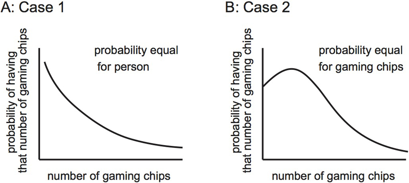
Difference in exchange reflecting probability per person and probability per chip held. Comparison of the distribution of the number of gaming chips per person between cases where the probability of giving a gaming chip is equal per person (case 1), and the case when it is equal per number of chips (case 2). The horizontal axis is the number of chips held per person and the vertical axis is the probability of having that number of gaming chips.
So far, we have focused on counting the states in just one box. However, what if we focus on counting states in two boxes? Stated in such a way this seems a simple question but it is, in fact, the key point of statistical mechanics. A simple extension would be to consider two boxes out of a total of five boxes. Again, I would like the reader to investigate this situation through drawing the states by hand (Exercise 4).
Determine the total number of ways that chips can be distributed, focusing on the first two boxes (Table 3.2).
1. Write down the ways that a total of 0 to 5 gaming chips can be distributed between the first two boxes (A, B), and then how the remaining 5 to 0 gaming chips can be distributed amongst the remaining three boxes (C, D, E). Determine the total number of distinct states (the total number of ways) of arranging each case. The number of gaming chips in 3 boxes can be written in a horizontal row as a three-digit number, and this number is written in ascending order. For the case of 3 gaming chips in 3 boxes, it is 003, 012, 021, 030, 102, 120, 111, 201, 210, and 300. Similarly, the number of ways of arranging 2 chips in 2 boxes can be written as (20,11,02).
2. What is the total number of ways of distributing 5 gaming chips in 5 boxes? Determine by calculation and not by writing.
Idea: The total number of ways of arranging two separate cases can be calculated as the product of the number of cases of arranging each separate case i.e. Total Cases=Cases (A, B)×Cases (C, D, E)
| The two considered boxes [A, B] |
Remaining three boxes [C, D, E] |
Number of cases of 5 boxes |
||||
|---|---|---|---|---|---|---|
| Number of gaming chips |
Distribution method | Number of cases |
Number of gaming chips |
Distribution method | Number of cases |
Number of cases |
| 0 | 5 | |||||
| 1 | 4 | |||||
| 2 | 3 | |||||
| 3 | 2 | |||||
| 4 | 1 | |||||
| 5 | 0 | |||||
| The two considered boxes [A, B] |
Remaining three boxes [C, D, E] |
Number of cases 5 boxes |
||||
|---|---|---|---|---|---|---|
| Number of gaming chips |
Distribution method | Number of cases |
Number of gaming chips |
Distribution method | Number of cases |
Number of cases |
| 0 | 00 | 1 | 5 | 005, 014, 023, 032, 041, 050, 104, 113, 122, 131, 140, 203, 212, 221, 230, 302, 311, 320, 401, 410, 500 | 21 | 21 |
| 1 | 01, 10 | 2 | 4 | 004, 013, 022, 031, 040, 103, 112, 121, 130, 202, 211, 220, 301, 310, 400 | 15 | 30 |
| 2 | 02, 11, 20 | 3 | 3 | 003, 012, 021, 030, 102, 120, 111, 201, 210, 300 | 10 | 30 |
| 3 | 03, 12, 21, 30 | 4 | 2 | 002, 011, 020, 101, 110, 200 | 6 | 24 |
| 4 | 04, 13, 22, 31, 40 | 5 | 1 | 001, 010, 100 | 3 | 15 |
| 5 | 05, 14, 23, 32, 41, 50 | 6 | 0 | 000 | 1 | 6 |
In this discussion, we place our focus on two boxes (A, B) out of five boxes (A, B, C, D, E) in total amongst which five gaming chips are distributed. We now attempt to provide an example initially by just counting the number of cases of storing gaming chips in the first two boxes (A, B) (Exercise 4). As an example, we respectively define the number of cases of distributing 0, 1, 2 or 3 chips amongst these two (A, B) boxes as (0, 0) for a total of 0 gaming chips in 2 boxes, (0, 1) and (1, 0) for a total of 1 chip, (2, 0), (1, 1), and (0, 2) for a total of 2 gaming chips, and (3, 0), (2, 1), (1, 2), and (0, 3) for a total of 3 gaming chips. At this time, please examine the states defined in Table 3.3 and Fig. 3.7 for storing a total number of 0, 1, 2 and 3 gaming chips in these two boxes. Indeed, we see that the numbers of ways are 1, 2, 3, and 4 respectively, which means that when the total number of gaming chips increases by 1, the number of ways of storing these chips increases by 1 (Fig. 3.7B black line). However, as we put more of the chips into the first two boxes the number of ways of distributing the leftover gaming chips in the remaining 3 boxes decreases in a nearly geometric series (Fig. 3.7B gray line). As the total number of chips in the two boxes increases from 0, 1, 2, … the number of cases initially doubles from 1 to 2 ways, and then increases 1.5 times from 2 to 3 ways. Note that although the absolute number of cases increases, the ratio between consecutive cases actually decreases. Thus, if we increase the number of considered boxes from 1 to 2 (or more), a peak in the number of cases will be created.

A: All the ways of distributing 5 chips in 5 boxes. When we consider 2 different groups of boxes. B: The horizontal axis is the total number of gaming chips in the first two boxes, and the vertical axis is the count of the possible number of cases for arranging that number of gaming chips.
Fig. 3.8A shows the case of 6 gaming chips in 6 boxes (N=6, M=6) and Fig. 3.8B shows the case of 24 gaming chips in 6 boxes (N=24, M=6). Please note that the figure has a peak in the middle. Thus, when the considered boxes are changed from 1 to 2, a peak will certainly appear. Fig. 3.8C shows the results of rolling the dice by hand. The figure shows the results for 18 and 36 gaming chips in 6 boxes (N=18; 36, M=6).

Case of distributing gaming chips within the first 2 considered boxes [A, B] out of 6 boxes [A, B, C, D, E, F]3.9. Qualitative behaviors of changes in the number of distributions when distributing (A) 6 gaming into 6 boxes (M=6, N=6) and (B) 24 gaming chips into 6 boxes (M=24, N=6) with x-axes showing the number of chips in boxes [A, B]. (C) The results of exchanging gaming chips by rolling the dice for the number of ways of distributing 18 gaming chips and 36 gaming chips to 6 boxes (M=18;36, N=6). The horizontal axis is the total number of gaming chips in 2 boxes, and the vertical axis is the number of cases for the number of gaming chips distributed in the first two [A, B] boxes.
In summary, when we focus on multiple boxes, peaks in the total number of allowable cases immediately appear away from 0. When increasing the number of boxes, the total number of ways for distributing chips within the box is essentially the state entropy3.8. The entropy (which we can consider as loosely equivalent to the number of ways of existing i.e. the total number of cases) in that box will increase with both an increase in the number of boxes and an increase in the number of gaming chips distributed amongst the boxes. In general, the total entropy is determined by considering both your entropy and the environment’s entropy which in this case we mimicked by specifying two classes of boxes [A, B] and [C, D, E, F]. The state with the greatest total entropy corresponds to the state with the highest probability of occurrence i.e. the most likely state. There are two factors: energy and entropy. A situation with zero chips is better for the energy factor, since the less energy you receive, the greater the energy of the environment (remaining game chips). For the entropy factor, however, the more chips you have, the greater the entropy when focusing on multiple boxes. As a result, the multiplication of the energy factor (contribution from the environment) and the entropy factor eventually causes the probability peak to appear at a finite number of positions instead of at chip 0 position. This is the problem of balance between energy and entropy.
I summarized the summary of game rules so far in Table 3.4.
| Rules for giving out gaming chips | |
|---|---|
|
Consumption tax type · Pay a single chip regardless of the number of gaming chips you have · Equal with respect to the number of boxes · No restoring force |
Income tax type · Pay multiple chips in proportion to the number of gaming chips you possess · Equal with respect to the number of gaming chips within a box · Restoring force present (easy to reach equality) |
| Handling of bankruptcies (persons with 0 gaming chip) | ||
|---|---|---|
| Elimination of bankruptcies (crystal growth) | Survival of bankruptcies (no debt) (molecular interaction) | |
| When persons with 0 gaming chips rolls the dice they don’t give the gaming chip | ||
| Increment the number of trials (All microscopic states have equal probability) | Do not count as a trial (Microscopic states have different probabilities) | |
| Number of boxes of interest | |
|---|---|
| One (0 gaming chip are the highest and fall to the right) | Multiple (peak occurs at a position other than 0 gaming chip) |
We thank Damien Hall (Kanazawa University) for providing an additional check of exposition within our translated manuscript.
3.1 Original note: This program was also recreated by Shoichi Toyabe (Tohoku Univ.).
3.2 Original note: Actin is a protein that plays an important role in the mechanical motion of cells. In particular, it plays an essential role in muscle contraction. Globular actin is known as G-actin, while the filamentous polymer formed by connecting them is called F-actin.
3.3 Translators note: Nuclei are small groups of attached actin monomers
3.4 Translators note: [3.7]
3.5 A type of epitaxial crystal growth is supposed to grow linearly (Frank-van der Merwe growth: FM growth). [3.8]
3.6 Translators note: Although the author describes it as a 3D crystal, what is actually observed in the reference [3.6] is uni-directional crystal growth.
3.7 Translators note. We deleted the following sentences from the main text because these were just repeats of the former explanation. “Case 1 is the case of equal probability per person, as we have been discussing thus far, where the probability of exchange is also equal per person. On the other hand, in case 2, we see what happens if the giving process has equal probability per gaming chip and the taking process has equal probability per person.”
3.8 Original note: Entropy is the concept introduced in thermodynamics as a measure of irreversibility. Afterward, for the Boltzmann principle in statistical mechanics, it was represented as the number of possible states a molecule can possess.
3.9 Translators note: These figures should not be taken exactly, they are recreated here from the ones the author drew freehand on the blackboard in his lecture.