Special Issue: The Oosawa Lectures on DIY Statistical Mechanics
Chapter 7: Local Temperature
2021 年 18 巻 Supplemental 号 p. S056-S065
詳細
2021 年 18 巻 Supplemental 号 p. S056-S065
The discussion on fluctuation, elastic modulus, and temperature at the end of Chapter 6-6 is related to the mechanism of the sliding motion of molecular machines, and therefore, those topics are of significant interest as well. By measuring the fluctuations of a molecule, we can determine the elastic modulus when an external force is applied. Assuming a molecule with known elastic modulus and temperature, if a fluctuation of the molecule that can be explained by neither the elastic modulus nor the temperature is observed during measurement, we can question whether the local temperature of the degree of freedom that caused the fluctuation is different from the normally measured temperature (Table 7.1). Perhaps the local temperature in this case is not an intuitively sensible temperature, that is, a temperature different from what we normally measure. This is the reason for broaching this topic. Whatever I have written so far (Section 6-6) is just an old story; however, for modern scenarios, I would rather think of it as follows: If the elastic modulus exhibits an unusual value, it is understood that there must be a reason. If there is a difference in the elastic modulus when it is statically measured, and when deformed by an external force, we can infer that there must be a reason. Furthermore, when a different temperature is observed, we can infer that there must be a special situation in that degree of freedom.
Fluctuation (internal force) and sensitivity (response to external force)
| When measuring fluctuations |
| · We can determine the elastic modulus when an external force is applied! |
| · We can determine the temperature of the system that causes the fluctuations! ← also the local temperature. |
|
|
| Relationship between micro thermal fluctuations and macro physical properties!! |
In the case of a torsional movement measurement, as in the mirror in Kappler’s experiment, shown in Fig. 6.7, some decades ago, we would have measured the torsional movement and then determined the value of the Boltzmann’s constant kB and the elastic modulus because the thermodynamics is correct. At present, however, the study could be the other way around as previously indicated, i.e., if the elastic modulus is known, I want to say that the temperature (T) in the vicinity of the mirror (in the box) can be measured (Fig. 7.1). However, the mirror underwent thermal and torsional motions inside the box. Thus, although we know the temperature of the thermal motion inside the box, the measurement is performed outside. In other words, although a torsion balance is placed inside the gas, the temperature of the torsion balance is not necessarily the temperature (T) inside the box. Therefore, the key is to attach a probe from the outside and measure the temperature (T) at the end of the probe. We can measure the local temperature (T) at that location. At that time, for evaluation of the elastic modulus of the torsional motion, we use the elastic modulus of the outside temperature, where the measurement device is located. However, the measured temperature T is the temperature of the gas inside, and is not necessarily the temperature outside (observer). Thus, it can be used as a probe in this manner. This means that we have placed an energy exchange probe from the outside that can measure the temperature of the degree of freedom inside, and can consequently access the degree of freedom inside.
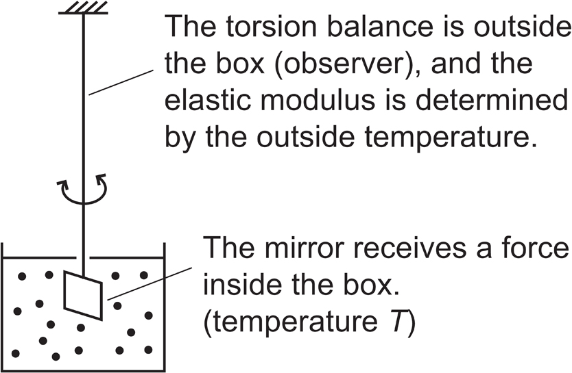
Extension of Kappler’s experiment: Measuring the local temperature. The mirror is inside the box, while the torsion balance is outside the box. The torsional force is determined by the temperature (T) of the gas inside the box; however, the torsional angle is determined by the elastic modulus of the torsion balance (outside temperature).
I would like to discuss our experimental results of the thermal bending motion of F-actin. Fig. 7.2 presents microscopic images, depicting the bending motion of F-actin with myosin head during ATP decomposition [7.1]. The top two rows represent the bending motion of F-actin without ATP decomposition, whereas the bottom two rows include ATP decomposition. Then, we could evaluate the bending modulus. When there was no ATP, we observed a normal bending motion of F-actin, from which we obtained its bending modulus. As there is no ATP, it is in thermal motion in equilibrium. Because the ATP decomposition starts when ATP is added, it is not in thermal equilibrium, but rather in a steady state, and energy is rapidly released. Where this energy is released is unknown. The bending motion at that time can be observed from the bottom two rows of Fig. 7.2 The time scale is given in the lower-right corner of the figure. If you note the difference in time between the top and bottom rows, you will find that the bending amplitude also increased with ATP decomposition, and the apparent cycle of the bending motion or the relaxation time are reduced.
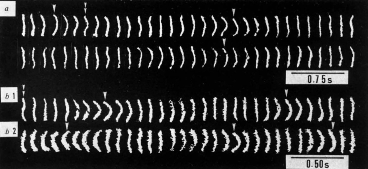
Dark-field microscopy images of F-actin in thermally bending motion7.1. The myosin molecules coexist to act on F-actin. A: The thermal equilibrium state of the bending motion of F-actin was observed without the ATP decomposition. B1 and b2: With the ATP decomposition (more energy was generated), the bending amplitude of F-actin was larger (i.e. more flexible) and its period was shorter (i.e. harder) than the corresponding values observed without the ATP decomposition. Therefore, the motion cannot be simply explained using the concepts of motions of flexible (large amplitude and long period) or hard (small amplitude and short period) materials. This figure has been reproduced from [7.1] with the permission of Springer Nature.
Examining Eq. 6.12, it is necessary to reconsider the temperature of the bending
motion. Has the average energy of the degree of freedom of the bending motion changed? You
might consider that it is different from the energy at room temperature
(
One explanation of this intuitively incomprehensible phenomenon could be that the relaxation time τ in Eq. 6.13 decreased; that is, the elastic modulus ε became larger. As there was no contact with any object, the viscosity ζ would be the same. Thus, we substitute Eq. 6.13 into Eq. 6.12 to arrive at Eq. 7.1.
| (Eq. 7.1) |
If the denominator ε in Eq. 6. 13 is large (τ becomes small), even though the bending amplitude is large, nothing else can be changed apart from increasing T. The experimental results could be explained by setting T to 4T, which is approximately 4 times higher than the room temperature7.2.
Although it is just one interpretation, it may be true. The bending elastic
energy is not limited to only the bending degree of freedom (
As the concept of temperature is defined in a macro level, if I postulate that the local difference in energy can be interpreted as owing to a high temperature, this may not be very convincing. However, we can use this concept of temperature, namely, “this degree of freedom has a high average energy.” F-actin was not fixed in a high energy state; it was moving appropriately, i.e. it became straight and then was bent repeatedly. When it became straight, the elastic bending energy was decreased, and that energy must have been transferred to somewhere. Hence, it cannot be said that the energy became large in that degree of freedom of F-actin. A high temperature does not simply imply high energy. A high temperature indicates a high energy and several degrees of freedom to interact (Table 7.2). When there is only one degree of freedom and no interaction, I do not refer to this as a high temperature. A surrounding environment must be present, that is, a degree of freedom to interact is necessary.
Concept of local temperature
| A high temperature implies high-energy with several degrees of freedom, with which the energy can be exchanged. |
Let us recall the dice and chip game with four chips and four boxes, first discussed in Section 2-4. The situation would be ideal for four degrees of freedom. F-actin received this bending degree of freedom during the bending. When F-actin became straight, there must have been a degree of freedom in the neighbors. Then, my claim is that if there are three or four degrees of freedom to receive the energy, we can use the current concept of temperature. Although a high temperature is correlated to high energy, it is not equal to the high energy. Temperature refers to energy that can be exchanged between several degrees of freedom, and the total amount of such energy is large. This is the meaning of high temperature. At this point, for example, we can ponder about the temperature of a fluctuation of a system. I think this is interesting, and I hope the readers also find it interesting.
Another example of local temperature is Feynman’s ratchet7.3. Fig. 7.3 is a diagram from “Feynman’s Lectures on Physics” [7.2], which I have reproduced here7.4. The figure in Feynman’s textbooks is not very clear. I think this figure facilitates a better understanding. In the Feynman’s figure, as the arrangement of the wheel (ratchet), vanes, and pawl is different, it is difficult to see the relationship between the movements. The figure here shows it better. It is not a big difference, but a matter of feeling. In Fig. 7.3, the upper left wheel is the ratchet, the pawl is attached to the ratchet wheel from the left, and the vanes are in the box at the lower right and connected to the ratchet by an axle. Owing to the Brownian or thermal motion, the ratchet can only rotate in one direction because of the pawl. The vanes are inside the box filled with a gas at temperature T1. The gas bombards the vanes, causing a clockwise or anticlockwise thermal motion of the ratchet wheel. Here, T2 is the temperature of the pawl, and K is the weight.

Feynman’s ratchet. A: Ratchet with asymmetric teeth. B: Vanes; as the vanes are in a box filled with gas at temperature T1, it is constantly bombarded by the gas molecules and receives random forces in clockwise and counterclockwise directions. C: Wall. D: Pawl with a spring inside. When the ratchet (A) rotates clockwise, the pawl retracts to the left, allowing the ratchet wheel to rotate. When the ratchet (A) rotates counterclockwise, the pawl interrupts the rotation. The temperature of the pawl is T2. K: Weight, the source of the force that attempts to rotate the ratchet counterclockwise.
Based on Feynman’s discussion of this microscopic ratchet, as long as there is no temperature difference between the system that rotates the ratchet wheel (Fig. 7.3; A, B) and the pawl (Fig. 7.3; D), this system does not rotate in one direction. As it rotates only if there is a temperature difference and there is heat flow associated with the temperature difference, it is not against thermodynamics. Moreover, when this rotation is converted into work, Carnot’s law also holds good, and hence, it provides an elegant interpretation. I recommend that you read Feynman’s textbook.
First, let us ignore the weight (Fig. 7.3; K). When the ratchet wheel rotates clockwise, the curve of its tooth gently pushes the pawl to the left so that it retracts to the left. As the pawl retracts only when pushed, after one tooth of the ratchet rotates clockwise with a clank, the pawl returns to its initial position, as shown in Fig. 7.3 On the other hand, in case of a counterclockwise rotation, as the structure of the wheel tooth prevents the pawl from being pressed, no matter how much the ratchet wheel attempts to rotate, it does not rotate in the counterclockwise direction. Therefore, the ratchet rotates clockwise only. However, if the temperature of the system that rotates the ratchet wheel (T1) and the temperature of the pawl (T2) are equal, the pawl could also retract accidentally owing to the thermal motion. When the pawl retracts owing to its own thermal motion, the Ratchet will rotate counterclockwise if there is a small weight on it (Fig. 7.3; K). Thus, the counterclockwise rotation is allowed according to a balance between the rotational thermal fluctuation of the ratchet and the reciprocating thermal motion of the pawl going in and out. In an extreme case, if the pawl does not undergo thermal motion and does not retract unless it is pushed, the ratchet rotates definitely in one direction.
For clarity, we consider the case the ratchet wheel is flat (Fig. 7.4). The thermal motion of the ratchet to the left and right pushes the pawl upwards. The pawl requires the energy ε when it is retracted by shrinking the spring because the energy of the spring has increased7.6. When the degree of freedom of the lateral movement of the ratchet receives energy ε, it pushes and retracts the pawl, and the ratchet moves to the right. The probability that the ratchet receives energy ε is exp(–ε/kBT1). T1 is the temperature that causes the thermal motion of the ratchet. In other words, T1 is the temperature of the heat bath behind the ratchet wheel. The pawl also has a heat bath with temperature T2. Then, the probability that the pawl will retract is given by exp(–ε/kBT2). In the absence of any weight, it will proceed with the difference between the two as the driving force.

Flattened version of Feynman ratchet. A flattened ratchet moves left and right owing to the thermal motion (temperature T1). The pawl moves up and down owing to the thermal motion (temperature T2)7.5
| (Eq. 7.2) |
In this case, Feynman deceives us by stating that v0 is the speed of motion when there is no such barrier, and these are simply written as the same coefficient v0. The meaning of this term is very difficult to understand. Therefore, it is assumed that these proportionality constants are the same. This is assumed, or rather, it must be assumed.
When a weight is applied, the energy to lift the pawl is ε and the energy to lift the weight K by l is Kl. Therefore, the total energy that must be received from the thermal motion with T1 is ε+Kl. Thus, the maximum height to which the weight can be lifted, and the maximum speed without the weight are expressed as functions of T1 and T2.
| (Eq. 7.3) |
Eq. 7.3 indicates that the Ratchet moves to the right of Fig. 7.4 (clockwise in Fig. 7.3) when T1 is higher than T2, and it moves to the left of Fig. 7.4 (counterclockwise in Fig. 7.3) to some extent, when T1 is lower than T2. It is very interesting; is it not?
Because I considered that the sliding motion of F-actin on myosin in muscles might be of ratchet type, I was interested in Feynman’s idea for a long time (approximately since 30 years ago), and I wanted to use the concept someday. Therefore, I proposed the ratchet mechanism in the original form, proposed by Feynman as the mechanism of the sliding movement of muscles.
After Feynman, various ratchet mechanisms were proposed by several researchers. As it is not ideal to consider the temperature difference, not everyone was convinced, and several more elegant ideas were introduced. Many of these concepts were published in “Physical Review Letters” [7.3,7.4], and there was widespread interest among the researchers. Reviews and reports on this subject were also published in “Nature,” journal and it became a popular topic. As the first prototype was by Feynman, it is still the best. It is only Feynman’s original model that can describe exactly the amount of energy applied and amount of heat generated. Although there are several other elegant and seemingly elegant models, the energy calculation cannot be logically performed. Although this statement could be an exaggeration, these models need to be further contrived to allow for a logical calculation. In Feynman’s model, when the ratchet moves one step in the clockwise direction, the pawl receives an energy ε and is lifted. As the spring attached to the pawl shrinks tightly, it returns to its initial position. Thus, eventually all of ε is converted into heat. Therefore, to move one step, ε does work out to be equal to Kl and heat is transferred from a higher temperature T1 to T2. Therefore, the amount of heat per step is constant.
Let us assume a high local temperature T1; in other words, the temperature of the ratchet is high. If we state that the temperature of actin is high, no one will be convinced. In our earlier discussion on temperature (in Section 7-2), when we indicated that the temperature was four times the body temperature (although I was very much pleased with that), everyone disagreed saying “it seems that it is not hot by touch at all!” or “no way! it cannot be that the actin temperature is high!” One reason why not everyone agreed was that it is generally that temperature is a macroscopic attribute, and hence, it is difficult to think that there is a special temperature at a specific degree of freedom. Another reason is that, it is believed that proteins cannot store such high energy anywhere, which means that the energy must be “consumed” (that is, dissipated around). These are the reasons why most were not convinced. This is a very difficult topic. Therefore, next, I will demonstrate that this temperature is measurable.
I would like to discuss the fluctuations of the sliding motion of F-actin. Although this topic was investigated in a published report [7.5], it did not generate much interest. Let us assume that we have the following motion. My apologies to those who are unfamiliar with actin and myosin; however, the following is based on an experiment we have been conducting since the 1990s [7.1,7.6].
As shown in Fig. 7.5, an F-actin molecule was glued to the tip of a thin glass needle (left side of Fig. 7.5). As this was done in water, the surrounding medium was water. The left end of F-actin was fixed (on the thin glass needle), and F-actin was in water. In contrast, myosin molecules were fixed onto a glass plate, on which F-actin was gently placed. When ATP was added, myosin broke down the ATP to produce energy, and when F-actin performed a sliding motion, it was pulled to the right. When it started to move quickly, the needle bent as shown in the figure, and stopped when it balanced the generated force. F-actin was visible under the microscope. This achievement was attributable to Sho Asakura7.7 and Nagashima Hajime [7.7]. If the number of myosin was low, the force would fluctuate. If the force fluctuated, the needle would fluctuate. This fluctuation could be observed using a microscope. Given that this displacement was measured in nm, the force exerted on the needle was measured in piconewtons. We observed the displacement of the tip of the needle in nm. If we attach a small grain to the tip of the needle and carefully observe its position, we can measure the force fluctuation in piconewtons. In terms of muscle biology, even though it did not slip and stopped already, shaking occurred because its power fluctuated.

Measurement of the fluctuation of F-actin sliding motion. Myosin was fixed on a slide glass and F-actin attached to the tip of a thin glass needle (left side in the figure) was placed on it. If F-actin was at temperature T1, the glass needle fluctuated as if it was at temperature T1.
Therefore, when adopting this model7.8, if the lower linear ratchet in Fig. 7.4 was F-actin, it would go to the right. The needle attempted to pull F-actin to the left. As a result, it was balanced at the point, where the system was at the moment and stopped. Movements to the left and right became equal and stopped. However, since it was a stochastic process, it occasionally moved back and forth maintaining a constant average position. The back-and-forth motion would depend on the observation. This back-and-forth motion was that of the leftmost needle in Fig. 7.5 However, the needle had its own temperature as it was located far outside the position of myosin. As the needle had a filament, F-actin, a force was generated between F-actin and myosin. Using this model, we calculated the amount of fluctuation of the needle. Then, if it was at the high temperature T1, the needle also fluctuated. Applying this model, as the needle at the left end of the figure was outside, there was a ratchet mechanism at the location of F-actin and myosin, and T1 acted on F-actin. Although the needle was located far outside, its fluctuation was akin to that of the local temperature of F-actin, that is, the temperature of the ratchet mechanism.
The needle is bent at the center of oscillation, and it swayed around with the center as the bent state (not around the straight line, but around the bend). If the fluctuation width is δ and elastic constant of the glass needle is κ, the following equation is applicable.
| (Eq. 7.4) |
In this case, T1 is the temperature of the ratchet mechanism, which is in a virtual high temperature state. In other words, the temperature of the high temperature side can be theoretically determined.
Therefore, if we measure the fluctuation of the tip of the glass needle, we can measure the virtual temperature of F-actin. In Feynman’s case, it was a micro ratchet. However, as the temperature in this instance was that of the gas, it was a macroscopic temperature. Therefore, although the Feynman ratchet temperature in Fig. 7.3 was a macroscopic temperature, the temperature of the ratchet mechanism in Fig. 7.4 was not the macroscopic temperature, but rather, the temperature of the lateral motion of the mechanism. It was the local temperature. The whole system itself, consisting of this F-actin and the needle, was at room temperature. The local temperature appeared to be crucial in this case. Therefore, the most important point is that if we measure the fluctuation of the tip of the glass needle in Fig. 7.5, we can effectively measure T1. Hence, in my paper, I wrote “T1 is measurable”. This is an important point. If there are local temperature and energy seeds like these, it would be appropriate to measure it in this way. For now, if the bending motion of F-actin in Fig. 7.2 is interpreted in terms of the temperature, this means that the latter could be measured by observing the bending motion. However, it would be ideal if there was another approach to allow for its confirmation. Thus, even such a local temperature is not a completely fictional parameter that cannot be measured.
However, even if I go to the researcher’s laboratory described in Ref. [7.1] and attempt to measure the temperature, it would be impossible. The reason why it cannot be measured is that because the actin-myosin bond dissociation fluctuates, the bond is easily broken and myosin jumps elsewhere. The bond shows association and dissociation fluctuation, i.e., actin pops from one myosin to another myosin. As this fluctuation takes place in the experiment, it does not move. Hence, the experimental measurement is virtually impossible. Although the fluctuations operate far more effectively in the dissociation of the actin-myosin bond, kinesin and microtubules may not necessarily be captured in it. Hence, I am still hopeful about them.
To distinguish between simple tension fluctuation and thermal fluctuation (energy fluctuation), we must prove that the right side is a constant, even if a needle with a different elastic constant is used, and the elastic constant (κ) and δ of Equation 7.4 are changed. However, we cannot simply measure this and say that we have forcibly measured T1. In the case of tension fluctuations, the mean of κ times δ, i.e., (κ⟨δ⟩) is significant; however, in the case of energy fluctuations, the mean of κ times δ squared, i.e., (κ⟨δ2⟩) is significant. This must be proved. The experiment has to be done under the condition of changing the needle to change the modulus of elasticity or, if using optical tweezers/laser, changing the intensity of the laser7.9.
Thus, from these two examples, my claim is that it is possible to determine the temperature of the system that causes the fluctuation. This temperature has various uses, not as a macroscopic temperature, but as the local temperature, particularly in systems that convert energy. However, even though it is simply used for confirmation without any specific use in an equilibrium system, my assertion is that this method can be used in energy generation systems. If one can think of this in another case instead of actomyosin sliding motion, it may have surprising uses. In summary, if we can prove that energy fluctuations are fixed, and fluctuations with a constant energy width that are not tension or displacement fluctuations are present here, we can determine the temperature. This means that the temperature can be defined.
It should be noted that, in Figs. 7.5 and 7.4, although the temperature corresponding to T1 can be measured, that corresponding to T2 cannot be measured. You may wonder why only T1 can be measured. I also wondered the same thing and proceeded to theoretically examine this conundrum. I am not sure why this is the case, and would appreciate it if someone would theoretically study this problem. It is still unresolved. What is known is that T1 is higher in energy, because it is at a higher temperature. Therefore, it is the F-actin (T1) that has the energy. A glass needle is attached to T1 (F-actin), as shown in the left side of Fig. 7.5 Considering that because F-actin of Fig. 7.5 corresponds to the ratchet in Fig. 7.4, T1 can be measured.
This is related to our earlier topic on ATP hydrolytic enzyme (Section 6-4). Myosin is attached to an energy source called ATP, ATP+H2O decomposes into ADP and P on the myosin molecule, and they remain attached. If actin does not come into picture, they remain attached and will not separate easily. Nevertheless, they finally separate after a few seconds. Thus, as the time duration that I mentioned earlier, that is, the time during which ATP remains attached is of the order of a few seconds, it can be measured slowly. I previously indicated that those few seconds have an exponential function distribution. It is a long macro time. After a few seconds, ADP will stochastically become separated, and the ATP decomposition reaction will end.
When actin is present, a process that took a few seconds, now leads to an interaction with actin in a very short time interval, and separation is initiated. The separation only takes an order of 1~10 ms and the reaction proceeds. Thus, actin arrives at a position, where ADP and P are attached to myosin and start interacting with them. Hence, at the time, I was hoping that there might be some energy transfer from myosin to F-actin. However, this model was not common. Moreover, unfortunately, there was no clear evidence t no evidence to support this move at this time.
Sugie Fujime7.10 from Nagoya experimented with actomyosin for a long time. In particular, he conducted research on the very fast sliding motion of (stonewort) Nitella’s7.11 actomyosin. There is a very interesting paper by Fujime [7.8]. It reported that although ATP became ADP and P on myosin, it did not easily progress after that, and the longer it was in equilibrium, the faster F-actin slid on myosin. Normally, it is expected that the faster ATP hydrolyses, the faster it slides. The higher the actomyosin and ATP hydrolyzing ability, the faster the slide. However, there was no correlation, and it was inconclusive. What correlated with it was the lifetime of ATP. When the aforementioned lifetime wherein the hydrolysis did not occur easily was longer, it worked better, and yielded surprising results, such as working fast and causing them to move quickly.
I thought that, perhaps, the energy accumulated by myosin was accumulated in a stable manner, and that when actin was introduced, it transferred the energy in an ideal manner, and slid quickly so as to transfer it without wastage. Although I think this constitutes good data, it is proportional to 1/(speed), the direction of the slowly decomposing ATP, which is completely counterintuitive. That is, it becomes faster in proportion to the life-time τ. It becomes a straight line when two experiments are combined—one that used various ATP analogues [7.8] and another, a genetic engineering experiment, conducted by James A. Spudich7.12 [7.9], wherein myosin was modified. Thus, the more stable the ATP hydrolysis energy was on myosin, the faster the actin slid. Hence, probably, the energy accumulated in some degree of freedom, or rather, in a few degrees of freedom. However, not many people may agree that this is actin. The actin bending experiment [7.1] mentioned in Section 7-2 was indeed an experimental evidence that the degree of freedom of actin bending was shifted. In this case, myosin was not stopped; instead it floated freely. In the case of non-fixed, free-floating myosin, the energy was transferred to the bending movement of F-actin. In that case, each F-actin molecule decomposed ATP once per second, which meant that ATP was decomposed at that rate, at which, if it was dissipated in 1 ms or faster, that level of activation would not have been possible. Hence, it is obvious that energy was transferred elsewhere.
The discussion in this session is related to the previous topic, and at the same time, leads to Brownian motion in the next chapter. Table 7.3 shows a famous relational expression (fluctuation dissipation theorem). In short, there is a proportionality relationship between the response to an external force and magnitude of spontaneous fluctuations. The response to an external force, that is, the response to environmental changes, such as the amount of bending (Eq. 7.4) or the amount of twisting (Eq. 6.10) when a force is applied, is proportional to the mean-square of the fluctuations owing to spontaneous thermal energy when an external force is not applied. This is a well-known formula of statistical mechanics.
Fluctuation dissipation theorem
| There is a proportionality relationship between the response to an external force (sensitivity) and magnitude of spontaneous fluctuations in a certain environment. | ||
|
|
||
| Spontaneous fluctuation in a certain environment: | Large | Small |
| | | | | |
| Sensitivity to environmental change: | Large | Small |
In Eq. 6.10, the response to an external force component is 1/K (the elastic modulus of torsion), which is proportional to the mean-square of the spontaneous torsion (<θ2>) when an external force is not applied. As the fluctuation is large when the temperature is high, it is proportional to the square of the spontaneous fluctuation. The mean-square of the spontaneous fluctuation of the angle of torsion is proportional to the ease of twisting when an external force is applied. It is also proportional to the temperature. Conversely, a system with no spontaneous fluctuations does not respond, even when an external force is applied.
I explain this theorem with electrical conduction experiments. This theorem should be applied to an equilibrium state. Here, electrical conduction in a steady state is discussed. In terms of electrical conduction, the current that flows when an external force (potential difference) is applied is proportional to the current that fluctuates internally when a potential difference is not applied. In other words, it is proportional to the current fluctuation. The spontaneous fluctuation of current was measured by Johnson7.13 in 1928. This experiment is now popular in academic course experiments in universities. It is a useful experiment, wherein the relationship between the spontaneous fluctuation of current and electrical resistance in a steady state can be demonstrated using an ordinary wire filament. In the case of thermally bending motion of F-actin, a rod of F-actin is in equilibrium state when bent. The rod that can be easily bent exhibits a large fluctuation in amplitude when it is spontaneously shaken. These phenomena are observed to be similar.
I feel that the fluctuation dissipation theorem would be extendable to an educational creed. If one’s belief is rigid, it is impossible for the person to respond sensitively to changes in the environment. People who are sensitive to environmental changes are better off having no belief than having beliefs.
I think this analogy is instructive. People who can spontaneously respond to a certain environment would be sensitive to environmental changes by themselves. That is, the spontaneous fluctuations in a certain environment and sensitivity to environmental changes would be positively correlated even in humans. If the relation is inverse, it would be inconsistent with the natural world. Thus, the more the fluctuations, the more easily one responds to external stimuli. I do not emphasize that a person who responds more appropriately to a change is better. Nevertheless, this analogy is quite interesting.
Long ago, when a research facility for molecular biology7.15 was established in Nagoya University, there was no molecular biology department in that university yet, and graduate students came from various departments. Certainly, there were students from the biology department; however, students from other departments, such as physics, chemistry, engineering, agriculture, medicine, and mathematics were present. At that time, I trained students for the first half year until the summer vacation. The students from the physics department did not know how to use pipettes. A student, now a famous professor, was using it upside down7.16. Another student, also a famous professor now, was attempting to dissect a crab’s muscles; however, it turned out to be its nerves7.17. Thus, we were attempting to learn things from each other. In graduate schools, learning from each other is most effective. Listening to a teacher’s lectures is often not very effective. Therefore, in graduate school, it is good for students, who come from various departments, to teach and learn from each other. As they acquire specialized knowledge in the undergraduate studies, it is worth teaching people who come from different fields. I still feel nostalgic about those days. Therefore, I think it would be great if people from different fields come together.
In the final lesson of the course, there was marine life training at the marine laboratory in Toba7.18 and started with the observation of cell division of sea urchins. When we said, “Let us start marine training as the final lesson!”, the students happily attended it. However, from some point, some students started saying “we have seen the cell division of sea urchins on television; so we do not want to go for marine training!”, and I was taken aback. I did not know what the readers think. I understand that they wanted to perform the front-line experiments sooner, and that is fine. However, I think that learning from a video is different from working hands-on. Although television has developed significantly and provides useful content, it is completely different from your own experience. It is meaningless if you do not do it yourself.
Therefore, even in the case of the dice and chips experiment, please do not think that it is fine as you have heard about it; but please try it yourself. I think that, once you start, it will become too interesting to stop.
7.1 Translator’s note: The figure legend is abbreviated because it repeats the explanations in the text from the original Japanese textbook.
7.2 Original note: As T is the absolute temperature, the room temperature is approximately 300 K, and four times this value is 1200 K, which means 4T is approximately 900°C.
7.3 Translator’s note: It is commonly known as Brownian ratchet.
7.4 Translator’s note: Fig. 7.3 was re-redrawn by us based on Oosawa’s hand-drawn diagram.
7.5 Translator’s note: the figure legend has been abbreviated because it repeats the explanations in the text from the original Japanese textbook.
7.6 Original note: See references [7.5] and [7.10] for more details.
7.7 Original note: Sho Asakura is a Professor Emeritus at Nagoya University. He conducted a number of advanced studies, including “Asakura and Osawa’s force,” described later.
7.8 Original note: Vale and Osawa model; see Section 9.5 of [7.11].
7.9 Original note: Instead of a glass needle, attach beads and fix them at one point in water using devices called laser tweezers. By changing the intensity of the laser output, the strength of the fixing can be adjusted.
7.10 Original note: Sugie Fujime is a former assistant professor, Faculty of Science, Nagoya University.
7.11 Original note: Japanese name—Furasumo, a floating aquatic plant (algae).
7.12 Original note: James A. Spudich. Professor at Stanford University. Specialist in single molecule measurement
7.13 Original note: John Bertrand Johnson (1887–1970), Former researcher at Bell Labs.
7.14 Translator’s note: In the original Japanese book, this is not a part of a coffee break but of the main text.
7.15 Original note: This refers to the molecular biology research facility of the Faculty of Science, Nagoya University, established in 1961. A graduate school was established in 1963. It was later integrated with the Department of Biology and became the Department of Life Sciences.
7.16 Original note: A measuring pipette is a glass tube with a scale for measuring liquids, which is sucked by mouth. The scale becomes bigger as it goes from 1 through 2 to 3 from the top to bottom. It is noteworthy that it is easy to get confused between the top and bottom of the pipette.
7.17 Original note: As muscles and nerves of living crabs are white and transparent, unless you are used to viewing them, they are difficult to differentiate. Incidentally, the sarcomeres (periodic structures composed of actin and myosin fibers) of crab muscles are tens of μm long and facilitate optics related research.
7.18 Original note: A marine biological laboratory of Nagoya University at Sugashima island in Toba, Mie Prefecture.