Abstract
Recent small-angle X-ray scattering (SAXS) for biological macromolecules (BioSAXS) is generally combined with size-exclusion chromatography (SEC-SAXS) at synchrotron facilities worldwide. For SEC-SAXS analysis, the final scattering profile for the target molecule is calculated from a large volume of continuously collected data. It would be ideal to automate this process; however, several complex problems exist regarding data measurement and analysis that have prevented automation. Here, we developed the analytical software MOLASS (Matrix Optimization with Low-rank factorization for Automated analysis of SEC-SAXS) to automatically calculate the final scattering profiles for solution structure analysis of target molecules. In this paper, the strategies for automatic analysis of SEC-SAXS data are described, including correction of baseline-drift using a low percentile method, optimization of peak decompositions composed of multiple scattering components using modified Gaussian fitting against the chromatogram, and rank determination for extrapolation to infinite dilution. In order to easily calculate each scattering component, the Moore-Penrose pseudo-inverse matrix is adopted as a basic calculation. Furthermore, this analysis method, in combination with UV–visible spectroscopy, led to better results in terms of accuracy in peak decomposition. Therefore, MOLASS will be able to smoothly suggest to users an accurate scattering profile for the subsequent structural analysis.
Significance
Small-angle X-ray scattering (SAXS) combined with size exclusion chromatography, SEC-SAXS is an effective method to analyze the solution structure of the target molecule mixed in a polydisperse solution. SEC-SAXS continuously measures more than hundreds of data in a single measurement while the sample solution flows. In this study, we developed the analytical software MOLASS to automatically analyze such a large amount of SEC-SAXS data by combining UV-visible spectroscopic data measured simultaneously with SAXS. MOLASS solves several issues that arise during the measurement and achieves automated analysis using linear algebra techniques.
Introduction
Recent small-angle X-ray scattering for biological macromolecules (BioSAXS) techniques have enabled the elucidation of unique structures of molecular complexes in solution. To reliably solve high-order solution structures using SAXS measurements, it is important to analyze the target molecule with monodisperse conditions complying with SAXS publication guidelines [1]. In order to achieve this condition, a SAXS measurement system combined with size-exclusion chromatography (SEC-SAXS) has been developed [2], and its use has become widespread in the last decade. The proteins in solution flow through a gel-filtration column and are continuously injected into a SAXS sample cell or capillary. Continuous flow mitigates the effects of radiation damage, and size-exclusion chromatography allows for the exploration of each monodisperse component. A high-speed readable 2D image detector contributes to the realization of these measurements, and various facilities worldwide have established these SEC-SAXS measurement systems [3–6]. Because measurement of the molecular complex under monodisperse conditions, which had been difficult before, is achieved relatively easily using SEC-SAXS, the number of BioSAXS analysis setups at synchrotron radiation facilities is increasing with a scientific interest in this method [7]. Disadvantages of SEC-SAXS include the need to analyze more than hundreds of scattering intensity images at once unlike conventional methods and the ability to choose the proper frame regions that correspond to the baseline and the target molecule scatterings. Aside from the selection of the baseline region, it might be difficult to automate the determination of the frame region suitable for processing from the large number of scattering intensity profiles that constitute the elution peak of the chromatogram. When done manually, the selection of these parameters might be subject to user bias.
In order to carry out such complicated analysis efficiently, several data analysis software programs have been developed and used. CHROMIXS is one of the most basic modules included in the ATSAS software package [8–10]. This software automatically selects the regions in the images that correspond to the buffer and sample scattering profiles. The selected data frames for the buffer and sample are averaged individually, and the buffer intensity is automatically subtracted from the sample intensity. DATASW is another user-friendly software that performs basic analysis, including calculating forward scattering (I(0)), the radius of gyration (Rg), the maximal dimension (Dmax), and the estimated molecular weight for each frame [11]. These parameters are plotted against the number of frames to allow users to select suitable regions for averaging based on those results.
However, some data sets obtained at synchrotron facilities are further complicated by effects from radiation damage to the sample or impurities in buffer components. Because sample cell window fouling generated by these effects increases the scattering intensities at the small-angle region during measurement, users have to carefully avoid these problems. DELA corrects the scattering intensities in the small-angle region to reconstruct the certain scattering profile with a high enough signal-to-noise ratio using singular value decomposition (SVD) and the linear combination of Guinier optimization [12]. The analysis is processed based on the Guinier approximation, which can also reduce the scattering profile derived from artifacts. Another approach used to avoid artifacts introduced by fouling is to correct the baseline for each scattering profile based on the baseline variation within each chromatogram. The HPLC module of US-SOMO modifies the baseline by assuming that the scattering intensities of the baseline gradually increase with the fouling of the capillary used as the sample cell [13,14]. The module based on this integral baseline correction concept omits the extra baseline scattering component, which is proportional to the sample intensity from the whole scattering data set.
Another problem SEC-SAXS users face is the deconvolution of a chromatogram with multiple overlapping peaks. Because peaks that cannot be completely separated by size-exclusion chromatography are composed of multiple scattering components, a method for separating each scattering component is required. One of the methods to separate components corresponding to individual peaks from a chromatogram with multiple overlapping peaks is the fitting of multiple modified Gaussians, which was proposed for use in analyzing size-exclusion chromatography data [15,16]. US-SOMO adopts a method to decompose multiple components of overlapping peaks by fitting them with the modified Gaussian functions. By contrast, EFAMIX and the LC module in the BioXTAS RAW use model-free decomposition with evolving factor analysis (EFA) [17–21]. This method searches for the start and end points of each component on the chromatograms using the changes in the singular values. Scattering profiles for each component are obtained using an iterative approach that uses the basis vector of the singular value. These software programs have been developed and updated at each synchrotron facility to address specific analysis needs, and users can select and utilize one suitable for their individual processing needs. The use of these programs is very advantageous for streamlining the analysis of SEC-SAXS data.
With reference to the various software developed to date and described above, we propose four essential problems that need to be resolved in the development of automated-analysis software for SEC-SAXS data: 1) correction of baseline drift; 2) consideration of concentration-dependent effects generated by interparticle interference; 3) separation of complicated peaks; and 4) easy-to-use software with automated analysis that eliminates user bias. We discuss each of these problems in turn. 1) It is presumed that two main causes produce baseline drift. The first is from the stability of the instrumentation, such as X-ray beam intensity and the pump system, and the second is from radiation damage to the sample. Regarding the former, because SEC-SAXS measurements take longer than conventional SAXS, they are susceptible to long-period fluctuations in beam intensity and pump pressure. For the latter, the addition of radical scavengers, such as reductants, to the sample solution mitigates this effect, thereby reducing the fouling of the capillary or sample cell quartz glass windows [7,22]. However, it is often desirable in complex molecular systems to avoid an artificial influence on the target molecule that is generated by the addition of the scavengers. The effects from radiation damage should be suppressed by reasonable measurement and sample conditions; however, if the damage cannot be avoided experimentally, it would be necessary to solve this problem with an analytical approach. Therefore, baseline correction is essential to obtain the proper scattering profiles for the target molecule. 2) The currently available software programs do not take into account the effects of concentration dependence. The concentration of the sample may be diluted to 1/3–1/10 of the initial concentration depending on the volume of the SEC column, the starting concentration of the sample, and the volume of the sample injected. However, it is well-known that the concentration-dependent effect strongly depends on the solute conditions [23]. Therefore, it is difficult to conclude that the target molecule is in a state equivalent to infinite dilution in the SEC elution peak in all SEC-SAXS experiments. In order to obtain the appropriate scattering profile of the target molecule, protein concentration information must be used to remove concentration-dependent components from the original scattering profile, as is done for conventional SAXS analysis. Hence, SEC-SAXS measurements must be carried out in conjunction with UV–visible spectroscopy to accurately evaluate the sample concentration, and this spectroscopic device must be installed as close to the SAXS measurement position as possible. 3) In recent years, most SAXS users seek to analyze higher-order complexes, including interactions between proteins and chemical compounds or other proteins. In such cases, each minor component contained in the sample solution will be observed as distinct peaks in the SEC analysis, and unfortunately, these peaks often overlap with the peak derived from the analytical target. This problem can sometimes be solved by selecting a gel-filtration column with sufficient separation ability and by optimizing solution conditions and sample preparation conditions. However, in many cases, though these strategies mitigate the situation, it is very difficult to completely solve the problem. In order to succeed in analyzing the scattering profile derived only from the structural state of the target, the ability to accurately decompose the mixed scattering components is indispensable. 4) The advanced analyses described above in bullets 1), 2), and 3) allow users to determine and input initial parameters manually, but this task can be daunting, in particular for novice users, because users may not know which initial parameters are best for their sample. Moreover, in general, the appropriate initial parameters must be selected without bias in order to conduct an accurate analysis. Hence, software for SEC-SAXS analysis needs a function that can automatically select non-biased parameters. The strategy of automation combined with a user-friendly interface is the most effective way to not only perform high-throughput analysis but also properly correct the parameters without user bias. This approach would support a wide range of various-leveled BioSAXS users, from beginners to experts.
In order to address the issues above, we developed the software MOLASS (Matrix Optimization with Low-rank factorization for Automated analysis of SEC-SAXS) to analyze SEC-SAXS data. MOLASS outputs the scattering profiles in the infinite dilution state for all the identified scattering components using whole background–subtracted data from SEC-SAXS combined with UV–visible absorption spectra data. A preliminary version of this software, containing simple baseline correction functions, mapping between SAXS intensities and UV–visible absorbance, and extrapolation to infinite dilution, was already released [24]. Here, we updated the program modules to obtain further solution optimization by solving the general low-rank factorization problem using matrix-based data analysis for SAXS intensities and concentrations calculated from UV–visible absorbances. Additionally, all processes, including baseline correction, mapping optimization between SAXS intensities and UV–visible absorbances, peak decomposition fitting with the modified Gaussian function, and rank determination of each decomposed peak, were automated. In this paper, we describe these modules in detail and present the results from using MOLASS to analyze multiple standard SEC samples.
Materials and Methods
Experimental Procedure
Lyophilized ovalbumin from chicken egg white and cytochrome C from horse heart were purchased from Sigma-Aldrich (A7641) and Nacalai Tesque (10429-55), respectively, and were resuspended in a 10 mM HEPES, pH 7.0, and 50 mM NaCl buffer. Initial concentrations of these samples were adjusted to 5.7 mg mL–1 and 25 mg mL–1, respectively. The injection volume for these samples was 200 μL. A Nexera-i HPLC system (SHIMADZU) with a Superdex 200 Increase 10/300 GL column (GE Healthcare) (ovalbumin) or a Superdex 75 Increase 10/300 GL column (GE Healthcare) (cytochrome C) was used to isolate the monodisperse proteins. The columns were pre-equilibrated with sample buffer. The flow rate during the chromatography run was 0.2 ml min–1 (ovalbumin) or 0.3 ml min–1 (cytochrome C). The SAXS experiments were performed at BL-15A2 of the Photon Factory (PF) in Tsukuba, Japan. The exposure time was set to 4 sec for ovalbumin and 3 sec for cytochrome C for each frame. 800 and 1100 frames were collected for ovalbumin and cytochrome C, respectively. The wavelength and camera distance were set to λ=1 Å and about 2.5 m, respectively. The conventional SAXS measurement of Cytochrome C was also performed at BL-10C of the PF. The wavelength and camera distance were λ=1 Å and about 1 m, respectively. The exposure time for each frame was set to 10 sec, and 20 frames were recorded for each concentration. The concentration series of cytochrome C are 1, 2, and 4 mg mL–1.
Lyophilized aldolase and thyroglobulin were purchased from GE Healthcare (Gel Filtration HMW Calibration Kit). These samples were resuspended in a 10 mM HEPES, pH 7.0, and 120 mM NaCl buffer. Initial concentrations before injection on the column were approximately 5 mg mL–1. The injection volume for these samples was 200 μL. An ACQUITY UPLC H-Class system (Waters Corporation) with a WTC-030S5 column (Wyatt) for aldolase and a Nexera-i HPLC system (SHIMADZU) with a Superdex 200 Increase 10/300 GL column (GE Healthcare) for thyroglobulin were used to isolate these proteins. The column was pre-equilibrated with the sample buffer. The flow rate during the chromatography run was set to 0.05 mL min–1 for aldolase and 0.1 mL min–1 for thyroglobulin. The SAXS experiments were performed at BL-10C of the PF. The exposure time and the number of frames were set to 20 sec for each frame and 300 frames, respectively. The wavelength and camera distance were set to λ=1.5 Å and about 2.0 m, respectively.
Details of the SEC-SAXS/UV-visible spectroscopy system and the basic process of the measurement data are described in the supplementary information. The extinction coefficients for these proteins were also calculated using the protparam web tool [25].
Software Implementation and Operation
MOLASS is a Python-based program enhanced with external modules such as numpy, scipy, matplotlib and scikit-learn. This program is available on 64-bit Windows 10 and later operating systems. Users can download this software (.zip file), including tutorials and manuals, from http://pfwww.kek.jp/saxs/MOLASS.html. Because the file also contains the source codes written in Python, a software development expert can refer to and edit these source codes.
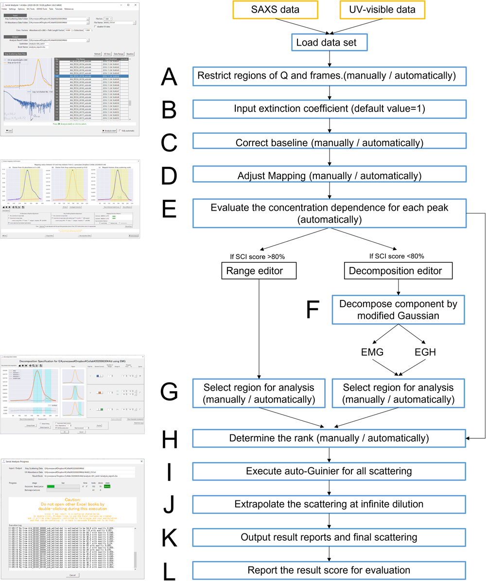
The operational flow of the main GUI and functions are shown in Figure 1. The resultant analytical processes, including the Guinier analysis and the derivation of the scattering profile extrapolated to the infinite dilution, are summarized in the “report.xlsx” file. In order to evaluate the accuracy of the automatic Guinier analysis of each scattering profile, several quality scores were established. Details for the Guinier analysis quality scores are described in a previous report [24]. This directory contains the extrapolated scattering profile and the scattering profile component that is dependent on the sample concentration. If the ATSAS program package [10] was installed, AUTORG, ALMERGE, and DATGNOM4 are also running [26,27]. In that case, the processing results from the ATSAS modules, including the scattering profiles extrapolated to the infinite dilution computed by ALMERGE, are output together with those of MOLASS. If users desire to calculate the electron density map using the program DENSS [28], it can be accessed in the start menu of the main GUI.
This software selects the final peak region to calculate the extrapolated scattering profile for the ascent and descent sides of the peak. This will determine whether the non-targeted components are contained on either side or not. It is also possible to manually combine both the ascent and descent sides into a single calculation.
Computational Algorism
Basically, the data sets from SAXS and UV–visible spectroscopy are treated as the matrix data (Frame No., Q-vector or wavelength, and intensities or absorbance). The concept of our software is to conduct the optimization of SAXS and UV–visible absorption data as low-rank matrix factorization problems, which is referenced to a method proposed to analyze chromatograms composed of multivariate UV-visible data in the field of chromatography [29]. MOLASS processes the matrix data according to the analytical flow chart in Figure 1.
Determining the Scattering Component from the Whole SEC-SAXS Data Set
Assuming that the whole data set M (n-th Q-points×m-th data frames) contains i components, matrices can be described as follows:
| M≡I1Q1⋯ImQ1⋮⋱⋮I1Qn⋯ImQn=P1Q1⋯PiQ1⋮⋱⋮P1Qn⋯PiQnC11⋯Cm1⋮⋱⋮C1i⋯Cmi≡P∙C | (1) |
Pi(Q) and Ci are the scattering profiles of i-th components and the concentration series for each frame number, respectively. In addition, Equation (1) can be extended as follows if the concentration dependence, including the interparticle interference effect, must be considered:
| M≡I1Q1⋯ImQ1⋮⋱⋮I1Qn⋯ImQn=A1Q1⋮A1Qn B1Q1⋯AiQ1⋮⋱⋮ B1Qn⋯AiQn BiQ1⋮BiQnC11C112⋯⋯Cm1Cm12⋮⋱⋮C1iC1i2⋯⋯CmiCmi2≡P∙C | (2) |
In these matrices, the i-th scattering component (Pi) can be described as PiQ=AiQ×Ci+BiQ×Ci2, assuming that the concentration dependence term Bi(Q), except for the form factor Ai(Q), is proportional to the second order of the concentration with reference to the SAXS basic theory [30]. If we can determine the concentration of each component, we can optimize the P components by calculating the following least square function:
This minimization of the optimized P matrix corresponds to solving the Moore-Penrose inverse matrix [31,32] as follows:
Hence, each scattering component P can be calculated if the concentration component is already known. When UV–visible absorption spectra for each scattering profile are simultaneously recorded at the same (or a very near) position, and the concentration information is described as matrix C containing all the components, all the scattering components can be resolved.
To calculate the error in the final scattering profile, we used linear propagation for the whole process, from the starting data (M) to the final scattering data (P). Basically, the linear propagation from matrix M to matrix P can be described as P=M·X. The error in P (E~) can be described as follows using the error of M (E) and the transformation matrix X: X=M+·P and E~ij=(E∘E)∙(X∘X)ij where the circle and dot denote the multiplied function for each element and matrix, respectively.
Mapping Optimization between the SAXS and UV–visible Data
The detail of baseline corrections shown in Figure 1C is described in the supplementary information. After correcting the baselines for the SAXS and UV–visible data, the horizontal axis (Frame No.) for both chromatograms has to be aligned. In order to align the horizontal axis, a mapping optimization process between the SAXS and UV–visible data is performed as follows: flame No.X-ray=a×(flame No.UV-visible)+b, where the parameters a and b are scaling factor and offset, respectively. This process allows for the UV–visible Frame No. to align with that of the SAXS data (Figure 1D). Although the software recognizes several peak maximums and half-intensity of peak maximum positions as initial alignment positions, second-derivative extremum positions are subsequently added for results with a single peak with an additional shoulder component. If the correlation coefficient for the mapping parameters (a, b) and the similarities between these peak forms are not improved by addition of these features, the mapping parameters between the intensities at Q=0.02 Å–1 (I0.02) and scaled absorbance at λ=280 nm (Abs280) can be further aligned by minimizing I0.02-Abs280×scale2, subject to a, b, and scale factors.
When the chromatograms that were processed after baseline corrections and mapping optimization are superimposed on the same figure, the matching score, a single component indicator (SCI) score, is considered. This score describes the ratio of the variance region, where the difference between the chromatograms for I0.02 and the SAXS data and that between scaled Abs280 and UV–visible data are within 2% of the maximum peak intensity in all regions, including the foot of the peak. The score under approximately 80 suggests that a different component may be contained in the peak region due to the differences between the extinction coefficients. For data with a SCI score >80, it is not necessary to decompose peaks using a Gaussian model; thus, the extrapolated scattering profile is calculated directly using both the X-ray scattering data and absorbance obtained from UV–visible. In this case, the range editor is available as shown in Figure 1E. The peak decomposition process using exponentially gaussian hybrid (EGH) and exponentially modified Gaussian (EMG) shown in Figure 1F are also explained in the supplementary information.
Rank Determination on the Region Selected for Analysis
To recognize whether concentration dependence was included or not, the matrix rank for each component has to be determined (Figure 1H). Taking a single peak as an example, it can be described as rank=1 if no concentration dependence exists. By contrast, the rank of this component may be 2, assuming that the scattering profiles depend linearly on the concentration. SVD is a useful mathematical tool for monitoring the minimum number for the rank and is also often used in SAXS analysis [12,33,34]. The data matrix M for each peak can be decomposed to orthonormal basis vectors and singular values as M=U∙S∙V†≅U~∙S~∙V†~=M~, where U, V†, and S correspond to the orthonormal basis scattering components, elution components, and singular values, respectively. The inclusion of a tilde above a letter indicates that only the major components decomposed by SVD have been extracted. Thus, M~ is reconstructed using major components (rank=i) from SVD. After performing SVD, minor components can be removed, and the signal-to-noise ratio is expected to improve. When the rank number increases, the reconstructed M~ approaches the original M. Hence, the minimum rank can be determined when the differential scattering profile between the extrapolated scattering profile reconstructed with rank=i+1 and that with rank=i becomes zero. However, if the scattering of rank=1 is reconstructed as rank>2, the linearly dependent components are reconstructed. This contribution is observed when the calculation is performed with rank=2 for data with a relatively small concentration-dependent effect or low signal-to-noise ratio. In order to preliminarily recognize the concentration dependence (before the peak decomposition shown in Figure 1E), we implemented a score of concentration dependence (SCD) value as follows:
| SCD value=1n∑jB(Qj)-s×A(Qj)2I0.02 | (5) |
where s is the scaling factor for minimization between B(Qj) and A(Qj). The SCD value is calculated with the intensities for the above half-intensity regions with Q<0.1 Å–1 area on each peak due to monitoring the concentration-dependent effect. This score indicates whether data are linearly independent or not depending upon the reconstituted A(Q) and B(Q) values. This score is normalized at I0.02 of the main peak to compare individual data sets. For normalized scores below two, the subsequent analysis uses rank=1. We determined this standard value empirically based on the results such as Cytochrome C (SCD value=3.96), which this threshold can be changed from the setting.
Regions for analysis on each peak are selected above the half-maximal intensity to obtain sufficient intensity even in solutions diluted by column chromatography. The rank for the major peaks is determined from the preliminary SCD values for each peak. By contrast, minor peaks and small shoulders are considered as rank=1, due to their lower scattering intensities, so that the effects from sample concentration dependency are weakly observed. The regions overlapping with the major neighbor peak are counted as rank=2 when no concentration dependency is contained in either overlapped peak, or 2<rank≦4 when a concentration dependency exists in either or both of these peaks. For analysis of a single peak, the only concentration dependency considered is that from the preliminary SCD value. Finally, we can check the difference in the scattering profile of the following:
If ∆I corresponds to zero, meaning that B(Qj) is almost all identical to A(Qj) or the difference between these two shapes is negligible, this results in the minimum rank=1.
Results
Baseline Correction and Mapping Optimization of Drifted Data
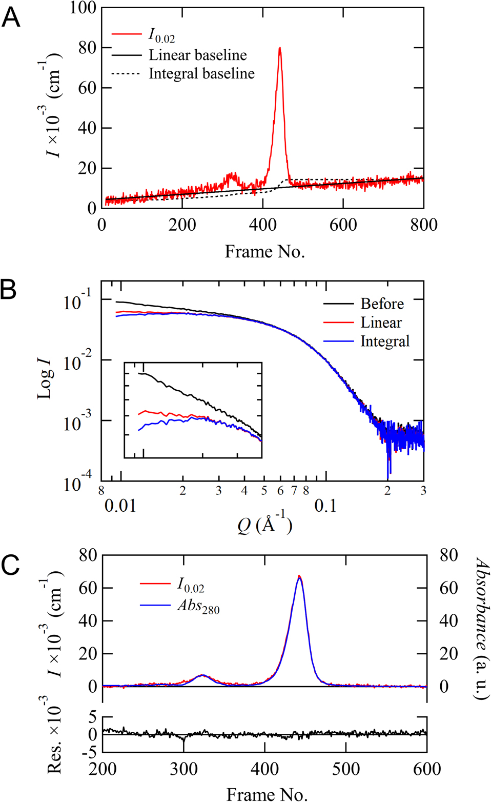
First, we confirmed the accuracy of the baseline correction and mapping optimization functions using SEC-SAXS data of ovalbumin. The following processes are automatically calculated by the software for all data regions. Figure 2A shows the correction process for linear and integral baseline corrections for SAXS data. This figure displays the chromatogram for I0.02 monitored by SEC-SAXS and the corrected baselines. In this case, the linear correction seems to be a better fit than the integral correction. A comparison of the scattering profiles for the main peak (Log I vs. Log Q) before and after the correction is shown in Figure 2B. The scattering intensities in the low Q region after the correction were clearly improved compared to that before the correction. However, the slope of the corrected data is almost zero in the small-angle region for the linear correction, whereas that is slightly decreasing toward the zero-angle for the integral correction. Hence, this result suggests that the linear correction is more appropriate in this case because the integral correction is over-subtracted. Figure 2C shows the final mapping results for the chromatograms for I0.02 and the scaled Abs280. After iteration of both the linear baseline correction and mapping optimization, the residuals between I0.02 and the scaled Abs280 approached zero, as shown at the bottom of Figure 2C. These results indicate that the corrected data set is optimized for subsequent analysis. As the chromatogram in Figure 2C also shows, this ovalbumin solution contains a dimeric component apart from the main monomeric component, successfully analyzing the monomeric component by excluding the dimeric component with gel filtration.
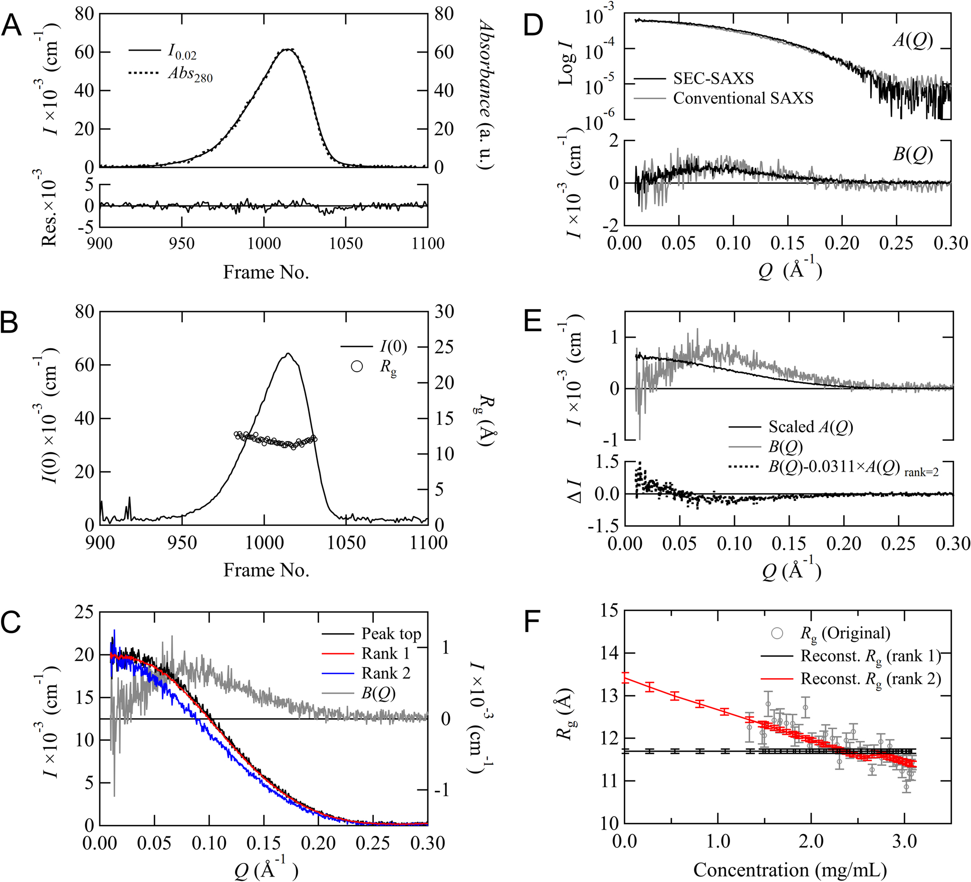
MOLASS has a function that evaluates the effect of concentration dependence on the scattering profiles and automatically removes this effect from the scattering profile to allow for the extraction of only the form factor. That is, this function derives the scattering profile extrapolated to the infinite dilution condition. We confirmed that derivation of the form factor is successfully performed using the rank determination described in Materials and Methods. The SEC-SAXS data of cytochrome C are shown in Figure 3. The chromatograms for I0.02 and Abs280 are plotted in Figure 3A, showing that the baseline correction and the mapping optimization for two data were performed properly. Although the chromatogram for I(0) in Figure 3B depicts a single peak, the superimposed Rg distribution exhibits a slightly convex downward slope. This feature suggests that the data surrounding the peak region are influenced by concentration-dependent effects from interparticle interference. The form factors calculated with rank=1 and rank=2 and the scattering profile for the peak are plotted in Figure 3C. The form factor for rank=1 and the scattering profile for the peak are almost superimposable, but the form factor for rank=2 is different. For rank=2, the component dependent on the concentration is successfully calculated by an extrapolation process that is based on matrix optimization. This concentration-dependent term also appeared when measured with the conventional method shown in Figure 3D, being almost identical to B(Q) in SEC-SAXS. Figure 3E shows that Equation (6) does not converge to zero because the profile shape of B(Q) is different from that of A(Q) by scaling A(Q) to B(Q). Hence, MOLASS determined the rank as 2. We can also confirm that our rank determination process is appropriate by monitoring the concentration dependence of Rg. The Rg values obtained from the Guinier analysis are plotted against the concentrations evaluated using Abs280 (Figure 3F). The Rg values appear to increase linearly toward a concentration of zero. The concentration dependence calculated with rank=1 is different from that of the experimental data, but the dependence calculated with rank=2 overlaps with that of the experimental data. These analyses suggest that concentration-dependent components need to be taken into account when analyzing this data around the peak regions.
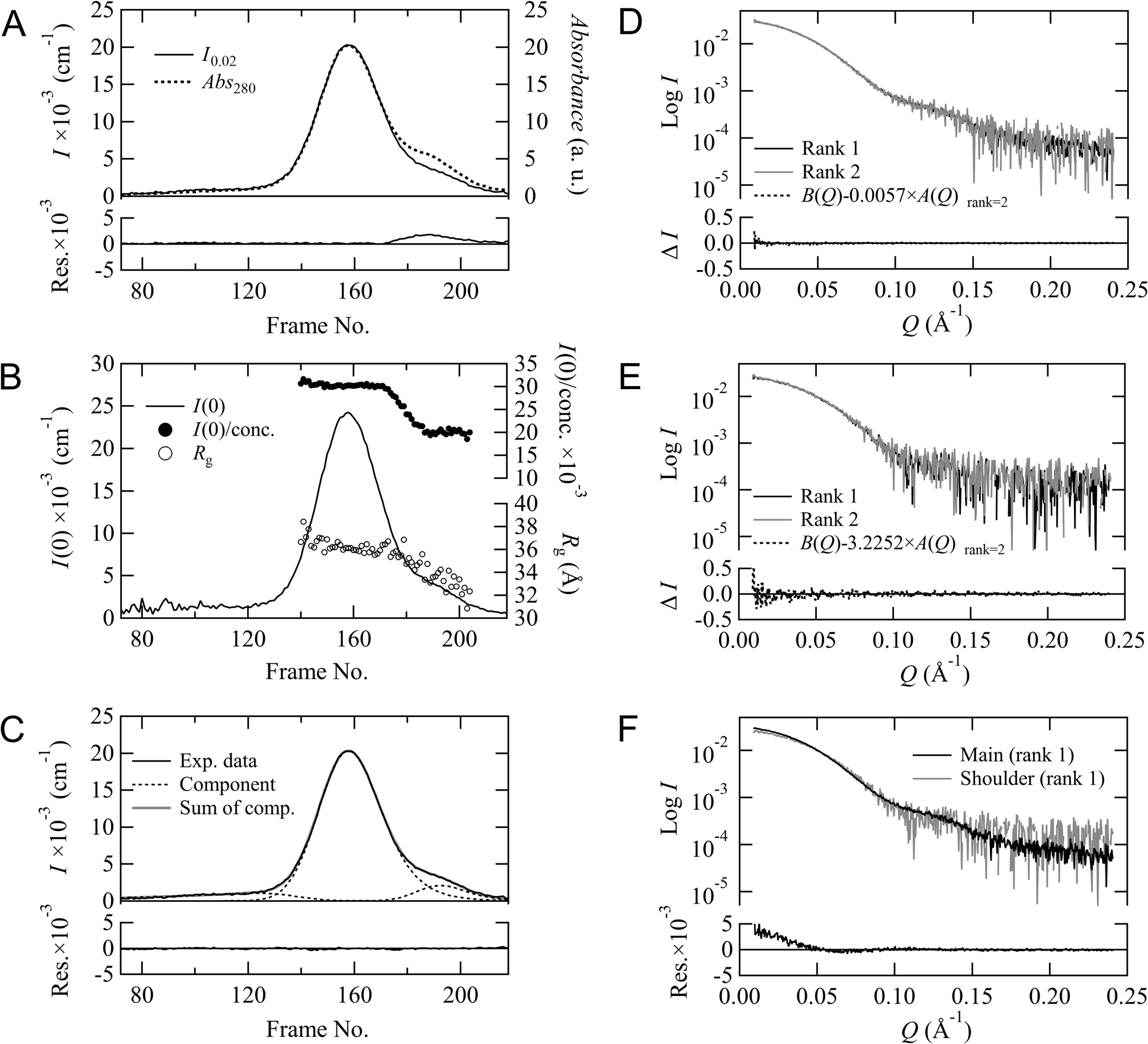
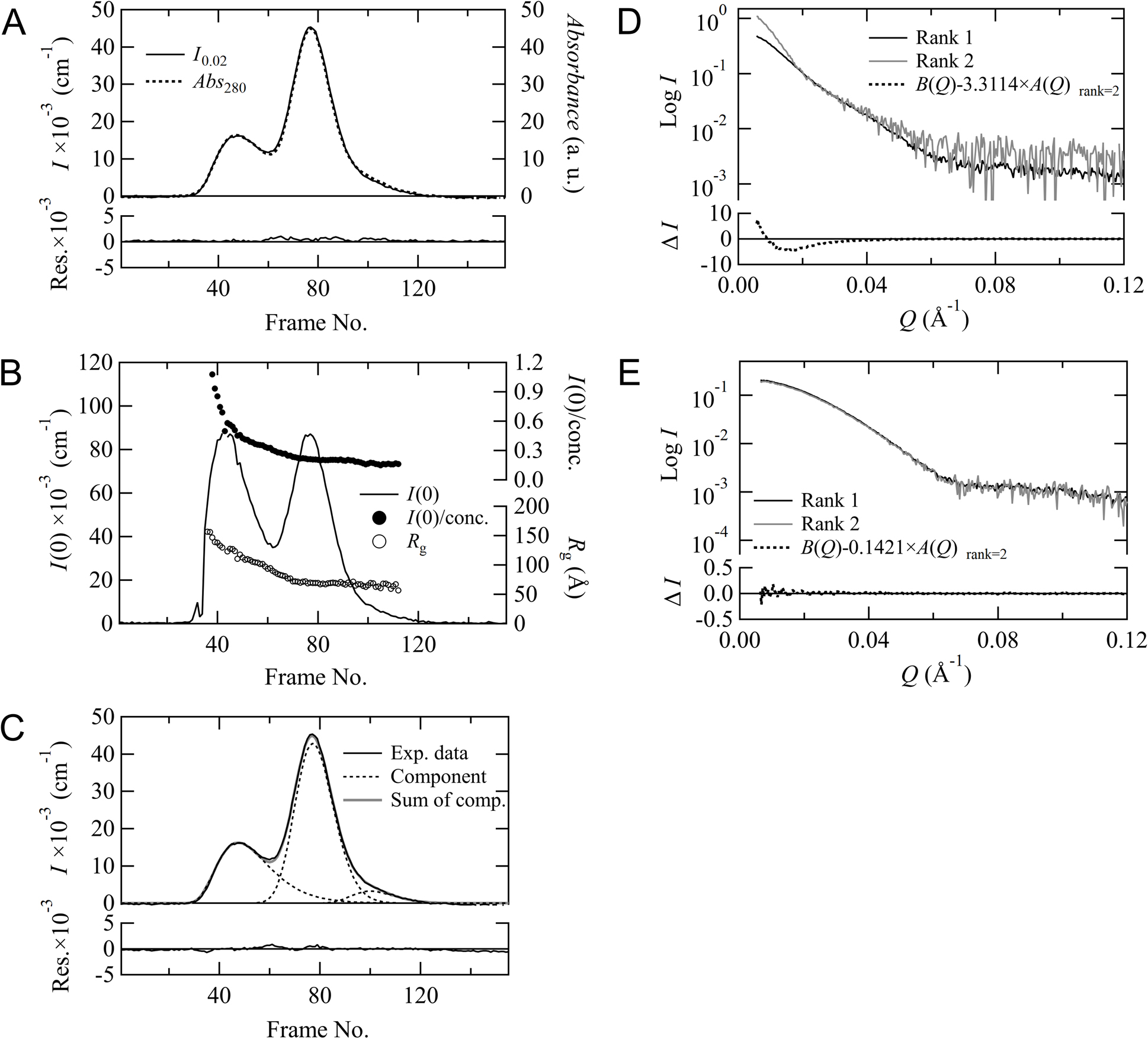
In order to confirm the status of peak decomposition with MOLASS, we analyzed SEC-SAXS data of aldolase. The chromatograms for I0.02 and Abs280 are plotted in Figure 4A, and these elution curves have a shoulder on the descent side of the main peak. We can presume from the residuals displayed at the bottom of Figure 4A that the shoulder region contains another component in addition to the main component. These two components can also be visualized by plotting the Rg values and the I(0)/concentration values obtained from the Guinier analysis (Figure 4B). Peak decomposition analysis was carried out to separate this sub-component present in the shoulder region based on the method described in the supplementary information. Figure 4C demonstrates the result of the decomposition analysis, and the three component curves decomposed by the EMG model and the sum of their curves are overlaid on top of the experimental data. The residuals between the sum of the decomposed components and the experimental data are plotted at the bottom of Figure 4C. The residuals converge to zero, indicating that the decomposition of these components using a modified Gaussian model reproduces the experimental results well. The scattering profiles for the main peak (Figure 4D) and the shoulder peak at the descent side (Figure 4E) were constructed using rank=1 and rank=2. Although A(Q) and B(Q) are successfully separated in the rank=2 processes for each peak, the difference profiles obtained by subtracting the scaled A(Q) from B(Q) based on Equation (6) were close to zero in both cases, indicating that B(Q) is identical to A(Q), respectively. This result suggests that each original scattering profile contains only one component (no concentration dependence) and that these data should be analyzed not as rank=2 but rather as rank=1. The scattering profiles of these two components obtained in the rank=1 process are presented in Figure 4F, showing that their profile shapes are different. Hence, the peak decomposition process of MOLASS could successfully separate the major and minor components of aldolase. As for the weak and broad peak at the upstream side of the main peak, although the component was separated as shown in Figure 4C, its concentration was quite low that it was automatically excluded from the derivation process of the scattering profiles in MOLASS.
To further test the peak decomposition capabilities of MOLASS, we analyzed data for thyroglobulin. This data set also contains two overlapping peaks. Figure 5A shows the result from plotting the chromatograms for I0.02 and the scaled Abs280 together with their residuals. The residuals between the scattering intensity and the absorbance approach zero, indicating that we successfully mapped these chromatograms. By contrast, when Rg and the I(0)/concentration values are plotted against the frame numbers, these data have a non-zero slope for the first peak (Figure 5B). However, no change in these values was observed around the second peak. Hence, it was presumed that the first and second peaks are in the polydisperse and monodisperse states, respectively. The results from decomposition fitting using EGH are displayed in Figure 5C. The chromatogram was decomposed into three components, and the residuals between the sum of the decomposed components and the experimental data were negligible, as shown at the bottom of Figure 5C. The scattering profiles for the first and second components were calculated using rank=1 and rank=2, respectively, but the calculation for the third component is omitted because of low concentration. However, the difference profile for the first peak does not converge to zero, as shown at the bottom of Figure 5D. Because the rank for the first peak is estimated to be 3 or higher from the result in Figure 5B, it would be difficult to derive one form factor profile for this region. By contrast, for the second peak, because Figure 5E demonstrates not only that these profiles constructed using rank=1 and rank=2 are almost identical but also that the difference profile based on Equation (6) converges to zero, the component in this region can be successfully described using rank=1. Hence, for this analysis, only the form factor for the second peak could be obtained.
Discussion
SEC-SAXS makes it possible to extract the structural information for the target state from polydisperse solution samples, and this analysis method is now used for BioSAXS worldwide. In fact, the success rate for structural analysis using BioSAXS has been dramatically improved due to the ability to eliminate the presence of other components and aggregates, which have been fatal problems in conventional concentration-variation analysis. As a result, SEC-SAXS has increased the methodological value of SAXS as a structural analysis tool and has been recognized as one of the important methods in integrative structural biology [35,36]. However, several limitations specific to SEC-SAXS have also been identified over the past decade. We enumerated four major issues in the introduction herein. To address these problems, we developed automatic analysis software for SEC-SAXS, MOLASS, which utilizes the basic theory of SAXS and information science techniques. This software is conceptually aimed at realizing fully automatic calculation of the scattering intensity profile for the most suitable final target from a large number of continuously obtained scattering data by users of all levels of expertise without user bias. In order to achieve this goal, the software was developed in such a way that each of these four issues can be solved one by one using a set of criteria in a sequential process. In addition, the use of low-rank factorization, which is proposed for the combination of UV–visible absorption and chromatography analysis, has made it possible to treat more than hundreds of scattering profiles as a single data matrix, resulting in the simplification of each process.
For baseline correction, we combined two methods of correction, linear and integral, and a method for optimizing the base plane, which allows for adjustment of the entire data set. We can determine which baseline correction is most appropriate and select the one that is more suitable depending on the data. For baseline drift in the ovalbumin data set (Figure 2), the linear correction method was more successful. The usefulness of the integral baseline correction is also recognized for some data, but an insufficient number of our data sets require this correction. Therefore, it will be necessary to continue to search for the best selection conditions for this method and further refine it. When concentration dependence is confirmed, as shown in the results for cytochrome C (Figure 3), it is important to eliminate the concentration-dependent term in order to obtain a scattering profile for which ab initio modeling can be performed. We proposed using the SCD value as a new indicator for the concentration-dependent components in the data sets and determined a threshold value to separate the concentration-dependent components from the statistical information. Hence, MOLASS can be used to correct concentration-dependent effects in SEC-SAXS measurements, which is not possible to do with any other SEC-SAXS analysis software available to date. In cases where multiple peaks overlap in a chromatogram, the user can obtain highly accurate structural information about the target molecule by performing an analysis that properly separates each component. The advantage of simultaneous measurement of SEC-SAXS and UV–visible spectroscopy is not only the measurement of concentration information in real-time but also the identification of other minor components in the overlapping peak regions. In other words, by plotting I0.02 and Abs280, it is possible to determine whether multiple components are included by analyzing the differences between values obtained for the target molecule and the minor component (e.g., differences in I(0)/concentration, Rg, or the extinction coefficient). We established the SCI score as an index to identify these differences using different probes. In addition, when multiple components are included in the chromatogram, MOLASS has a function that performs fitting using a modified Gaussian function of EGH and EMG to separate each peak within the chromatogram. This allows us to recognize and separate the small shoulder components at the descent side of the main peak, as shown for aldolase (Figure 4).
All of the above processes are necessary to extract more reliable information from over hundreds of data. However, the difficulty in any analytical process is to set the optimal initial values because the results are likely to be incorrect without them. If a criterion and a method for each process can be established to provide appropriate initial values, the modules for each process can be connected to achieve fully automatic analysis without user bias. Therefore, the implementation of fully automated data processing means not only the achievement of high-throughput analysis but also the establishment of a methodology to obtain highly accurate structural information by identifying optimal analysis parameters without user bias. Software programs for automatic structure analysis are already being developed in many fields [37–42]. In this study, we attempted to apply automated analysis to relatively less-complicated results from a large number of SEC-SAXS data sets. We confirmed that the automated analysis worked well when the peak data consisted of only a single component for the peak, such as for ovalbumin (Figure 2) and cytochrome C (Figure 3) or when the shoulder peaks were clear, such as for aldolase (Figure 4). By contrast, although a peak composed of a single component measured on the downstream side of the chromatogram was successfully analyzed for thyroglobulin (Figure 5), it was difficult to automatically and correctly analyze a component whose size (Rg) continuously changed with elution volume, such as the peak on the upstream side. Hence, it will be necessary to further improve the fully automated processing to the point where information can be accurately extracted even in complex cases in which two or more components overlap unclearly, such as the upstream peak of thyroglobulin. The challenge with the MOLASS module for separating peaks and calculating certain final scattering profiles is to ensure accuracy for both identifications of the boundaries between overlapping peaks and the determination of optimal data regions to be applied in its calculation. One of the ways to solve the former issue might be to analyze the data without identifying the number of components from the beginning. The latter could be achieved by developing an algorithm that automatically selects the regions where the SCD value stabilizes at the minimum value.
It is difficult for users at all levels of experience to judge and determine the optimal analysis parameters when performing SEC-SAXS analysis. It can be very challenging in SEC-SAXS analysis to establish an automated process to identify the optimal parameters and avoid user bias. MOLASS provides users with empirical standard values derived from a large number of data sets, enabling unbiased analysis. In order to further improve the accuracy of automated analysis in the future, it will be necessary to add new algorithms for experimental results that cannot be deconvoluted with the current software and standardize them to allow for appropriate automated analysis. The best approach to solve this problem commonly encountered by SAXS users would be to compile whole SEC-SAXS data sets collected at not only worldwide synchrotron radiation facilities but laboratory SAXS systems into a data bank and find the patterns that determine the best direction of analysis for each data feature.
Conflict of Interest
All authors declare that they have no conflict of interest.
Author Contributions
K. Yonezawa and N. S. designed this research and conceived the project. K. Yonezawa and M. T. and N. S. analyzed all the data for this manuscript. M. T. developed the source code. All the member discussed the development of software. K. Yonezawa and N. S. wrote the paper.
Data Availability
The evidence data generated and/or analyzed during the current study are available from the corresponding author on reasonable request. The software MOLASS, including its source code, tutorial data and manuals are available from http://pfwww.kek.jp/saxs/MOLASS.html.
Acknowledgements
This research was partially supported by the Platform Project for Supporting Drug Discovery and Life Science Research [Basis for Supporting Innovative Drug Discovery and Life Science Research (BINDS)] from AMED under grant numbers JP21am0101071 and JP22ama121001. This work was also supported by JSPS KAKENHI, grant numbers JP19K06516 and JP19H05781.
References
- [1] Trewhella, J., Duff, A. P., Durand, D., Gabel, F., Guss, J. M., Hendrickson, W. A., et al. 2017 publication guidelines for structural modelling of small-angle scattering data from biomolecules in solution: An update. Acta Crystallogr. Sect. D Struct. Biol. 73, 710–728 (2017). https://doi.org/10.1107/S2059798317011597
- [2] Mathew, E., Mirza, A., Menhart, N. Liquid-chromatography-coupled SAXS for accurate sizing of aggregating proteins. J. Synchrotron Radiat. 11, 314–318 (2004). https://doi.org/10.1107/S0909049504014086
- [3] Ryan, T. M., Trewhella, J., Murphy, J. M., Keown, J. R., Casey, L., Pearce, F. G., et al. An optimized SEC-SAXS system enabling high X-ray dose for rapid SAXS assessment with correlated UV measurements for biomolecular structure analysis. J. Appl. Crystallogr. 51, 97–111 (2018). https://doi.org/10.1107/S1600576717017101
- [4] West, A. L., Evans, S. E., González, J. M., Carter, L. G., Tsuruta, H., Pozharski, E., et al. Ni(II) coordination to mixed sites modulates DNA binding of HpNikR via a long-range effect. Proc. Natl. Acad. Sci. U.S.A. 109, 5633–5638 (2012). https://doi.org/10.1073/pnas.1120283109
- [5] Blanchet, C. E., Spilotros, A., Schwemmer, F., Graewert, M. A., Kikhney, A., Jeffries, C. M., et al. Versatile sample environments and automation for biological solution X-ray scattering experiments at the P12 beamline (PETRA III, DESY). J. Appl. Crystallogr. 48, 431–443 (2015). https://doi.org/10.1107/S160057671500254X
- [6] Cowieson, N. P., Edwards-Gayle, C. J. C., Inoue, K., Khunti, N. S., Doutch, J., Williams, E., et al. Beamline B21: High-throughput small-angle X-ray scattering at Diamond Light Source. J. Synchrotron Radiat. 27, 1438–1446 (2020). https://doi.org/10.1107/S1600577520009960
- [7] Chaudhuri, B., Muñoz, I. G., Qian, S., Urban, V. S. Biological Small Angle Scattering: Tequniques, Strategies and Tips. Advances in Experimental Medicine and Biology vol. 1009 (Springer, Singapore, 2017). https://doi.org/10.1007/978-981-10-6038-0
- [8] Franke, D., Petoukhov, M. V., Konarev, P. V., Panjkovich, A., Tuukkanen, A., Mertens, H. D. T., et al. ATSAS 2.8: A comprehensive data analysis suite for small-angle scattering from macromolecular solutions. J. Appl. Crystallogr. 50, 1212–1225 (2017). https://doi.org/10.1107/S1600576717007786
- [9] Panjkovich, A., Svergun, D. I. CHROMIXS: Automatic and interactive analysis of chromatography-coupled small-angle X-ray scattering data. Bioinformatics 34, 1944–1946 (2018). https://doi.org/10.1093/bioinformatics/btx846
- [10] Manalastas-Cantos, K., Konarev, P. V., Hajizadeh, N. R., Kikhney, A. G., Petoukhov, M. V., Molodenskiy, D. S., et al. ATSAS 3.0 : Expanded functionality and new tools for small-angle scattering data analysis. J. Appl. Crystallogr. 54, 343–355 (2021). https://doi.org/10.1107/s1600576720013412
- [11] Shkumatov, A. V., Strelkov, S. V. DATASW, a tool for HPLC-SAXS data analysis. Acta Crystallogr. Sect. D Biol. Crystallogr. 71, 1347–1350 (2015). https://doi.org/10.1107/S1399004715007154
- [12] Malaby, A. W., Chakravarthy, S., Irving, T. C., Kathuria, S. V., Bilsel, O., Lambright, D. G. Methods for analysis of size-exclusion chromatography-small-angle X-ray scattering and reconstruction of protein scattering. J. Appl. Crystallogr. 48, 1102–1113 (2015). https://doi.org/10.1107/S1600576715010420
- [13] Brookes, E., Vachette, P., Rocco, M., Pérez, J. US-SOMO HPLC-SAXS module: Dealing with capillary fouling and extraction of pure component patterns from poorly resolved SEC-SAXS data. J. Appl. Crystallogr. 49, 1827–1841 (2016). https://doi.org/10.1107/S1600576716011201
- [14] Brookes, E., Pérez, J., Cardinali, B., Profumo, A., Vachette, P., Rocco, M. Fibrinogen species as resolved by HPLC-SAXS data processing within the UltraScan Solution Modeler (US-SOMO) enhanced SAS module. J. Appl. Crystallogr. 46, 1823–1833 (2013). https://doi.org/10.1107/S0021889813027751
- [15] Di Marco, V. B., Bombi, G. G. Mathematical functions for the representation of chromatographic peaks. J. Chromatogr. A 931, 1–30 (2001). https://doi.org/10.1016/S0021-9673(01)01136-0
- [16] Pápai, Z., Pap, T. L. Analysis of peak asymmetry in chromatography. J. Chromatogr. A 953, 31–38 (2002). https://doi.org/10.1016/S0021-9673(02)00121-8
- [17] Maeder, M., Zilian, A. Evolving factor analysis, a new multivariate technique in chromatography. Chemom. Intell. Lab. Syst. 3, 205–213 (1988). https://doi.org/10.1016/0169-7439(88)80051-0
- [18] Meisburger, S. P., Taylor, A. B., Khan, C. A., Zhang, S., Fitzpatrick, P. F., Ando, N. Domain movements upon activation of phenylalanine hydroxylase characterized by crystallography and chromatography-coupled small-angle X-ray scattering. J. Am. Chem. Soc. 138, 6506–6516 (2016). https://doi.org/10.1021/jacs.6b01563
- [19] Nielsen, S. S., Toft, K. N., Snakenborg, D., Jeppesen, M. G., Jacobsen, J. K., Vestergaard, B., et al. BioXTAS RAW, a software program for high-throughput automated small-angle X-ray scattering data reduction and preliminary analysis. J. Appl. Crystallogr. 42, 959–964 (2009). https://doi.org/10.1107/S0021889809023863
- [20] Hopkins, J. B., Gillilan, R. E., Skou, S. BioXTAS RAW: Improvements to a free open-source program for small-angle X-ray scattering data reduction and analysis. J. Appl. Crystallogr. 50, 1545–1553 (2017). https://doi.org/10.1107/S1600576717011438
- [21] Konarev, P. V., Graewert, M. A., Jeffries, C. M., Fukuda, M., Cheremnykh, T. A., Volkov, V. V., et al. EFAMIX, a tool to decompose inline chromatography SAXS data from partially overlapping components. Protein Sci. 31, 269–282 (2022). https://doi.org/10.1002/pro.4237
- [22] Bernadó, P., Shimizu, N., Zaccai, G., Kamikubo, H., Sugiyama, M. Solution scattering approaches to dynamical ordering in biomolecular systems. Biochim. Biophys. Acta Gen. Subj. 1862, 253–274 (2018). https://doi.org/10.1016/j.bbagen.2017.10.015
- [23] Zhang, F., Skoda, M. W. A., Jacobs, R. M. J., Martin, R. A., Martin, C. M., Schreiber, F. Protein interactions studied by SAXS: Effect of ionic strength and protein concentration for BSA in aqueous solutions. J. Phys. Chem. B 111, 251–259 (2007). https://doi.org/10.1021/jp0649955
- [24] Yonezawa, K., Takahashi, M., Yatabe, K., Nagatani, Y., Shimizu, N. Software for serial data analysis measured by SEC-SAXS/UV-Vis spectroscopy. AIP Conf. Proc. 2054, 060082 (2019). https://doi.org/10.1063/1.5084713
- [25] Gasteiger, E., Hoogland, C., Gattiker, A., Duvaud, S., Wilkins, M. R., Appel, R. D., et al. Protein identification and analysis tools on the ExPASy server. Proteomics Protoc. Handb. 571–607 (2005). https://doi.org/10.1385/1592598900
- [26] Petoukhov, M. V., Konarev, P. V., Kikhney, A. G., Svergun, D. I. ATSAS 2.1 - Towards automated and web-supported small-angle scattering data analysis. J. Appl. Crystallogr. 40, 223–228 (2007). https://doi.org/10.1107/S0021889807002853
- [27] Franke, D., Kikhney, A. G., Svergun, D. I. Automated acquisition and analysis of small angle X-ray scattering data. Nucl. Instrum. Methods Phys. Res. A 689, 52–59 (2012). https://doi.org/10.1016/j.nima.2012.06.008
- [28] Grant, T. D. Ab initio electron density determination directly from solution scattering data. Nat. Methods 15, 191–193 (2018). https://doi.org/10.1038/nmeth.4581
- [29] Rüdt, M., Andris, S., Schiemer, R., Hubbuch, J. Factorization of preparative protein chromatograms with hard-constraint multivariate curve resolution and second-derivative pretreatment. J. Chromatogr. A 1585, 152–160 (2019). https://doi.org/10.1016/j.chroma.2018.11.065
- [30] Feigin, L. A., Svergun, D. I. Structure analysis by samll-angle X-ray and neutron scattring (Springer, New York, 1987). https://doi.org/10.1007/978-1-4757-6624-0
- [31] Penrose, R., Todd, J. A. On best approximate solutions of linear matrix equations. Proc. Cambridge Philos. Soc. 52, 17–19 (1956). https://doi.org/10.1017/S0305004100030929
- [32] Penrose, R. A generalized inverse for matrices. Proc. Cambridge Philos. Soc. 51, 406–413 (1955). https://doi.org/10.1017/S0305004100030401
- [33] Svergun, D. I., Koch, M. H. J. Small-angle scattering studies of biological macromolecules in solution. Rep. Prog. Phys. 66, 1735–1782 (2003). https://doi.org/10.1088/0034-4885/66/10/R05
- [34] Mertens, H. D. T., Svergun, D. I. Structural characterization of proteins and complexes using small-angle X-ray solution scattering. J. Struct. Biol. 172, 128–141 (2010). https://doi.org/10.1016/j.jsb.2010.06.012
- [35] Rout, M. P., Sali, A. Principles for integrative structural biology studies. Cell 177, 1384–1403 (2019). https://doi.org/10.1016/j.cell.2019.05.016
- [36] Nakamura, H., Kleywegt, G., Burley, S. K., Markley, J. L. Integrative structural biology with hybrid methods. Advances in Experimental Medicine and Biology vol. 1105 (Springer, Singapore, 2018). https://doi.org/10.1007/978-981-13-2200-6
- [37] Suzuki, Y., Hino, H., Kotsugi, M., Ono, K. Automated estimation of materials parameter from X-ray absorption and electron energy-loss spectra with similarity measures. Npj Comput. Mater. 5, 1–7 (2019). https://doi.org/10.1038/s41524-019-0176-1
- [38] Ozaki, Y., Suzuki, Y., Hawai, T., Saito, K., Onishi, M., Ono, K. Automated crystal structure analysis based on blackbox optimisation. Npj Comput. Mater. 6, 1–7 (2020). https://doi.org/10.1038/s41524-020-0330-9
- [39] Yamashita, K., Hirata, K., Yamamoto, M. KAMO: Towards automated data processing for microcrystals. Acta Crystallogr. Sect. D Struct. Biol. 74, 441–449 (2018). https://doi.org/10.1107/S2059798318004576
- [40] Scheres, S. H. W. RELION: Implementation of a bayesian approach to cryo-EM structure determination. J. Struct. Biol. 180, 519–530 (2012). https://doi.org/10.1016/j.jsb.2012.09.006
- [41] Li, Y., Cash, J. N., Tesmer, J. J. G., Cianfrocco, M. A. High-throughput cryo-EM enabled by user-free preprocessing routines. Structure 28, 858–869.e3 (2020). https://doi.org/10.1016/j.str.2020.03.008
- [42] Stabrin, M., Schoenfeld, F., Wagner, T., Pospich, S., Gatsogiannis, C., Raunser, S. TranSPHIRE: automated and feedback-optimized on-the-fly processing for cryo-EM. Nat. Commun. 11, 1–14 (2020). https://doi.org/10.1038/s41467-020-19513-2

