Measurement of protoplasmic streaming over the entire body of Physarum plasmodium, and estimation of the transport and mixing of protoplasma through the intricate vein network

Abstract

Transport networks spanning the entire body of an organism are key infrastructures for achieving a functional system and facilitating the distribution of nutrients and signals. The large amoeba-like organism Physarum polycephalum has gained attention as a useful model for studying biological transport networks owing to its visible and rapidly adapting vein structure. Using particle-tracking velocimetry, we measured the flow velocity of protoplasmic streaming over the entire body of Physarum plasmodia during the development of its intricate vein network. Based on these measurements, we estimated how the protoplasm is transported and mixed throughout the body. Our findings suggest that the vein network significantly enhances effective mixing of the protoplasm throughout the organism, which may have important physiological implications for nutrient distribution and signaling.

Significance

This study measured the protoplasmic flow within a biological network during the transition from an amorphous state to a developed network. We visualized the spatiotemporal patterns of the flow velocities and conducted a simulation to transport virtual particles based on actual velocity measurements. Our results demonstrated that these particles were well mixed, even in an intracellular viscosity-dominated flow. Our study provides valuable insights into information transfer and morphological transformation within the slime mold network during its development, with potential implications for optimizing artificial transport networks and understanding other biological systems.

 Introduction

Multicellular organisms, including animals, plants, and fungi, form transport networks that span the entire organism. This transport system is indispensable for establishing a body that significantly exceeds the size of a single cell as a functional system. The transport of materials and signals throughout the body is critical for organisms that cannot rely solely on diffusion.

Since around the year 2000, large amoeba-like organism Physarum polycephalum has attracted attention as model organisms for biological transport networks [1–4]. Protoplasmic shuttle streaming has been studied extensively since the 1940s [5]. The Physarum plasmodium has a sheet-like body and forms an intricate network of flow channels (veins) spanning the entire organism. This network can adapt to environmental changes such as the position of food sources by reconstructing itself within a few hours.

When a slime mold escapes from a confined space with a specific geometric shape, it forms a transport network that efficiently discharges its body as reported in previous studies [6]. Recently, there has been an upsurge in experimental and theoretical research aimed at evaluating nonlocal-to-global transport properties related to the topological nature of the vein network [4,7–12]. In particular, Marbach et al. evaluated the effective dispersion throughout a network, defined as the transport capacity [13] and found it to be influenced by changes in the network topology and geometry. They defined effective dispersion as the growth of a cloud of particle dispersion over a long timescale based on local dispersion derived from probabilistic solutions under an advective diffusion system. The study of slime mold networks provides a framework for advancing research on biological transport networks at multiple scales.

Although the functions and capacities of the Physarum network have been studied, experimental measurements of the protoplasmic flow within its network are gaining increasing significance. The scale of measurement has expanded from a single straight strand to veins at a junction [12,14], allowing the examination of the transport and mixing of materials within the network structure. Haupt et al. [12] demonstrated two-dimensional velocity measurements for the flow around the junctions of a network using mPIV (micro-particle Image Velocimetry). They claimed that flow splitting and flow reversal at a junction, as well as the delay in flow reversal in veins at a junction, enhanced the distribution of fluid volume and promoted mixing. Their research was crucial in shaping the methodology of our investigation.

In this study, we employed video image analysis with Particle Tracking Velocimetry (PTV) to measure the flow velocity field across the entire body of a small Physarum specimen. The quasi two-dimensional nature of the plasmodial body allowed for comprehensive imaging and analysis. Although our specimen was smaller than that used by Haupt et al., our analysis encompassed the entire network, thus providing a more complete picture of the organism’s flow dynamics.

We quantified the flow by tracking endogenous microparticles (nuclei, organelles, and starch granules), although the particle density limited the temporal and spatial resolution of our measurements. This approach allowed us to quantify spatiotemporal changes in the flow velocity field during formation of the channel network. Based on these empirical measurements of the flow velocity field, we deterministically simulated the material transport across the body using virtual particles driven sequentially by the observed flow velocity vectors. This simulation visualized the circulation pathways in the cytoplasmic network, providing insights into how materials are exchanged between different local areas.

The transport performance was physically and physiologically characterized before and after the formation of a vein network in Physarum plasmodium. Based on these findings, we explored the mechanism of the mixing and delivery of protoplasm through the vein network.

 Materials and methods

 Organism and culture

The plasmodium of Physarum polycephalum (wild strain) was cultured on a 1% (w/v) agar plate at 25 deg Celsius under dark or dim light, and fed with oats flakes and powders (Quaker Oats Co.) twice a day.

 Chamber for observing the protoplasmic flow and the vein formation

Figure 1 illustrates the experimental setup used to record the development of a vein network from a cytoplasmic droplet under a microscope.

Figure 1  System for measuring protoplasmic flow in the cytosol droplet of the slime mold. (A) Plastic dish (diameter ϕ=150 mm) and (B) the underside of the dish lid. Holes in the shape of a rounded rectangle (A) and a circle (B) were made with a drill and a rectangular cover glasses was glued with resin. The cytosol droplet (green ellipse) is covered with a sheet of agar (blue rectangle). Figure 1(C) The dish and lid are piled up on the stage of an upright microscope (UMS). The edge of the lid was removed to allow lens focus adjustment, and 4 small dishes (ϕ=35 mm) were used as supports. Wet papers were put around the space around the dishes and a siphon was inserted through an indentation in the lid edge. The specimen was illuminated from below with red light, and focused on through 10x objective lens, by focusing on the cortex near the substrate side, and captured with CMOS camera (Orca spark).

To maintain optimal observation conditions for video recording for several hours, we prepared a custom-made chamber (Figure 1A, B). The biological specimen was placed at the center of a plastic chamber (Petri dish and lid). The central part of the plastic chamber (both the lid and container) was replaced with a thin transparent glass plate (cover glass) with good optical properties to ensure that the specimen image was well resolved (Figure 1A~C).

Wet paper was placed inside the chamber to prevent the specimens from drying. Water was supplied at a controlled rate from a reservoir positioned slightly higher than that of the wet paper using a siphon. To prevent fogging of the cover glass window, excess humidity in the chamber was reduced via several holes in the chamber wall (Figure 1B). By carefully tuning the humidity, the glass window was kept sufficiently clear to observe the flow of intracellular particles for several hours.

 Preparation of biological specimen for the microscopic measurement

A thick vein of a large plasmodium (approximately 20×30 cm) was cut with a scalpel, causing the protoplasmic sol to leak from the vein. The leaking droplets were quickly collected and placed on a cover glass at the center of the chamber lid for measurement. To prevent the droplet from drying out, we applied a drop of water to the sample and covered it with a thin sheet of agar (approx. 0.1 mm thickness). The lid with the specimen was then placed upside down on a chamber dish positioned on the stage of the UMS (BX-53, Olympus) (Figure 1C).

 Setup of microscopy and video-recording system

To minimize the side effects of the observation light, the specimen was illuminated with red light (wavelength of approximately 700 nm) by filtering out shorter wavelengths from the white light of UMS. The CMOS camera (Orca Spark) attached to the UMS was connected to a computer (GALLERIA, GCF1050TNF) equipped with HD (hard disk, IODATA HDJA-UT8.0W) (Figure 1C). The images originally captured at a resolution of 1024 pixels×1024 pixels were binned to 512 pixels×512 pixels to conserve memory volume during analysis (with a pixel resolution of 2.3 μm×2.3 μm at 10 frames per second (FPS). The camera was set to the following parameters: exposure time, 50 ms; gain 0, and binning, 0. Because of the memory limitation of the recording system, image recording was conducted for 30-minute time windows, with repetitions occurring with a gap of five-minutes between them, for up to 2.5 hours from the start of observation. For convenience, we refer to each 30-minute interval as follows: 30 min (t=30~55 min), 60 min (t=60~85 min), 90 min (t=90~115 min), and 120 min (t=120~145 min). The initial 30 min (t=0~25 min) was excluded from this categorization because the particle tracking (described below) was not functional during this period. The experiment was repeated three times, and we labeled each trial as Exp1, Exp2, and Exp3. For clarity, we present the results of Exp1 as a representative case.

 Image processing for detecting the intrinsic intracellular moving particles

The intensity of each pixel in the captured image I(x, y, t), where x and y represent spatial coordinates and t represents time, was processed to detect the intrinsically moving particles [15]. The difference between the intensity of each pixel and the average intensity over a specified time window (12 s) was calculated and is denoted as ΔI (x, y, t):

  

$$\Delta I(x,y,t)=I(x,y,t)-{\int }_{t-6t}^{t+6fis}I(x,y,t)dt.$$(1)

In this equation, the raw data I represents the captured image, as shown in Figure 2A (captured at t=32 min 37.4 s), and ΔI emphasizes the moving particles, as shown in Figure 2B. This method typically visualizes particles sufficiently clearly for a developed network or a thin, extended cell (for t=60 min and beyond). However, for the thicker cells in the early stages of development (0~60 min), the particles shown in Fig. 2B were not as clear for particle tracking. This highlights the need for further improvements to enhance the visualization in such cases.

Figure 2  Example of image processing. (A) Raw input image I, captured at t=32 min 37.4 s. (B) Processed image ΔI, (C) Phase θ of ΔI, and (D) Time-averaged phase $\overline{𝛉}$ to reduce noise. (E) Detected particles and their trajectories using particle tracking velocimetry (PTV), shown after inverting light intensity of the image. The detected particles are represented by white circles (radius=5 μm) with short black trajectories marking their movement at the center of each circle.

Therefore, we normalized ΔI to obtain the phase θ (x, y, t) of the time-series signal ΔI. The signal was divided into periodic segments by detecting the minima of |ΔI (x, y, t)| and normalizing by the maxima of |ΔI (x, y, t)| within each period of shuttle streaming, a phenomenon linked to periodic changes in cell thickness. The phase θ (x, y, t) is defined as the phase of sin waves of an irregular period and amplitude max(|ΔI (x, y, t)|),

  

$$\theta (x,y,t)={sin}^{-1}(\Delta I(x,y,t)/max\left(\left|\Delta I(x,y,t)\right|\right)).$$(2)

The sin^–1 function emphasizes the differences in values close to –1 or 1 in –1≤ΔI(x,y,t)/max(|ΔI(x,y,t)|)≤1.

The image of θ(x, y, t) was highly sensitive to moving particles, but prone to noise (Fig. 2C). To reduce noise, we computed the time-average over a short-term (Fig. 2D),

  

$$\overline{\theta (x,y,t)}={{\int }_{}^{}}_{t-0.6s}^{t+0.6s}\theta (x,y,t)dt$$(3)

The processed image of $\overline{\theta (x,y,t)}$ was used only for the time interval between 30 and 55 min from the start of the observation. Although the exact composition of these particles could not be definitively determined, they appeared to resemble stacked materials, such as starch granules in vacuoles, based on their observed diameters, which varied from 6 to 30 μm. This diameter range is generally larger than that of nuclei and organelles.

 PTV for measuring the velocity of intrinsic moving particle in the specimen

We employed the TrackMate [16]-free software plugin of Fiji [17] for Particle Tracking Velocimetry (PTV) (Fig. 2E). Trackmate automatically identifies particles based on user-defined criteria, such as particle size and threshold value. To detect the particles in each image, we used the Laplacian of the Gaussian (LoG) tracker, defined as follows:

  

$$Lo{G}_{\sigma }=-{\sigma }^2*(\frac{{\partial }^2}{\partial X^2}+\frac{{\partial }^2}{\partial Y^2})*G_{\sigma }*I$$(4)

$\sigma =R/\sqrt{2}$ where R denotes the particle radius (R=5 pixels ≃11 μm). Initially, TrackMate filters the input test images I using a Gaussian filter G_σ to reduce noise. Then, a Laplacian filter (∂²/∂X²+∂²/∂Y²) is used to detect the particle boundaries. Finally, the filtered images are inverted and normalized using –σ². In these processed images, the values peaked at the center of particles with diameters ranging from 5 to 20 pixels, allowing precise particle localization.

The process of linking particles between successive images occurs in two steps: (1) creating track segments linking particles in consecutive frames and (2) bridging the gap between two track segments. In both steps, TrackMate solve the Linear Assignment problem (LAP). It computes a cost matrix representing the possible linking costs between particles, and determines the optimal assignment by minimizing the total cost. Please see the manual of TrackMate and Fiji in details (https://imagej.net/media/plugins/trackmate/trackmate-manual.pdf).

Given that the number of intrinsically moving particles passing through a 4×4 pixel area over 10 s was limited to approximately ten particles, we adjusted both the spatial and temporal resolutions for each step of the analysis.

 Extraction of graph structure of flow-Network and flow rate on it

While the plasmodial droplets formed a network, the morphology of the network channels was not easily discernible. To estimate the morphology, we created binary maps from Particle Tracking Velocimetry (PTV) data within Fiji, where data points were aggregated over a 2×2 pixel grid every minute (Figure 3A). We summed the PTV data for each pixel and applied automatic binarization to create a binary mask. Next, using functions from Scikit-image and SciPy in Python, we skeletonized the binary mask to determine the central positions of the network channels. The radius of each channel was calculated as the distance from the skeleton to background. The terminal branches of the skeleton were pruned to simplify the network structure.

Figure 3  Process of construction of the network from the experimental data. (A) The sum of binary maps, where white pixels represent areas where PTV data were detected multiple times within the range of (2 pixels, 2 pixels). This figure represents the cummulative data collected after 120 minutes (121 min~144 min). (B) The graph network of (A) based on result of Analyze Skeletonize in Fiji. (C) The simplified graph of (B) by pruning nodes with 2 edges.

We identified the network nodes (intersections) and edges using the Analyze Skeleton plugin in Fiji [18]. Figure 3(B) shows the flow network. Despite pruning the short branches, some unnecessary nodes with only two edges remain (Figure 3B). We further prune these nodes and reconnect the remaining nodes to produce the final simplified network, as shown in Figure 3C.

To calculate the speed profiles at each position on the skeleton, we generated Mean Flow Velocity (MeanFV) maps. These maps were computed by averaging the velocity of PTV data within windows of (±4 pixels, ±4 pixels, ±5 seconds) for each pixel every second. In other words, MeanFV was updated in one second but it was a moving average over ±5 seconds. The direction of the speed profiles was estimated along the axis perpendicular to the local skeleton direction, and the profile width was extended to both sides of the skeleton up to a known channel radius.

The flow rate Q of the speed profile was calculated $Q={\int }_0^{2\pi }{\int }_0^{r_0}v(r,\theta )drd\theta$ from the measured velocity profile v(r)[0≤r≤r₀] along the radius r₀ of the flow channel. The mean speed $\bar{v}$ was determined by dividing the flow rate Q by the circular channel cross-sectional area. Finally, the values for each edge of the network were averaged.

 Estimation of mass transport rate and its energy efficiency

To evaluate the transport efficiency of the network, we estimated the protoplasm transport rate and its associated energy cost, which are basic indicators of flow network performance. We modeled the protoplasmic flow using the Hagen-Poiseuille equation (Q=d·Δp), where Q is the volumetric flow rate, Δp is the pressure difference between two points separated by distance L, and d is the conductivity given by $d=\frac{\pi r^4}{8\eta L}$. Here, r is the radius of the flow channel and η is the viscosity of the endoplasm, assumed to be 2.0×10^–3 Pa·s [12]. We defined the Mass Transport Rate (MTR) as the line integral of the mass flow rate along the network as MTR=∫ρ|Q|ds, where ρ is the density of the protoplasm, taken as 1120 kg/m³ [12], and ds is line segment. To quantify the energy expenditure, we calculated the Work Expenditure (WE): WE=∫|Q|·|∇p|ds=∫8ηQ²/(πr⁴)ds, where |∇p| is the pressure gradient (|∇p|=Δp/L=|Q|·8η/πr⁴). Finally, we defined transport efficiency as the ratio of MTR to WE: Transport Efficiency=$\frac{MTR}{WE}$. This ratio provides a measure of the mass transported per unit of energy expended, allowing for an assessment of the overall performance of the protoplasmic transport network.

 Results of biological experiment

 Development of network of flow channels in the plasmodial droplet

Figures 4A–D show snapshots of the plasmodial protoplasmic droplets over time. Within 30 min of droplet setup (A), rhythmic deformation and cytoplasmic streaming were gradually initiated. As the process progressed, the droplets began to spread and became thinner (B). Simultaneously, flow channels for protoplasmic streaming emerged. These channels continue to develop, eventually forming a complex network of interconnected channels with varying diameters throughout the plasmodial droplets (C, D).

Figure 4  Images of plasmodial droplet (Exp1) at 44 min 20 sec (A), 74 min 20 sec (B), 104 min 20 sec (C), and 134 min 20 sec (D) after the preparation of the plasmodial droplet. Two-dimensional maps of MaxFS during 1 minutes are shown at at 39 min 20 sec (A’), 69 min 20 sec (B’), 99 min 20 sec (C’), and 129 min 20 sec (D’) after preparation. (E) Time course of MaxFS along the pink line in figure A’ on the specimen. The one-dimensional space from left to right in Fig. A’ is indicated from top to down in Figure E. Results of Exp2 after 123 min are shown in (F) and (F’), and Exp3 after 142 min are in (G) and (G’). Scale bar: 250 μm. The maximum flow speed at each element was calculated in a window of (2 pixels×2 pixels ≃4 μm×4 μm) over one minute.

Figures 4A’–D’ illustrate the spatial map of the maximum flow speed (MaxFS) over a 1-minute interval (the maximum speed during a complete cycle of protoplasmic shuttle streaming) at each position within the plasmodial droplet and are depicted using a color chart. Initially (A’), MaxFS is low (dark blue). As the droplet spreads and thins, a high-speed channel forms (B’). Over time, some of these channels thicken, whereas others disappear. Generally, larger channel diameters correspond to a faster MaxFS (C’, D’). Once the channel network was fully developed, a thick annular channel appeared in the central region of the droplet, referred to as the central annular channel (CAC).

Figures 4E illustrates the time course of flow speed along the horizontal line (pink line in Figure 4A’). The CAC opened quickly for approximately 90 min, as shown in Figure 4E. A channel network is systematically constructed throughout the plasmodial droplets. Similar CAC formations were observed in Exp 2 (F, F’) and Exp3 (G, G’) as well. A quantitative analysis of the shape and transport functions of this channel network is necessary for the next stage of the study.

 Development of spatio-temporal patterns of shuttle flow through the central thick annular channel of transport network

Figure 5 illustrates the typical spatiotemporal pattern of the protoplasmic flow at each 30-minute interval. This figure represents the MeanFV map of a plasmodial droplet. Each row was arranged in 20-second step, and vertically aligned within each 30-minute term. The flow direction reverses approximately every 40 s, resulting in a shuttle flow throughout the entire area. By 90–120 min, the central annular channel (CAC) was fully established.

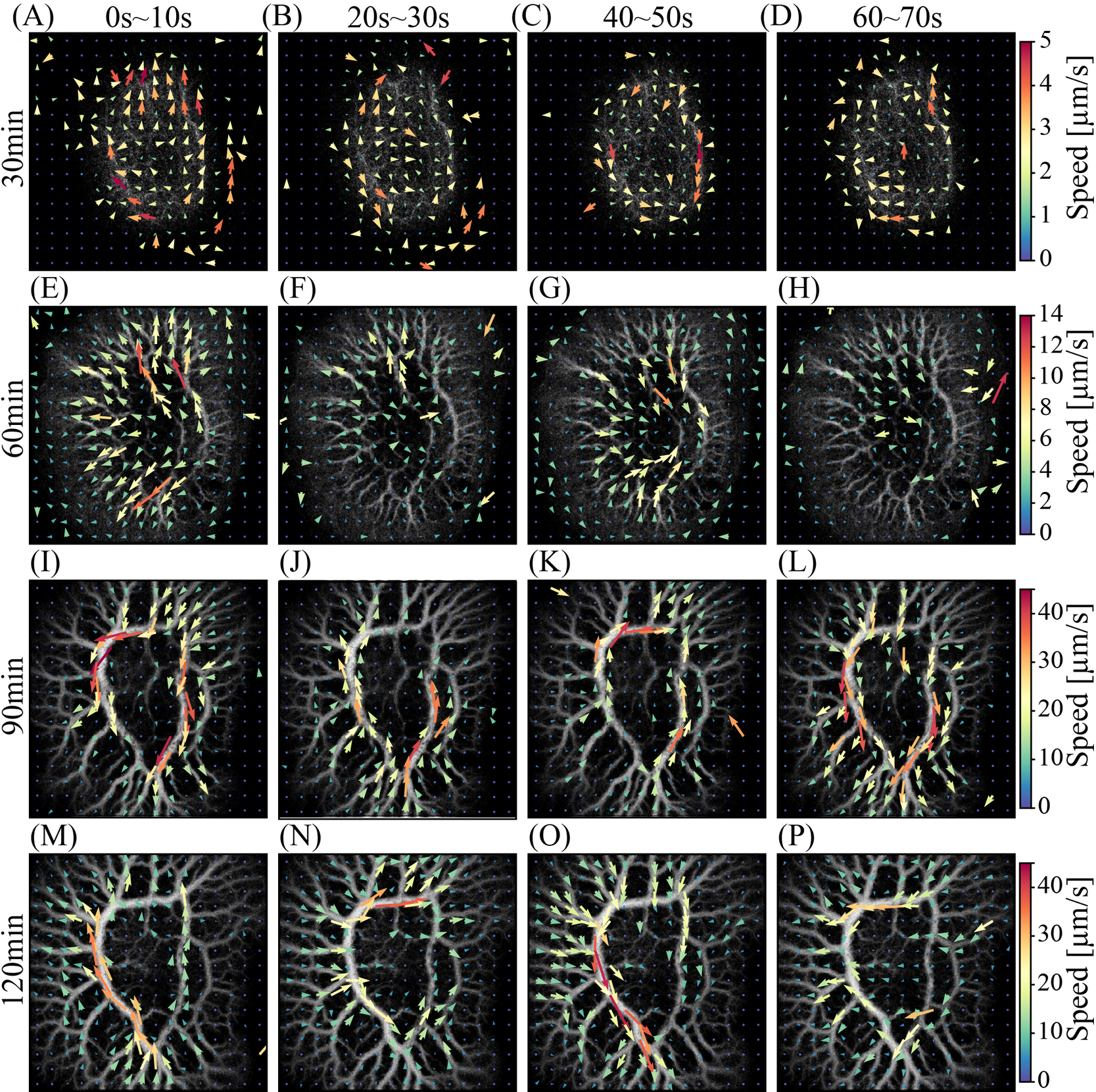
Figure 5  Two-dimensional patterns of MeanFV at various times after the preparation of the plasmodial droplet. For the sake of visual recognition, these figures are shown at a spatial resolution (averaged over ±16 pixels×±16 pixels) lower than that of the actual data obtained (avegraged over ±4 pixels×±4 pixels). Each row represents four patterns obtained successively every 20 seconds, illustrating the periodic switching (approximately 40 seconds) of flow direction. The vertical arrangement of each row indicates the time sequence at 30-minute intervals following droplet preparation.

For example, in Figure 5M, the flow converges to the CAC from the narrow channels in the lower region of the figure. The flow then accelerated along the CAC and exited toward the narrow channels in the upper-left region, suggesting that intracellular materials such as vesicles and particles could be transported from the lower to the upper-left region.

In Figure 5O, 40 seconds after Figure 5M, the flow vectors were, roughly speaking, reversed compared to the previous configuration. Consequently, intracellular materials can be transported from the upper-left region to the lower one. This suggests that intracellular substances are delivered alternately between distant locations within the plasmodial body via the CAC.

Next, we reduced the flow pattern to a simpler representation of transport by extracting the graph structure, as shown in Figure 6. The edges represent the flow direction and rate, as indicated by the arrows and colors, respectively. There are two types of triple-junction nodes: convergence (two inlets and one outlet, represented by red dots) and divergence (one inlet and two outlets, represented by blue dots). Divergence nodes play a crucial role in matter diffusion as noted by Haupt et al. [12].

Figure 6  Graph representation of the flow pattern. The network of flow channels has been simplified into a graph consisting of nodes and edges. Arrows on the edges indicate the direction of flow, while the color represents the flow rate, larger flow rates are depicted in orange, and lower flow rates in pale greenish-yellow. Nodes are categorized into divergence nodes (blue circles, one inlet and two outlets) and convergence nodes (red circles, two inlets and one outlet). The CAC of the flow network is indicated by green lines, while other channels are represented by white lines. (A) t=132 min 40 sec, (B) t=132 min 40 sec.

In Figure 6A, the flow in the top-right area tends to be directed toward the CAC via a cluster of convergence nodes, whereas the flow in the left half is directed from the CAC to the periphery through the divergence nodes. These flow directions are reversed after approximately 40 s (B). At this point, most divergent nodes switch to convergent nodes, and vice versa. In this manner, the particles move back and forth through these nodes. Measuring the delivery and mixing of particles throughout the plasmodial body is of great interest; however, tracking individual particles over an extended period presents challenges. Therefore, we propose a theoretical estimation method using a simulation of virtual particles based on the real velocity field measured in this experiment.

 Increase of mass transport and estimation of mass transport by unit cost

To evaluate network performance over time, we analyzed the Mass Transport Rate (MTR) and Work Expenditure (WE) across the entire network assuming Hagen-Poiseuille flow conditions. Figure 7A illustrates the time courses of MTR and WE over the network. The MTR increased by more than ten times, from less than 0.02×10^–12 [kg·m/s] (30~50 min) to over 0.3×10^–12 [kg·m/s] (120~140 min). Concurrently, WE also increased as the channel network developed. In Exp1 and Exp2, both MTR and WE increased prominently after 90 min, coinciding with the transformation into a protoplasmic network. Whereas for Exp3, this increase occurred after 120 min. Ultimately, as the network structure stabilized, both MTR and WE converged to similar values across all three samples.

Figure 7  Time courses of (A) Mass Transport Rate (MTR) (gray symbols) and Work Expenditure (WE) (white symbols) across the network, assuming Hagen-Poisueille flow, and (B) the ratio of MTR to WE (MTR/WE). Different shapes represent each experiment: circle (Exp1), square (Exp2) and triangle (Exp3). Each symbol represents values averaged over a moving window of ±60 seconds, plotted at 5-minute intervals. As the channel network developed and organized, both the mass transport rate and work expenditure increased significantly, while the mass transport per unit work expenditure showed only a slight decrease.

Figure 7B shows the time course of the ratio MTR/WE, which represents the transport efficiency. Initially (30–50 min), this ratio was similar across the experiments, ranging from 1 to 2. After the transient increases between 90–120 minutes, it converged to approximately 1.3 around 120–140 minutes. Notably, although the mass transport rate increased significantly with network development, the MTR/WE ratio remained relatively stable.

 Simulated estimation of material transport and mixing, based on the measured flow vector field of flow

 Simulation methodology

We conducted simulations based on the measured flow velocity field data to further investigate the dynamics of material movement within the network.

We simulated the transport of virtual particles using the measured mean flow velocity (MeanFV) field. Particle trajectories were traced by integrating the flow velocity from the initial positions at 0.1-second time steps, up to 500 s, while MeanFV was updated in one second. In each simulation, 15 virtual particles were placed at slightly different initial positions within the local region of the cell body. This simulation was repeated at least 16 times from various initial regions across the entire cell body, and the number of repeats was 16, 29, 19, and 26 for 30, 60, 90, and 120 min, respectively; therefore, the total number of trajectories of the virtual particles calculated statistically was 240, 435, 285, and 390, respectively.

It is important to note that our simulation neglects particle diffusion due to thermal fluctuations, which become significant when the particle speed from advection is low. We derived the conditions under which diffusion was negligible compared to advection. For a tube of length ℓ, the time taken for a particle to traverse from one end to the other by diffusion is given by: ℓ²/(2D_T), where D_T is a diffusion constant, and Taylor’s dispersion is neglected for simplicity. In contrast, the time taken by advection is ℓ/v, where v is the particle speed. Therefore, the condition is expressed as ℓ²/(2D_T)>>ℓ/v. When we rewrite this equation using the Einstein-Stokes relation D_T=kT/6πηℓa, we obtain

  

$$a\gg \frac{kT}{3\pi \eta 𝓁v},$$(5)

where a denotes the radius of the particles, k=1.38×10²³ JK^–1 denotes the Boltzmann constant, and T=293K denotes the temperature. This inequality indicates that our simulation is valid for particles with radii larger than that on the right-hand side.

The maximum and minimum values on the right-hand side of Eq. 5 are, respectively, 11 nm and 0.09 nm, which are calculated from ℓ=10 μm and v=2 μm/s and from ℓ=120 μm and v=20 μm/s (these values were obtained from Results of Simulation: Quantitative Estimation for Transport), where we have assumed that η=0.002 Pa s. The latter can also be applied to single macromolecules. The internal vesicles observed in this study are larger than 1 μm. Therefore, inequality 5 is satisfied.

 Estimation of transport capacity of the network

To evaluate the transport capacity of the network, we calculated the mean square displacement MSD between the initial and present positions of all particles in all simulations. Although in advection-dominated systems, particle displacement is typically thought to be proportional to time, that is, MSD is proportional to the square of time, a diffusive property, MSD∝t, can be expected to appear in our system. In fact, as shown in Figure 9, MSD increases linearly with a small oscillation caused by the shuttle flow. The diffusion constant D was obtained by fitting a straight line using the least squares method over a sufficiently long timescale T (until the third minimum in MSD). Because our system is two-dimensional, we can relate the diffusion constant to the slope of the fitting line as D=α/4, where α represents the slope of the fitting line.

Figure 9  Transport distance of virtual particles, simulated from the various initial local regions and diffusion constant D. (A) The solid black line represents the average of mean square displacement (MSD), with the black dot indicating the local minimum of MSD. The grey solid line is the fitting line for the first three black dots and the origin obtained by the least-square method, represented by the equation MSD=4Dt, where D is the diffusion constant and t is time. The white circle with error bar shows the average $⟨\mathbf{\sum }{\overrightarrow{\mathit{r}}}_{𝐢}^{\mathrm{𝟐}}⟩$ with the standard error. Additionally, we measured the spreading of particle by calculating the mean number of nodes that a particle traversed, indicated by the gray dashed line (divergence nodes) and black dotted line (convergence nodes). (B) Time course of mean length d between divergence nodes (gray symbols) and mean speed v (white symbols) of a particle across all simulations. Both values increased significantly after 90 minutes, coinciding with network development. (C) Time course of diffusion constant D (gray) and dv/4 (white). The diffusion constant D increased as the network matured. The shapes of the symbols vary for each experiment: circle (Exp1), square (Exp2), and triangle (Exp3).

To further quantify the dispersion capacity of the network, we calculated the area coverage rate (ACR), defined as ACR=(area of the convex envelope for tracks of all scattered particles)/(area of plasmodial droplets).

 Estimation of particle mixing among four compartments

To quantify the mixing of virtual particles, we simulated the simultaneous transport of multiple virtual particles through-out the cell. We divided the space virtually into four quadrants using diagonal lines drawn from the corners of the figure frame (Figure 3A). Within each compartment, we randomly placed 750 virtual particles, each of which was assigned a unique color corresponding to its initial quadrant. To focus on network-driven mixing, we excluded the central annular channels (CAC) from initial particle placement.

 Results of simulation

 Simulation for movement of virtual particles initially given at a specific local region, based on the numerical integration of measured flow vectors

Figure 8C shows the trajectories of 15 virtual particles (red squares) initially placed within a narrow region with a slight shift (within 32 μm×32 μm) and transported from time 0 to 500 s.

Figure 8  MeanFVs of divergent (A) and convergent (B) junctions, along with the simulation of virtual particle transport (C, D). Fifteen virtual particles (red squares) of which their initial positions were slightly different (1 pixel displacement) along a cross section of a thick vein on the CAC (C). Trajectory of each particle was calculated at the time step of 0.1 seconds according to the experimental data of MeanFV updated by a second, each particle’s movement is represented by differently colored lines from time 0. Over time, the virtual particles dispersed throughout the body, moving back and forth from time 0 to 500 seconds. By 100 seconds, the dispersion covered a portion of the organism, reaching the full range by 300 and 500 seconds. A single particle’s path (D) is traced, illustrating its transport through the CAC and migration within a local area of the body.

During one cycle of the protoplasmic shuttle flow at 100 s, these particles passed through the central annular channels (CAC) for some time before moving into narrower channels and subsequently repeating the movement. By 300 seconds, they had spread widely throughout the organism, and by 500 seconds, they had maintained a global distribution across the entire body. Despite their nearly identical initial positions, the final destination sites varied at 500 s, indicating extensive dispersal throughout the organism. The trajectories also differed; however, many were similar when passing through the CAC. These results demonstrated that local materials were effectively delivered to most regions of the body.

Figure 8D illustrates the movement of a single particle. The particle travelled back and forth through CAC, visited a local network of narrow channels, and remained in the area for some time. It then migrated among various remote local regions via the CAC over 500-second duration. This implies that the transport of materials between remote local regions is mediated by the initial flow through the CAC.

Figures 8A and B show the detailed flows at the triple junction of the flow channels as a particle moves in and out of the central annular channels. In the case of a divergent flow pattern from CAC (A), the flow vectors coming from the top right to the junction were not perfectly parallel to the channel; they exhibited fluctuations with some perpendicular components. Consequently, the flowing particles shift along the direction of the channel width before the triple junction. This shift incidentally distributes the stream into two paths at the triple junction: distribution to CAC or a local narrower channel. This inevitable selection of the moving direction at the junction is one of the causes of the stochastic nature of the particle motion.

 Quantitative estimation for transport

In the mature network, after 120 min (Figure 9A), the particles rapidly dispersed to an area of 180000 μm² (=424 μm long) within the first 100 s on an average of 390 trajectories starting from various initial positions throughout the cell body. The particles circulated along the CAC, moving in and out of the CAC due to the flow bifurcations, which caused the MSD to oscillate. Our results indicated that the particles traveled nearly half the length of the cell body within the first 100 s (after one cycle of protoplasmic flow). However, the MSD had saturated at 200 s, owing to constraints imposed by the cell size or because some particles had already reached the edges of the captured area.

On average, the particles passed through approximately 25 divergence nodes (gray dashed line in Figure 9A) and 23 convergence nodes (black dotted line in Figure 9A) in 500 s. This indicates that the average time for the particles to move between two adjacent nodes was approximately 10.4 seconds. This implies that during one cycle of the protoplasmic flow (approximately 80 s), the particles passed through approximately eight nodes (Figure 9A), and particles potentially have approximately four chances to be dispersed at divergence nodes. This passage through the nodes is closely related to the delivery and mixing of materials throughout the body.

Figure 9B shows the average distance d between the divergence nodes and mean speed v of the particles. This mean speed is calculated by dividing the distance between adjacent divergence nodes by the time it takes to move between these nodes and then taking the average. In all the three experimental cases, as the network matured, the mean speed v of the particles increased (white symbols in Fig. 9B).

As a result of this increase in the particle speed, the diffusion constant D of the particle movement increased from very low values at 60 min to a significantly higher level after 90 min, once the CAC structure had fully developed.

 Estimation of planar dispersion of the virtual particles

To observe how the particles spread and covered the body of the organism, we defined the area-coverage rate (ACR) as the ratio of the distribution range of the particles (illustrated by the blue polygon in Fig. 10A–B) to the whole area of body (represented by the black background in Fig. 10A–B). The time course of ACR averaged across all the simulation cases is shown in Fig. 10C. ACR increased linearly with time over the course of 500 seconds. Initially, at 30 and 60 min, ACR remained low, approximately 0.1, but increased to 0.7, once the CAC was fully established between 90 and 120 min. On average, the particles were dispersed to approximately half the area of the organism within 300 s via CAC.

Figure 10  Planar dispersion of virtual particles. (A) and (B) show an examples of simulation of planar dispersion((A) t=0 s, (B) t=500 s). The virtual particles (red squares) and their tracks are the same as those in Fig. 8C. The dark background indicates the full area of the cell, and the area of dispersion is defined as the convex envelop connecting the outermost particles (blue polygon). (C) Time course of the area coverage rate (ACR) of dispersed particles across the whole cell over four different 30 minutes terms (for Exp1). The 4 different patterns of black dashed lines show average of ACR for each term, with gray lines of the same pattern indicating the range of standard deviation. The gray line is the fitting line for the ACR at 120 minutes over the first 200 seconds. (D) Time course of the slope of ACR at each 30 minutes term for three experiments, illustrating how rapidly particles mixed throughout the cell.

The solid grey line in Fig. 10C represents the fitting line for the first 200 seconds of the average ACR at the 120-minute mark. Figure 10D shows the time course of the initial rate of ACR increase in Experiments 1–3. This result demonstrates that the planar dispersion improved over time in each experiment, similar to the behavior of the diffusion constant D shown in Figure 9C.

 Simulation for mixing of virtual particles initially given at four different regions

Figure 11 A shows successive snapshots of the mixing particles, with colors representing their initial regions (one of the four compartments). As the simulation progressed, the particles migrated and spread throughout the body (Fig. 11A), mingling with each other after 100 seconds. After 500 s, the particles from the four compartments were thoroughly mixed across the body.

Figure 11  Mixing of particles over the body of plasmodium. (A) Snapshots of distributed particles, with colors indicating their initial compartment. These four compartments were divided by two diagonal lines relative to the square frame of the Image. The initial positions of 750 particles were randomly set on the skeleton of vein-network (Fig. 3C). Numbers indicates the time elapsed in second from the initial state. The simulation followed the same procedure as in Fig. 8. (B)~(E) Time course of number of particles from each compartment residing in the compartments A, B, C, and D, respectively. The colors indicate the compartment of origin: green, blue, orange and red in left, top, right and bottom compartments, respectively.

Figure 11B~E depict the time courses of the particles from four different regions entering each compartment. The color of the graph indicates the initial region of the particles. In the lower compartment (Fig. 11B), the number of red particles decreased with some oscillations due to shuttle streaming, and by around 500 seconds, about 200 particles from each region entered the bottom compartment. The stacked curves show how the number of particles from different regions fluctuated over time. The total number of particles in the bottom compartment oscillated, and nearly half of the particles moved out and in, indicating significant material exchange with other regions at every oscillation. Therefore, mixing was achieved over the body. This trend was consistent across the different regions, although some deviations were observed (C, D).

On the right side (Fig. 11E), the total number of particles decreased, and inflow from the other regions was both limited and low, though particle mixing still occurred. This behavior was likely due to region shrinkage, leading to greater outflow than inflow. Interestingly, despite the contraction of the region, the material exchange with other areas persisted.

 Discussion

 Theoretical consideration of the diffusion constant from a simple model

Our simulations revealed that, even in advection-dominated systems, diffusive behavior can emerge in the presence of divergent nodes. Herein, we present a simple model for estimating the diffusion constant under these conditions. Let us consider a particle trajectory passing through a series of divergence nodes numbered sequentially from the initial point (i=1) to the end point (i=N+1) of the trajectory. We define a vector ${\overrightarrow{r}}_i$ that connects the ith and (i+1)th points. The vector $\overrightarrow{R}$ connecting the initial to the endpoints can be expressed as:

  

$$\overrightarrow{R}=\sum _{i=1}^N{\overrightarrow{r}}_i.$$(6)

Thus, we derived the Mean Square Displacement (MSD) as:

  

$$⟨{\overrightarrow{R}}^2⟩=⟨\sum _{i=1}^N{\overrightarrow{r}}_i^2⟩+⟨\sum _{i\ne 1}^N{\overrightarrow{r}}_i\cdot {\overrightarrow{r}}_j⟩.$$(7)

where ⟨⋯⟩ denotes the average of all possible trajectories. We make two key assumptions: The second term on the right-hand side of Eq. 7 is negligible compared to the first term, we validate it later. In addition, the first term can be approximated as Nd², where d is the average distance between divergent nodes. Under these assumptions, and using the average speed v, we can rewrite the first term as dvt. This can be derived immediately from a dimensional analysis. Therefore, for a two-dimensional system, this leads to a diffusion constant of:

  

$$D=\frac{dv}{4}$$(8)

We first checked the validity of the above assumptions using experimental results.

1. Negligibility of the second term in Eq. 7: Figure 9A shows that the first term of Eq. 7 is roughly equal to MSD, confirming that the second term is indeed negligible. In general, the second term averages to zero over the trajectories of various shapes. By contrast, in our slime mold, the absolute value of $\sum _{i\ne 1}^N{\overrightarrow{r}}_i\cdot {\overrightarrow{r}}_j$ averaged over the trajectories of particles with close initial positions was not always smaller than the average value of ${\overrightarrow{R}}^2$, indicating a positional bias in the shape of the trajectories. However, it was sufficiently small when averaged over particles with widely different initial positions (many initial positions were chosen across the entire slime mold). Therefore, on average, MSD was proportional to time, similar to a random walk, and a diffusion constant was obtained.

2. The validity of D=dv/4: We examined this relationship using the values of v and d shown in Figure 9B. As illustrated in Figure 9C, the diffusion constants obtained from the MSD measurements and the equation D=dv/4 are in reasonable agreement.

These results validated our simple model and suggested that Eq. 8 provides a useful estimate of diffusion constants in advection-dominated network systems.

 On a possible mechanism for remote transport among peripheral local networks of thin vein via central annular channel (CAC)

Our results indicate that although thick channels facilitate global material transport, the thin veins at the extending front play a more active role in pumping the protoplasm into the thicker tubes of the central annular channel (CAC). This finding was supported by polarized optical microscopy observations, which revealed the presence of contractile filaments (bundles of filamentous actin) around thin tubes in the extending front. These filaments appear when the protoplasmic sol flows from the front to the thick tubes at the rear, and disappear when the flow reverses, moving from the thick tubes toward the front [19–22]. During this periodic cycle of filaments appearing and disappearing in the extending front, the birefringence signal along the thick rear tubes remained constant, indicating that the thick tubes maintained a steady tension over time.

Thin veins appear to be crucial in initiating the flow of substances into thicker CAC, enabling transportation to distant areas where other thin veins are in a relaxed state. In other words, remote interactions between distant thin veins may be mediated by fluid pressure within the CAC. When substances flow from thin veins into the CAC, the channel expands (becomes thicker), indicating that the CAC serves not only as a conduit, but also as a temporary storage unit for substances. Furthermore, CAC stores not only substances, but also kinetic energy, as the kinetic energy of the flowing protoplasm is converted into elastic energy during tube expansion. This stored elastic energy is then reconverted into kinetic energy, propelling the protoplasm through the thick tubes.

This mechanism allows both substance transport and circulation across the body. This is similar to the hemodynamics of the circulatory system in mammals, which is the so-called Windkessel theory [23,24]. According to this theory, rhythmic pumping by the heart is buffered by the elastic deformation of the aorta and large arteries, efficiently converting mechanical energy from pumping into smooth blood flow. Recent studies by Ottemeier and Döbreiner highlighted the relevance of the Windkessel model in the context of Physarym plasmodium [25]. In order to clarify mechanism of global transport and mixing over the plasmodium, further exploration of the Windkessel theory in this context will be required.

 Conflict of interest

The authors declare that this study was conducted in the absence of any commercial or financial relationships that could be construed as potential conflicts of interest. MEXT KAKENHI Grant Numbers 21H05308 and 21H05310.

 Author contributions

YS performed the experiment and simulation and wrote the first draft. YN designed the experimental setup; YN and YS contributed to image analysis; and CF contributed to the network reconstruction and analysis and participated in image analysis. KS and HO performed theoretical considerations of diffusion and transport. TN led the entire manuscript. All the authors constructed the article story through frequent discussions and co-wrote the manuscript.

 Acknowledgments

The authors would like to thank the Ethological Dynamics in Diorama Environments research project (MEXT KAK-ENHI Grant number 21H05303) for helpful discussions on the physiology and mechanics of intracellular fluid flow. We would like to thank Editage (www.editage.jp) for English language editing.

Data availability

The evidence data analyzed during the current study are available from the corresponding author on reasonable request.

• 1) Supporting Information for "Measurement of protoplasmic streaming over the entire body of Physarum plasmodium, and estimation of the transport and mixing of protoplasma through the intricate vein network"

References

• [1]   Halvorsrud,  R.,  Wagner,  G. Growth patterns of the slime mold physarum on a nonuniform substrate. Phys. Rev. E 57, 941 (1998). https://doi.org/10.1103/PhysRevE.57.941
• [2]   Nakagaki,  T.,  Yamada,  H.,  Agota,  T. Path finding by tube morphogenesis in an amoeboid organism. Biophys. Chem. 92, 47–52 (2001). https://doi.org/10.1016/S0301-4622(01)00179-X
• [3]   Nakagaki,  T.,  Kobayashi,  R.,  Nishiura,  Y.,  Ueda,  T. Obtaining multiple separate food sources: Behavioural intelligence in the physarum plasmodium. Proc. Biol. Sci. 271 (2004). https://doi.org/10.1098/rspb.2004.2856
• [4]   Nakagaki,  T.,  Yamada,  H.,  Hara,  M. Smart network solutions in an amoeboid organism. Biophys. Chem. 107, 1–5 (2004). https://doi.org/10.1016/S0301-4622(03)00189-3
• [5]   Kamiya,  N. Physical aspects of protoplasmic streaming. in The Structure of Protoplasm (Seifritz, W. ed.) pp. 199–244 (The Iowa State College Press Pub., Ames, Iowa, 1042).
• [6]   Akita,  D.,  Kunita,  I.,  Fricker,  M. D.,  Kuroda,  S.,  Sato,  K.,  Nakagaki,  T. Experimental models for Murray’s law. J. Phys. D: Appl. Phys. 50, 024001 (2017). https://doi.org/10.1088/1361-6463/50/2/024001
• [7]   Alim,  K.,  Amselema,  G.,  Peaudecerfa,  F.,  Brenner,  M. P.,  Pringle,  A. Random network peristalsis in physarum polycephalum organizes fluid flows across an individual. Proc. Natl. Acad. Sci. U.S.A. 110, 13306–13311 (2013). https://doi.org/10.1073/pnas.1305049110
• [8]   Alim,  K. Fluid flows shaping organism morphology. Philos. Trans. R Soc. Lond. B Biol. Sci. 373, 20170112 (2017). https://doi.org/10.1098/rstb.2017.0112
• [9]   Fleig,  P.,  Kramar,  M.,  Wilczek,  M.,  Alim,  K. Emergence of behaviour in a self-organized living matter network. eLife 11, e62863 (2022). https://doi.org/10.7554/eLife.62863
• [10]   Baumgarten,  W.,  Hauser,  M. J. Functional organization of the vascular network of physarum polycephalum. Phys. Biol. 10, 026003 (2013). https://doi.org/10.1088/1478-3975/10/2/026003
• [11]   Fessel,  A.,  Oettmeier,  C.,  Bernitt,  E.,  Gauthier,  N. C.,  Dobereiner,  H.-G. Physarum polycephalum percolation as a paradigm for topological phase transitions in transportation networks. Phys. Rev. Lett. 109, 78103 (2012). https://doi.org/10.1103/PhysRevLett.109.078103
• [12]   Haupt,  M.,  Hauser,  M. Effective mixing due to oscillatory laminar flow in tubular networks of plasmodial moulds. New J. Phys. 22, 053007 (2020). https://doi.org/10.1088/1367-2630/ab7edf
• [13]   Marbach,  S.,  Alim,  K.,  Andrew,  N.,  Pringle,  A.,  Brenner,  M. P. Pruning to increase taylor dispersion in physarum polycephalum networks. Phys. Rev. Lett. 117, 178103 (2016). https://doi.org/10.1103/PhysRevLett.117.178103
• [14]   Kamiya,  N. The rate of the protoplasmic flow in the Myxomycete plasmodium. I. Cytologia 15, 183–193. (1950). https://doi.org/10.1508/cytologia.15.183
• [15]   Matsumoto,  K.,  Takagi,  S.,  Nakagaki,  T. Locomotive mechanism of Physarum plasmodia based on spatiotemporal analysis of protoplasmic streaming. Biophys. J. 94, 2492–2504 (2008). https://doi.org/10.1529/biophysj.107.113050
• [16]   Tinevez,  J.-Y.,  Perry,  N.,  Schindelin,  J.,  Hoopes,  G. M.,  Reynolds,  G. D.,  Laplantine,  E., et al. Trackmate: An open and extensible platform for single-particle tracking. Methods 115, 80–90 (2017). https://doi.org/10.1016/j.ymeth.2016.09.016
• [17]   Schindelin,  J.,  Arganda-Carreras,  I.,  Frise,  E.,  Kaynig,  V.,  Longair,  M.,  Pietzsch,  T., et al. Fiji: An open-source platform for biological-image analysis. Nat. Methods 9, 676–682 (2012). https://doi.org/10.1038/nmeth.2019
• [18]   Doube,  M.,  Klosowski,  M. M.,  Arganda-Carreras,  I.,  Cordelieres,  F. P.,  Dougherty,  R. P.,  Jonathan S. Jackson,  J. S., et al. Free and extensible bone image analysis in ImageJ. Bone 47, 1076–1079 (2010). https://doi.org/10.1016/j.bone.2010.08.023
• [19]   Yoshimoto,  Y.,  Kamiya,  N. Studies on contraction rhythm of the plasmdium strand iv. site of active oscillation in an advancing plasmodium. Protoplasma 95, 123–133 (1978). https://doi.org/10.1007/BF01279700
• [20]   Kamiya,  N.,  Allen,  R. D.,  Yoshimoto,  Y. Dynamic organization of physarum plasmodium. Cell Motility and the Cytoskeleton 10, 107–116 (1988). https://doi.org/10.1002/cm.970100115
• [21]   Kamiya,  N. Contractile characteristics of the myxomycete plasmodium. in Proc. Symposial papers, IV Intern. Biophysics Congr. pp. 447–494 (Acad. Sci. USSR, 1973).
• [22]   Yoshimoto,  Y.,  Kamiya,  N. Studies on contraction rhythm of the plasmdium strand ii. effect of externally applied forces. Protoplasma 95, 101–109 (1978). https://doi.org/10.1007/BF01279698
• [23]   Sagawa,  K.,  Lie,  R. K.,  Schaefer,  J. Translation of otto frank’s paper”die grundform des arteriellen pulses” zeitschrift für biologie 37: 483–526 (1899). J. Mol. Cell. Cardiol. 22, 253–254 (1990). https://doi.org/10.1016/0022-2828(90)91459-k
• [24]   Frank,  O. The basic shape of the arterial pulse. first treatise: Mathematical analysis. 1899. J. Mol. Cell. Cardiol. 22, 255–277 (1990). https://doi.org/10.1016/0022-2828(90)91460-o
• [25]   Ottemeier,  C.,  Dobereiner,  H.-G. A lumped parameter model of endoplasm flow in physarum polycephalum explains migration and polarization-induced asymmetry during the onset of locomotion. PLoS One 14, e0215622 (2019) https://doi.org/10.1371/journal.pone.0215622