Enzyme Kinetics Based on the Concept of Flux

Abstract

Enzyme kinetics is widely used in many biological studies. Most of enzyme kinetic formulae are derived based on the steady state assumption, which is mathematically expressed by a time-differential equation, namely, d(an enzyme state)/dt = 0 in conventional textbooks. In this opinion article, I would like to propose flux method for handling the steady state assumption. In the proposed flux method, a steady state is defined as the condition wherein the flux entering to the state is equal to the flux leaving that state, implying that the traffic of materials passing through the state is nonzero. How the concept of flux, a type of flow rate, is useful for understanding the nature of enzyme reactions and enzyme kinetic studies will be discussed.

1. Introduction

Life depends on a complex network of chemical reactions, most of which are catalyzed by enzymes. The modification of enzyme activity can cause a wide range of changes in living organisms. Many factors, such as the expression and translation of enzyme proteins, genetic polymorphisms of enzymes, availability of their substrates, and the presence of endogenous/exogenous inhibitors/activators/cofactors, contribute to the regulation of enzyme activity.

Enzymatic kinetics has been widely applied to understand how these modulator molecules control the enzymatic reaction process. During our research on a certain enzyme, we identified its enhancer molecule, prompting the need to investigate its mechanism of action. This situation necessitated the derivation of a kinetic formula for the enzyme reaction rate, which proved to be a challenging mathematical problem. We introduced the concept of flux and found that this concept makes it easier to construct complex enzyme reaction kinetic equations. Furthermore, we believe that the concept of flux will assist beginners in understanding enzyme kinetics and interpreting their nature. We anticipate that this brief article will not only inspire those tasked with teaching enzyme kinetics in a basic biochemistry course for undergraduate students but also resonate with beginners, much like ourselves in the early stages of our learning journey.

2. Interpretation of steady-state, equilibrium, and reaction velocity from a viewpoint of flux

Originally used in physics, the concept of flux has been widely applied in metabolic engineering. The flux f is herein defined as the time derivative of the net change in enzyme molecules from one state to another:

  

$$f_{\mathit{\text{AB}}}=\frac{d(\mathit{\text{amount changed from sate A to state B}}）}{\mathit{\text{dt}}}$$

Because it is the amount of change per unit time, it represents the speed of the transition. In an enzymatic reaction, the volume of the system is typically constant; therefore, the change in the amount of enzyme is proportional to the change in the concentration of the enzyme in that state.

Based on the concept of flux, the following principles are proposed (Figure 1):

1. A steady state is a state in which the flow flux entering the state and that leaving it are equal. State A is a 　　steady state if the total sum of the flow flux entering state A is equal to the total sum of the flow flux leaving 　　state A.

2. An equilibrium is a special relationship between two steady states in which the overall flux between the two 　　states is zero. In other words, states A and B are in equilibrium if the flux from state A to B and that returning 　　from state B to A are equal.¹

Figure 1. Flux and (1) steady-state, (2) equilibrium, and (3) reaction velocity

(1a) Flux f_ij is the difference between the amount (→) of a flow from state i to j, and the amount of an opposite flow from state j to i (←). When f_AB = f_BC and f_AB is nonzero, state B is in steady-state. (1b) A state that has multiple fluxes is in steady-state, if Σ(in-coming fluxes) ＝ Σ(out-going flux). (2) Flux between two states that are in equilibrium is zero.（3）In an enzyme reaction cycle, the reaction velocity, i.e., the generation speed of the reaction product P, is equal to the flux from EP to E (f). Under the steady-state assumption, all the states in an enzyme reaction cycle (E, ES, and EP) are in steady-state. The flux between E and ES is equal to the flux between ES and EP, and the flux between EP and E. In short, any flux between adjacent states is equal to f.

3. The flux often equals the reaction rate; a simple example of an enzyme reaction is shown in the panel (3) of 　　Figure 1. In this reaction, P is released from the enzyme–product complex, EP. The amount of free enzyme E 　　released from the EP complex is equal to that of P. The flux between EP and E is equal to the reaction rate.

In addition to these rules, the following note is important:

4. The mass of the steady state and magnitude of the flux entering or leaving the steady state a re independent. 　　The thicknesses of the fluxes entering or leaving a specific state does not correlate with the quantity present 　　in that state.

3. Comparison of the process for building kinetic equations using conventional and proposed flux methods

Figure 2 shows a basic enzyme reaction model that is often used in textbooks. When the enzyme molecule E binds to its substrate molecule S, it forms an ES complex. Some ES complexes dissociate and return to E and S, but in some ES complexes, the reaction proceeds and S becomes product P. Upon the release of P, the free enzyme E is regenerated. In other words, each time an enzyme molecule reacts, it rotates around the reaction circuit and every time this cycle is repeated, S is converted into P. If the concentration of S, [S], is kept constant, then the concentrations of the enzyme molecules, i.e., [E] and [ES], would become constant being in the steady state. In the in vitro enzyme reaction experiments, a steady state could be obtained by setting [S] to a large excess over [E] or [ES]. To ensure that [S] is constant, the reaction should be observed for a short time. Therefore, the initial reaction velocity must be measured.

Figure 2. Simple enzyme kinetics model

E: free enzyme, S: substrate, ES: enzyme-substrate complex,

P: reaction product.

Conventionally, this enzyme reaction model is expressed by Equation (1). The concept of a steady state is mathematically expressed in Equation (2) in the conventional explanation. Equation (2) implies that both ES and E are constant because [ES] + [E] = [E]_total.²

  

$$E+S\begin{array}{c}\hfill k_{+1}\hfill \\ \hfill \rightleftarrows \hfill \\ \hfill k_{-1}\hfill \end{array}\mathit{\text{ES}}\begin{array}{c}\hfill k_{+2}\hfill \\ \hfill \to \hfill \\ \hfill \hfill \end{array}E+P$$(1)

  

$$\frac{d\left[\mathit{\text{ES}}\right]}{\mathrm{\text{dt}}}=k_{+1}[E][S]-k_{-1}\left[\mathit{\text{ES}}\right]-k_{+2}\left[\mathit{\text{ES}}\right]=0$$(2)

Equation (1) is built by focusing on the chemical reaction catalyzed by the enzyme, i.e., as though S changes into P. Thus, Equation (1) gives the impression that the enzyme reaction proceeds from left to right and converges—it is not immediately apparent that the two instances of "E" appearing in Equation (1) are an identical state.

Figure 3. Flux representation of the enzyme reaction circuit

Kinetic parameter representations shown in Figure 2 (left-side) are replaced by flux representations (right side).

In contrast, the concept of flux aligns well with the concept that enzymes create a circuit for the reaction cycle. The right panel of Figure 3, the kinetic parameter expressions shown in Figure 2 are replaced by flux representations.

Now, let us build the kinetic velocity formula based on Figure 3. The flux from E to ES, f_s, is the difference between the forward and reverse fluxes. Thus, f_s at time t, f_s(t), is expressed as follows:

  

$$f_s\left(t\right)=k_{+1}\left[\mathit{\text{E}}\left(t\right)\right]\left[\mathit{\text{S}}\left(t\right)\right]-k_{-1}[\mathit{\text{ES}}\left(t\right)]$$(3)

When the amount of the substrate, S, is large, the consumption of S by the enzymatic reaction can be ignored, and [S(t)] can be treated as a constant value, i.e., the initial concentration of S, [S].

  

$${\mathit{\text{f}}}_{\mathit{\text{s}}}\left(\mathit{\text{t}}\right)={\mathit{\text{k}}}_{+1}\left[\mathit{\text{E}}\left(t\right)\right][\mathit{\text{S}}]-{\mathit{\text{k}}}_{-1}[\mathit{\text{ES}}\left(\mathit{\text{t}}\right)]$$(4)

The flux, f_c, is the flux that generates E from ES.

  

$$f_c\left(t\right)=k_{+2}[\mathit{\text{ES}}\left(t\right)]$$(5)

States E and ES are in steady state.³

  

$$f_s\left(t\right)=f_c\left(t\right)$$(6)

The reaction velocity equals to flux f_c.

  

$$v\left(t\right)=f_c\left(t\right)$$(7)

where the sum of enzymes in states E and ES is constant.

  

$$\left[E\left(t\right)\right]+\left[ES\left(t\right)\right]={[E]}_{\mathrm{\text{total}}}(Total\; enzyme)$$(8)

From the Equations, we obtain the following familiar equation (9).⁴

  

$$v\left(t\right)=f_c\left(t\right)=\frac{k_{+2}{[E]}_{\mathrm{\text{total}}}[S]}{\frac{k_{-1}+k_{+2}}{k_{+1}}+[S]}=\frac{V_{max}[S]}{K_m+[S]}$$(9)

4. Enzyme kinetics based on the flux method

In the concept of flux, a steady state is not a static state, but a dynamic state wherein the absolute amount of incoming flux is equal to that of the outgoing flux. The flux method can handle steady state and equilibrium. The process of deriving a rate equation for competitive inhibition based on the concept of flux will effectively demonstrate the advantages of this approach.

4.1 Competitive inhibition

In the competitive inhibition model, an inhibitor molecule binds to the substrate-binding pocket of an enzyme and forms the enzyme-inhibitor complex (EI). The competitive inhibition model (Figure 4) is constructed by adding the EI state to the basic reaction cycle shown in Figure 3: The fluxes leaving from the state E are f_+i and f_s. The fluxes entering state E are f_-i and f_c.

Figure 4. Competitive Inhibition

Kinetic representation (left) and flux representation (right).

Fluxes leaving E

  

$$f_c\left(t\right)+f_{+i}\left(t\right)$$(10)

Fluxes leaving E

  

$$f_c\left(t\right)+f_{-i}\left(t\right)$$(11)

State E is a steady state, thus,

  

$$\Sigma (\mathrm{\text{leaving}}\mathrm{\text{fluxes from}}E)=\Sigma (\mathrm{\text{entering}}\mathrm{\text{fluxes to}}E)$$(12)

  

$$f_c\left(t\right)+f_{+i}\left(t\right)=f_c\left(t\right)+f_{-i}\left(t\right)\mathrm{ }$$(13)

From the equation,

  

$$f_{+i}\left(t\right)=f_{-i}\left(t\right)$$(14)

thus,

  

$$k_{+1}\left[E\left(t\right)\right]\left[I\left(t\right)\right]=k_{-i}[EI\left(t\right)]$$(15)

Equation (15) can also be derived by assuming that EI is in a steady state, i.e., f_+i(t) = f_-i(t). Equation (15) indicates that E and EI are in a quasi-equilibrium. Enzyme molecules in the states E and ES states are productive, whereas those in the state EI are excluded from the reaction cycle. This is the effect of I. An illustration based on the flux model (Figure 4, right) would provide an easier understanding of enzyme kinetics than the conventional illustration (Figure 4, left).

Considering that the ES is a steady state, the entering flux, f_s(t), and the leaving flux, f_c(t), for state ES are balanced,

  

$$f_s\left(t\right)=f_c\left(t\right)=k_{+1}\left[E\left(t\right)\right]\left[S\left(t\right)\right]-k_{-1}[ES\left(t\right)]$$(16)

The reaction velocity is equal to f_c(t),

  

$$v\left(t\right)=f_c\left(t\right)=k_{+2}[ES\left(t\right)]$$(17)

The sum of the enzymes in the three states, E, EI, and ES, is constant.

  

$$\left[\mathrm{\text{EI}}\left(t\right)\right]+\left[E\left(t\right)\right]+\left[\mathrm{\text{ES}}\left(t\right)\right]={[E]}_{\mathrm{\text{total}}}$$(18)

From the equations, v(t) is calculated.

  

$$v\left(t\right)=\frac{k_{+2}{[E]}_{\mathrm{\text{total}}}[S]}{(1+\frac{[I]}{\frac{k_{-i}}{k_{+i}}})\frac{k_{-1}+k_{+2}}{k_{+1}}+[S]}=\frac{V_{max}[S]}{{(1+\frac{[I]}{K_i})K}_m+[S]}$$(19)⁵

Two assumptions are made in Equation (19). One assumption is that [S(t)] is replaced by a constant [S], as shown in Equation (4). Another assumption is that [I(t)] can be replaced by the initial concentration of the inhibitor as a constant [I], meaning that the concentration of unbound I, [I(t)], is equal to [I(0)].⁶

When the concentration of the substrate [S] is high and the concentration of the inhibitor [I] is low, the number of enzyme molecules in the EI state is negligible. The enzyme reaction proceeds at a high [S], with the reaction velocity reaching V_max, as if no inhibitor is present. However, when [S] is at a moderate level, the apparent K_m value is higher by a factor of (1+[I]/K_i) owing to the reduction in E and ES caused by the presence of EI.

4.2 Product inhibition

When the product has a high binding affinity for the enzyme, the formation of a stable enzyme–product complex leads to product inhibition. As the reaction progresses, the product concentration increases, resulting in a reduction in reaction velocity, unless the product is removed. (Figure 5).

Figure 5. Product Inhibition

Kinetic representation (left) and flux representation (right).

  

$$f_c=k_{+1}\left[E\left(t\right)\right][S]-k_{-1}[ES\left(t\right)]$$(20)

  

$$f_c=k_{+2}[ES\left(t\right)]$$(21)

  

$$f_c=k_{+3}\left[EP\left(t\right)\right]-k_{-3}[E\left(t\right)][P\left(t\right)]$$(22)

  

$$v\left(t\right)=f_c$$(23)

  

$$f_c=k_{+1}\left[E\left(t\right)\right][S]-k_{-1}[ES\left(t\right)]$$(24)

Then,

  

$$v\left(t\right)=\frac{\frac{k_{+2}{k}_{+3}}{k_{+2}+k_{+3}}{[E]}_{\mathrm{\text{total}}}[S]}{\frac{k_{-1}+k_{+2}}{k_{+1}}•\frac{k_{+3}}{k_{+2}+k_{+3}}(1+\frac{[P\left(t\right)]}{\frac{k_{+3}}{k_{-3}}})+[S]}=\frac{V_{max}[S]}{{(1+\frac{[P\left(t\right)]}{K_i})K}_m+[S]}$$(25)

Product molecule P is generated from the substrate molecule S in the reaction pocket of the enzyme. P naturally binds to the substrate-binding pocket, competing with S. Equation (25) resembles Equation (19). The difference is that the inhibitor concentration [P(t)] is time-dependent.

As v(t) = d[P(t)]/dt, Equation (25) is a differential equation for [P(t)]. The solution is

  

$$\left[P\left(t\right)\right]=\sqrt{2\frac{K_i}{K_m}{V}_{max}[E{]}_{\mathrm{\text{total}}}[S]t+{(\left[P\left(0\right)\right]+K_i(1+\frac{[S]}{K_m}))}^2}-K_i(1+\frac{[S]}{K_m})$$(26)

4.3 Non-competitive inhibition

Inhibitors that bind to an enzyme in both its free state E and its complex state with the substrate ES, are referred to as non-competitive inhibitors. The enzyme contains a pocket for the non-competitive inhibitor that is distinct from the substrate-binding pocket (Figure 6). In the non-competitive scheme, the EI complex can bind S to from the ESI state, but the "S→P" reaction does not occur on the ESI complex.

Figure 6. Non-competitive Inhibition

Kinetic representation (left) and flux representation (right).

In a steady state, the reaction velocity is equal to f_c, where f_c is the sum of f_s and f_i.

  

$$f_c\left(t\right)=f_s\left(t\right)+f_i\left(t\right)$$(27)

This simple equation indicates that the non-competitive scheme implies a mechanism that is more complex than inhibition. If flux f_i is positive, molecule I can increase total flux f_c, suggesting that it can enhance the overall enzyme reaction, i.e., acting as an activator or enhancer. Molecule I inhibits the enzyme reaction if flux f_i is negative, or under the condition that a portion of EI and/or ESI increases, for example, k_-3 << k₊₃ and k₊₅ << k_-5. But, for example, if k₊₄ >> k₊₁ and k₊₅ is large, molecule I can be an enhancer. In other words, the non-competitive scheme shown in Figure 6 represents an allosteric modulation scheme and there is a possibility that molecule I can function as inhibitor and enhancer.

If the proton ion (H⁺) is I, the enzyme activity would be pH-dependent. If the Ca²⁺ ion is I, then this scheme explains the Ca²⁺ ions controls the enzyme activity.

The kinetic equation can be solved from the following simultaneous equations.

  

$$f_c\left(t\right)=v\left(t\right)=k_{+2}[\mathrm{\text{ES}}\left(t\right)]$$(28)

  

$$f_c\left(t\right)=f_s\left(t\right)+f_i\left(t\right)$$(29)

  

$$f_s\left(t\right)=k_{+1}\left[E\left(t\right)\right]\left[S\left(t\right)\right]-k_{-1}[\mathrm{\text{ES}}\left(t\right)]$$(30)

  

$$f_i\left(t\right)=k_{+3}\left[E\left(t\right)\right]\left[I\left(t\right)\right]-k_{-3}[EI\left(t\right)]$$(31)

  

$$=k_{+4}\left[EI\left(t\right)\right]\left[S\left(t\right)\right]-k_{-4}[\mathrm{\text{ES}}I\left(t\right)]$$(32)

  

$$=k_{+5}\left[E\mathrm{\text{SI}}\left(t\right)\right]-k_{-5}[\mathrm{\text{ES}}\left(t\right)][I\left(t\right)]$$(33)

  

$$\left[E\left(t\right)\right]+\left[ES\left(t\right)\right]+\left[EI\left(t\right)\right]+\left[ESI\left(t\right)\right]={[E]}_{\mathrm{\text{total}}}$$(34)

The reaction kinetics calculated from the above equations are complex and involve higher terms such as [I]², [S]², and [I][S]. The solution is a very large formula and hardly be interpretated.

In many elementary textbooks on enzyme reaction kinetics, the reaction kinetics equation for non-competitive inhibition is given by Equation (35). However, Equation (35) is obtained only under a specific assumption that k₊₃ = k₊₅, k_-3 = k_-5, k₊₁ = k₊₅, and k_-1 = k_-5. According to Equation (35), when molecule I exists, the portions of E and ES are reduced by a factor of (1+[I]/K_i) because of the generation of EI and ESI. However, Equation (35) does not describe the basic nature of allosteric control of enzyme activity by molecule I.

  

$$v=\frac{V_{max}[S]}{(1+\frac{[I]}{K_i})(K_m+[S])}$$(35)

This example highlights the merit of the flux concept in comprehending the nature of allosteric modulation of enzyme activity. One instance of such allosteric regulation is non-competitive inhibition.

4.4 Mixed inhibition

Figure 7 shows the mixed inhibition scheme. This differs from non-competitive inhibition (Fig. 6) in that there is no flux between EI and ESI, meaning that EI and ESI are outside the catalytic circuit; thus, molecule I is inevitably an inhibitor. From this model, Equation (36) can be obtained. Equation (36) is identical to Equation (35) when K_i = K_i’. In many traditional textbooks, non-competitive inhibition (Equation (35)) is popular, but, in my opinion, this mixed inhibition (Equation (36)) would be more suitable for elementary students to understand the nature of allosteric inhibitors.

  

$$v\left(t\right)=\frac{V_{max}[S]}{(1+\frac{[I]}{\frac{k_{-3}}{k_{+3}}})K_m+(1+\frac{[I]}{\frac{k_{-4}}{k_{+4}}})[S]}＝\frac{V_{max}[S]}{{(1+\frac{[I]}{K_i})k}_m+(1+\frac{[I]}{{K\prime }_i})[S]}$$(36)

Figure 7. Mixed Inhibition

Kinetic representation (left) and flux representation (right).

5. Conclusion

The concept of flux replaces the steady-state expression by focusing on the balance between incoming and outgoing fluxes.

Conventional $$\frac{d[state]}{\mathrm{\text{dt}}}=0$$

Flux $$\Sigma \mathrm{\text{incoming}}=\Sigma \mathrm{\text{outing}}$$

In spite of its simplicity, the flux method can handle steady-state, equilibrium, and reaction kinetics with the same simple concept. The flux concept reflects the time-dependent difference in the mass of a state. The flux represented by the arrows indicates the movement of molecules, even among the states that are in equilibrium. The flux method makes it easier to handle a state with multiple incoming or outgoing fluxes, i.e., a blanched state. As demonstrated herein, the flux method is useful for qualitatively understanding the nature of enzyme kinetic models.

Finally, I thank the readers who have followed this article, and would like to encourage you to adopt this method. Shown below (Figure 8) is the uncompetitive inhibition model.

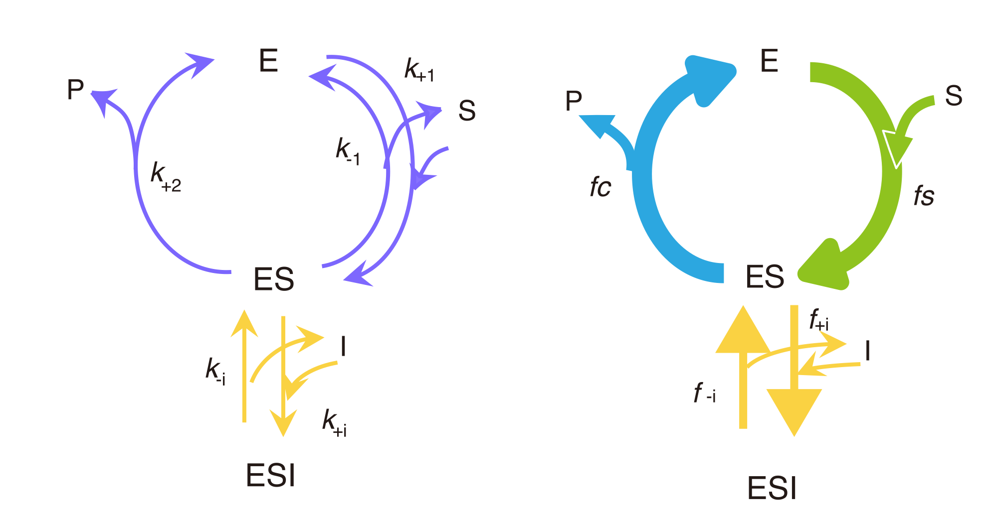
Figure 8. Uncompetitive Inhibition

Kinetic representation (left) and flux representation (right).

6. Acknowledgments

I thank Dr. Shinichi Miyairi, a former professor at the Nihon University School of Pharmacy, for numerous discussions and proofreading. Special thanks go to Professor Norio Niwa of the Nihon University School of Pharmacy for providing mathematical assistance in solving Equation (26). I also thank many students and Dr. Tomoko Takamiya, who collaborated with me in the research related to enzyme enhancers, which was the initial inspiration for this article.

Footnotes

¹It means the total flux is zero but the absolute value of flux _AB (→) is not. It means that the absolute value of flux _AB (→) is equal to the absolute value of flux _BA (←). Equilibrium is not synonymous with stagnation.

² Given the equation [E] + [ES] = [E] _total, Equation (2) implies that if ES is in a steady state, then E is also in a steady state.

³ Mathematically, Equations (3) and (5) are equivalent to the breakdown of Equation (2). However, Equation (3) and (4) explicitly show that both E and ES are in a steady state.

⁴ An outline of the derivation of the rate equation, Equation (9), is shown below.

(Equation (4))× k ₊₂ + (Equation (5))× k _-1 gives

  

$$(k_{-1}+k_{+2})f={k_{+1}k}_{+2}[E][S]$$(a)

Multiply by k ₊₁ k ₊₂[ S] to both sides of eq (a), then

$$k_{+1}{k}_{+2}[E][S]k_{+i}[I]=k_{+1}{k}_{+2}{k}_{-i}[\mathrm{\text{EI}}][S]$$

is rewritten as

  

$$\frac{k_{+i}}{k_{-i}}[I](k_{-1}+k_{+2})f={k_{+1}k}_{+2}[\mathrm{\text{EI}}][S]$$(b)

Multiply both sides of Equation (5) by $k_{+1}[S]$

  

$$k_{+1}[S]f=k_{+1}{k}_{+2}\left[\mathrm{\text{ES}}\right][S]$$(c)

Find a sum of Equations. (a), (b), and (c), then 　

  

$$[(k_{-1}+k_{+2})+\frac{k_{+i}}{k_{-i}}[I](k_{-1}+k_{+2})+k_{+1}[S]]f=k_{+1}{k}_{+2}{[E]}_{\mathrm{\text{total}}}[S]$$(d)

Equation (d) can be rewritten as Equation (9).

⁵ Equation (19) is familiar in most textbooks and is interpreted as that the apparent K _m value will increase by a factor of (1+[ I]/ K _i ), compared to the K _m value in the absence of the inhibitor. This equation can be rewritten as Equation ( e), where I and S have the same weight as the denominator. This expression may better explain the competitive nature of the substrate and inhibitor than Equation (19).

  

$$v\left(t\right)=\frac{V_{max}\frac{[S]}{K_m}}{1+\frac{[I]}{K_i}+\frac{[S]}{K_m}}$$(e)

6 Equation (19) cannot be applied if the inhibitor is a tight-binding inhibitor. In Equation (19), [ I] represents the concentration of the free inhibitor molecule. However, precisely speaking, [ I] = [ I] ₀ - [ EI], where [ I] ₀ is the nominal concentration of inhibitor I. When the binding affinity of the inhibitor is high ( e.g., K _i < 0.1nM), the inhibitor works at very low concentration: [ I] ₀ may be smaller or almost equivalent to the total enzyme concentration. In the case of such tight-binding inhibitors, [ I] could be much smaller than [ I] ₀, meaning that the approximation used in Equation (19), [ I] = [ I] ₀, is invalid.