Abstract
This study investigates the effects of latency in a real-time controlled networked robotic system by isolating the system into four main processes using high-speed camera and timestamp methods. The overall time delay was 1,057 to 2,479 ms, of which the time from when the network camera captures an image to when the host computer receives it accounted for 88.6 %. It was made clear that this time is the delay that should be given the most attention when building a remote monitoring and control system for small agricultural robots. It was also considered that this time delay would not be a fatal problem for tasks that do not require centimeter-order control, such as with weed mowing robots.
1. Introduction
Advances in autonomous small robot systems play an important role in various practical applications in smart agriculture and garden management. Small agricultural robots not only ensure safety and cost-effectiveness but also have high adaptability to electrification, which is consistent with the global goal of reducing carbon emissions (Saidani et al., 2021). Mowing robots are one of the most successful small field robots at present. One of the reasons for the success of many practical machines is that they operate under simple control by running inside a guide wire and eliminate expensive GNSS (global navigation satellite system) and IMU (inertial measurement unit). However, the fact that the work site relies on the burial of guide wires will be an obstacle to expanding to the management of multiple areas on a wide scale in the future (Ramnani et al., 2020).
Currently, state-of-the-art approaches often utilize GNSS and intelligent vision systems, which have demonstrated potential in addressing the challenges of autonomous agricultural robots. It can be seen that the development of an autonomous steering system for robotic mowers using GNSS and IMU has shown high accuracy in navigation over large terrains (Igarashi et al., 2022; Kaizu et al., 2018). Additionally, several studies have highlighted the feasibility of using machine vision to detect and remove weeds, as well as the potential for future integration with RTK (real time kinematic) GNSS and Lidar (laser imaging detection and ranging) systems (Quan et al., 2022; Visentin et al., 2023). Furthermore, trials using RGB-D cameras and IMU for position estimation and autonomous navigation of robotic mowers have proven effective even in areas with low GNSS accuracy (Inoue et al., 2022). However, these systems often rely on expensive sensors, are susceptible to environmental interference, and involve complex hardware-software configurations, which make maintenance and upgrades challenging (Xie et al., 2023). It can be noted that centimeter-level RTK-GNSS receivers and integrated GNSS and IMU packages suitable for precision agricultural tasks typically cost from a few hundred to several thousand US dollars, depending on performance class; this increases both hardware cost and system complexity. These limitations underscore the need for simpler yet efficient robotic systems, particularly for small-scale applications or areas with complex terrain.
The authors proposed an architecture that separates the intelligence function from the robot body and concentrates the computation function in a remote control station. A system based on this architecture was able to control and monitor the robot from a remote location via a network from a surveillance camera (Nguyen et al., 2024b). This system demonstrates a control method for a small robot that does not rely on guidewires or GNSS, but the time delay between receiving information from a surveillance camera and controlling the robot remains an issue.
It has long been argued that even a small delay in the time between sending a machine control command and the machine’s response can degrade system performance (Claypool et al., 2006; Green et al., 2021). Regarding latency over networks, Yu et al. (2022) investigated the impact of video streaming methods, such as TCP (transmission control protocol) and UDP (user datagram protocol) protocols, on the performance of remote driving. Their findings highlighted that stable and predictable latency are essential for effective control. Green et al. (2021) also measured the latency of wireless video transmission for remote agricultural machinery monitoring and highlighted that the transmission distance and video resolution significantly affect the delay. Similarly, Kaknjo et al. (2018) proposed a methodology to measure one-way video delays in a remotely operated vehicle system and revealed significant variations under various network conditions. Although previous studies examine the causes of delay and propose network-level optimizations, they generally omit a process-level, end-to-end analysis and the direct impact of these delays on real-time robotic control. Through this research, we will attempt to quantify the delay in controlling agricultural robots over a network, which is expected to contribute to safety in remotely monitoring robots.
In this study, we aim to develop a remote control and monitoring system for agricultural robots, with the goal of commercializing inexpensive field robots and promoting the general-purpose use of robot control infrastructure. This report focuses on clarifying the trends in latencies associated with communication, information processing, and control processes when remotely controlling a robot via a network camera. On the basis of the knowledge gained, we also consider control methods for a small robot that moves randomly in designated areas.
2. Materials and methods
2.1. Overview of test equipment and system architecture
The system presented in Fig. 1 consists of three main components: a network camera, a robot, and a host computer. A microcomputer (ESP32-CAM, Espressif Systems Co., Ltd., China) with a camera module (OV2640, Espressif Systems Co., Ltd.) was selected as the network camera due to its integration of both wireless connectivity and imaging capabilities. For the experiments, each video frame was independently compressed using the Joint photographic experts group (JPEG) encoding format, and consecutive JPEG images were streamed to form a motion JPEG (M-JPEG) video sequence.

Fig. 1
System overview
The crawler robot (HopeField Inc., Japan) (Fig. 2, Table 1) can move forward, backward, and rotate by controlling the rotational speeds of a pair of brushless DC motors (HK2445-KV3200, HobbyKing, China). The voltage supplied to these motors is regulated using two electronic speed controllers (ESCs) (QuicRUN-WP-16BL30, Hobbywing Technology Co., Ltd., China). In addition, a microcontroller equipped with a Wi-Fi communication module (ESP32, Espressif Systems Co., Ltd.) is used as the central component of the robot and provides wireless communication functionalities. The microcontroller on the robot as well as the network camera are programmed using the Arduino IDE (integrated development environment) (version 2.2.1., Arduino, 2023).

Fig. 2
Top view of crawler robot
Table 1
Hardware specifications of robot
| Traveling device |
Crawler |
| Size (L × W × H) |
(500 × 420 × 140) mm |
| Mass |
10.6 kg |
| Control method |
Skid steering (forward/reverse movement and steering by controlling rotation direction and speed of left and right crawlers) |
| Motor specifications |
Brushless DC motor (HK2445-KV3200, HobbyKing) |
| Driver |
Electronic speed controller (ESC) (QuicRUN-WP-16BL30, Hobbywing) |
| Power supply |
Main battery: 18 V DC, 6.0 Ah (108 Wh), Li-ion (BL1860B, Makita Corp. Japan)
Power converter output: 12 V DC, 3 A (36 W) for motors
|
| Central controller |
ESP32 (Espressif Systems Co., Ltd.) |
A remote computer monitors the robot’s operating area using a continuous stream of images transmitted from the network camera. A virtual boundary is created through a GUI (graphical user interface) developed using Python’s Tkinter library, in combination with OpenCV for real-time image stream processing. This virtual boundary enables the computer to supervise and control the robot’s random movements inside the defined area. The robot’s position is identified within the image frames, and control signals are transmitted to ensure the robot remains inside the specified boundary. All experiments were carried out on a single, stable Wi-Fi LAN (local area network) to provide a reproducible baseline for latency measurements. Representative measurements recorded on the host during testing showed RSSI (received signal strength indicator) values of −37 dBm and −29 dBm and observed transmission rates of approximately 130–144 Mbps.
While this study was conducted on a stable Wi-Fi LAN to ensure repeatable latency evaluation, other communication options could be considered for wider-range applications. Low-power wide-area (LPWA) technologies such as LoRaWAN can extend transmission distances to several kilometers but typically provide lower data rates (0.3–50 kbps), which may limit real-time image streaming (Augustin et al., 2016; Mekki et al., 2019). These trade-offs suggest that LoRaWAN or similar LPWANs may be more suitable for low-bandwidth sensing tasks rather than continuous video transmission. In contrast, cloud-based control platforms such as Blynk can simplify network integration and remote access, though additional delay from cloud routing would need to be evaluated in future work (Nguyen et al., 2024a).
2.2. Data processing and control logic
The system operation begins with the host computer sending a start request to the network camera to initiate the image acquisition and transmission process. Upon receiving the request, the network camera enters a loop in which it checks for available RAM (random access memory), captures an image if sufficient memory is available, and transmits the image to the computer. This loop continues until a termination request is received from the host computer. The received image frames are processed by the computer to detect the robot and determine its location.
In this study, the MOG2 algorithm (implemented as cv2.createBackgroundSubtractor-MOG2 in the OpenCV library) was applied to identify moving objects in the JPEG video stream received from the camera. MOG2 is a kind of background subtraction, and it is a widely adopted and computationally efficient technique for foreground segmentation in real-time applications (Matczak et al, 2021; Qasim et al., 2021; Zivkovic, 2004).
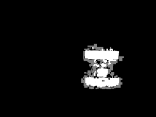
A background mask is generated after all input images (Fig. 3 (a)) are first converted to grayscale before processing. This mask is an image generated as the background where the robot travels using the 100 previous frames. We assume that the time-dependent fluctuation of each pixel is based on a Gaussian distribution, with pixels that deviate from the average being the foreground and the rest being the background. Next, the brightness of each pixel in the background mask and the processed image is compared. Those whose difference exceeds the variance threshold (set to 50 in this report) are recognized as moving objects (Fig. 3 (b)). Furthermore, among the pixels recognized as moving objects, any connected pixels are treated as a single cluster, and any masses less than 100 pixels in size are removed as noise. For each cluster, a cluster box (green rectangle in Fig. 3 (c)) that covers each cluster is determined. Finally, we define a detection box (red rectangle in Fig. 3 (c)) that covers all the cluster boxes determined, and its center point is set as the robot’s position.

(a)
Obtained image
(b)
Image after background masking
Fig. 3
Positioning of robot by MOG2 technique
Moving pixels were extracted in (b). Difference from mask image equals 50 in gray pixels. One is larger than 50 in white pixels. Yellow dot in (c) is center of detected box. Numbers in figure count cluster box.
Communication between the host computer and the robot is facilitated through the WebSocket protocol, which enables full-duplex communication over a single TCP connection. Both the computer and the robot’s microcontroller perform necessary WebSocket initialization during startup. Once the connection is established, the microcontroller ESP32 on the robot enters a continuous listening loop, awaiting incoming commands. If the robot is found outside the virtual boundary, the system issues a control command to the robot. Upon receiving a command, it acknowledges the task to the host, parses the instruction, and translates it into control signals that are sent to the motor drivers, resulting in wheel motion. This control loop persists until an explicit stop signal is received from the host computer.
2.3. Methods for measuring latency
2.3.1. Overview of latencies for remote control via LAN
The system architecture enables the division of communication flow into two primary closed-loop cycles: the first between the network camera and the host computer, and the second between the host computer and the robot. Owing to the closed-loop nature of each pairwise communication, the latency introduced in each cycle can be independently isolated and analyzed.
In the first communication cycle, which involves the network camera and the host computer, the measured latency is defined as the time elapsed from the moment an image is captured by the network camera to when it is displayed on the host computer’s monitoring screen. This cycle typically comprises several stages: image capture, data storage and processing at the network camera side, followed by data transmission, and finally, image receiving, processing, and visualization at the host computer.
To isolate and better understand the baseline latencies in this first communication round, we conducted two separate experiments. To evaluate the delay associated solely with image capture and transmission from the network camera to the computer, we configured the camera to continuously capture and send images, while the computer was tasked only with displaying each frame without performing any additional processing. This setup is defined as the image acquisition and transmission process (P1). In the second configuration, designed to clarify the time required for processing on the computer side, we measured the interval from when an image is received to when it is fully processed and rendered on the computer display. This is defined as the image processing process for robot detection (P2).
In the second communication cycle, which occurs between the host computer and the robot, the latency is defined as the time interval between the issuance of a control command by the host computer and the observable mechanical actuation of the robot’s crawler. To further isolate the sources of delay within this cycle, the process was decomposed into two functional sub-processes. Specifically, the control signal transmission process (P3) captures the time from when the host computer transmits a control signal to the moment the microcontroller on the robot successfully receives it via wireless communication. The full control-actuation process (P4), which encompasses P3, includes the time required for the microcontroller to decode the received command, execute the embedded control logic, and activate the motor driver circuitry to initiate crawler movement (Fig. 4).

Fig. 4
Data processing flow and time delay configuration
To ensure accurate evaluation of system latency, two complementary measurement methods were used: a HSC (high-speed camera) for high-precision visual observation, and a timestamp-based approach using the computer’s internal clock. The timestamp method leverages the computer’s internal clock to record the start and end times of each process. By comparing timestamps from different processes, the delays introduced by individual components of the system can be quantified (Green et al., 2021; Kaknjo et al., 2018).
However, the timestamp method is not applicable for measuring latency in processes that involve physical movements, such as P4, where the microcontroller initiates control of the power circuits, and the wheels of the robot begin to move. This is because the timestamp method cannot capture external motion, which can only be accurately measured through observable physical changes. Additionally, incorporating an extra process to display and record timestamps during control operations introduces minor delays. Although these delays are generally negligible and do not significantly affect the system, they must be considered when analyzing results.
Due to these limitations, HSC was used to evaluate latency in scenarios where timestamping was inadequate. The HSC method provides an independent and precise measurement by visually capturing system outputs at high frame rates. Ideally, the latency across all processes, from image transmission to robot control, would be evaluated solely using the HSC. However, practical constraints make this approach challenging. As a result, the system was divided into distinct processes, and each process was evaluated independently using a HSC (HAS-U1M, DITECT Co. Ltd., Japan.) where applicable. Images were captured at 1,000 frames per second (fps) at QVGA resolution. Recording and analysis were processed using control software (HAS-XV Viewer version 1.3.10.2, DITECT Co. Ltd.) that allowed frame-by-frame examination of time-critical events. The host computer, running macOS Ventura 13.3, operated a Python-based software platform developed specifically for this experiment. All control logic, image acquisition routines, and timestamp logging processes were implemented in Python 3.12.4 using VSC (visual studio code) (version 1.90.2). The software was designed to: (1) send periodic capture requests to the network camera, (2) receive and decode M-JPEG streams, (3) process image frames using OpenCV (e.g., MOG2 for foreground extraction and contour detection), (4) compute positional boundaries, and (5) send control commands to the microcontroller on the robot via the WebSocket protocol. Timestamp logging for each subprocess was integrated to allow precise latency calculation. All log data were saved to CSV files for subsequent analysis.
2.4. Experimental setup for latency measurement
2.4.1. Measurement of image acquisition and transmission process (P1)
The time for the image acquisition and transmission process (P1) was measured using the HSC system. To measure P1, images of a digital clock, which displayed in 1/100 s increments, were transmitted to a host computer via the network camera, and the digital clock and the host computer monitor were photographed with a HSC (Fig. 5). The frame rate of the network camera in this setup was 50 fps at a VGA resolution of (640 × 480) pixels. The host computer then displayed the received images in real time. The host computer used in these experiments had a display refresh rate of 60 Hz. Identifying output changes on the basis of HSC image data may introduce errors due to this refresh rate, calculated as follows: 1/60 = 16.667 ms. However, since screen latency is also part of the system under study, this error margin is not reduced in this research. Finally, the HSC was positioned to simultaneously record both the time on the digital clock and on the computer display.

Fig. 5
Set-up testing latency measurement in image acquisition and transmission process
Latency for P1 was measured by capturing video footage using the HSC that simultaneously recorded both the digital clock and the host computer’s screen. The network camera continuously captured the digital clock and transmitted the images to the host computer. The host computer then displayed the received images on its screen. To determine latency, two key frames were identified in the HSC footage: the first showing the updated time value on the physical digital clock, and the second showing the same time value on the computer screen. The difference in frame indices between these two events represents the end-to-end latency for the image acquisition and transmission process.
Next, the timestamp method was also used. When the network camera begins capturing an image, it transmits a signal to the host computer. This signal is logged using the Serial Monitor of the Arduino IDE (installed on the host computer) and includes both the image index and the timestamp indicating when the capture command was initiated. This data is transmitted via a standard micro USB wired connection. The captured image is subsequently sent to the computer over a LAN network. When the computer receives and displays the image in VSC, a corresponding timestamp is recorded. Latency is calculated as the difference between the two recorded timestamps.
2.4.2. Measurement of image processing process on host computer (P2)
To measure the latency of the image processing process on the host computer (P2), an experiment using the HSC method was conducted, where the robot continuously rotated in a fixed direction within the surveillance area of the network camera, which transmitted image frames in real time to the host computer. Upon receiving each frame, the VSC monitoring application displayed an indicator confirming image receipt. Once the processing was completed—including object detection, contour extraction, and virtual boundary—the final processed image was rendered on the screen.
Two critical events were identified in the recorded footage. Event (1): The appearance of printed text on the terminal screen in VSC, indicating that the computer has received a new image frame. Event (2): The moment when the corresponding processed image appears on the computer screen after the object detection and processing phase is complete. Latency was computed by counting the number of frames between these two events in the HSC footage.
2.4.3. Measurement of control command transmission process (P3)
The user interface implemented in VSC displays five control buttons (i.e., Go Forward, Stop, Go Backward, Turn Left, Turn Right) on the screen of the host computer (Fig. 6) in order to evaluate the latency of the control command transmission process. Every time the operator clicks each button, the robot, which is equipped with a microcontroller with a Wi-Fi module, receives the corresponding control commands via the wireless LAN. To facilitate precise latency measurement during this process, a standard micro USB cable was used to establish a direct connection between the microcontroller on the robot and the host computer. This setup enabled real-time serial communication, allowing the microcontroller to print the exact timestamp to the Arduino IDE’s serial monitor at the moment it received the control command. Two specific time points were recorded at the host computer to calculate latency: the moment when a control button was pressed and released on the host computer’s screen, and the moment when the robot received the command via LAN and responded by printing the timestamp to the Serial Monitor. The difference between these two timestamps represents the latency of the control command transmission process (P3).

Fig. 6
Set-up testing latency measurement in sending and receiving command and robot’s response
A user interface with five control buttons is displayed on the screen of the host computer (Fig. 6), similar to the setup used in the measurement of the control command transmission process. The HSC then records the moment any control button is pressed and released. The system sends a control signal to the robot, and the HSC records the subsequent wheel movement of the robot. By reviewing the HSC footage, the number of frames between the button release and the movement of the robot’s wheels can be counted. In this process, there are two important moments that need to be considered: the moment a control button is released and the moment the wheels start moving. The difference between these two times, alongside the corresponding images, defines the latency for this process.
3. Results
3.1. Latency measurement results for image acquisition and transmission process (P1)
Figure 7 presents the latency distribution for the image acquisition and transmission process (P1), as measured using both the HSC and timestamp-based methods. The majority of latency values obtained via the HSC method were tightly concentrated around 1,250 ms, with more than 70 % of the data falling into this single class. In contrast, the timestamp method exhibited a broader and more varied distribution, with values spread widely across the range from 250 to over 2,250 ms.
Despite this difference in distribution, the mean latency values were similar: 1,335 ms for the HSC method and 1,363 ms for the timestamp method. However, the timestamp results demonstrated greater dispersion and a higher frequency of extreme latency values. This contrast is visually apparent in the histogram, where the HSC data shows a sharp peak, while the timestamp data is more widely distributed. These results provide a direct visual and statistical comparison between the two methods for this process.
To verify the statistical characteristics of latency distributions, a Shapiro–Wilk normality test was conducted for both measurement methods (HSC and timestamp). For the latency distribution measured by HSC, the test statistic (W) was 0.231, and the p-value (p) was less than 0.01. For another distribution, measured using the timestamp method, W was 0.833, and p was also below 0.01. Therefore, both distributions deviated from normality, mainly due to the presence of occasional high-delay outliers. In addition, the median latency values were 1,157 ms for the HSC method and 1,177 ms for the timestamp method, both close to their respective means. This indicates a consistent central tendency between the two measurement approaches, despite differences in distribution shape.
3.2. Latency measurement results for image processing process (P2)
Figure 8 illustrates the latency distribution for the image processing process (P2), measured using the HSC method. Most of the latency values were concentrated between 8 to 12 ms, accounting for approximately 73.3 % of the total measurements. The mean latency was 14.38 ms, with a standard error of 0.55 ms, indicating relatively consistent performance with moderate variability.
Notably, the distribution displayed a bimodal pattern: a dense cluster of values from 8 to 14 ms, followed by a gap, and then a second group between 24 to 30 ms. This discontinuity may be attributed to frame quantization effects or synchronization delays during high-speed recording, which can occasionally introduce jumps in latency measurements. Despite this, the main concentration of values supports the reliability of the processing time estimates.
3.3. Latency measurement results for control signal transmission process (P3)
The latency measurements for process P3 using the timestamp method are shown in Fig. 9. The results indicate that the majority of latency values fall within the range of 50 to 175 ms, comprising approximately 88.6 % of all recorded measurements. The mean latency for this process was 120.63 ms, with a standard error of 1.19 ms.
The latency distribution for P3 exhibits a right-skewed pattern, with most values concentrated around 100–150 ms and a long tail extending toward higher latencies. This indicates that while the control signal transmission process is generally stable, occasional spikes in delay occur, likely due to transient network congestion or concurrent data transfer with the image stream. Such sporadic latency increases could momentarily degrade the responsiveness of robot control, particularly during rapid maneuvering or near obstacles.
3.4. Latency measurement result for full control-actuation process (P4)
Process P4 represents the stages where the computer sends control signals to the robot. The total latency in this process includes several components: the delay in displaying commands on the computer screen, network transmission latency, signal decoding time, and the delay associated with power transmission to the robot’s crawler. The measurement results for this total process are illustrated in Fig. 10. Latency values are primarily concentrated in the range of 75 to 200 ms, with the highest recorded delay reaching 646 ms. The mean latency for this process was 156.8 ms, with a standard error of 6.94 ms.
4. Discussion
4.1. Evaluation and usage of timestamp information
The time for the image acquisition and transmission process (P1) was measured using two methods: HSC and timestamp. As shown in the method section, the evaluation target and the evaluation device should be separated, and the management of the timestamp itself also affects the control system, so it can be understood that the results of the timestamp are only for reference. As shown in Table 2, the mean latency for P1 was 1,335 ms using the HSC method and 1,363 ms using the timestamp method. Despite the slightly higher average in the timestamp data, both methods showed comparable central tendencies (median values of 1,157 ms for HSC and 1,177 ms for timestamp), suggesting a generally close alignment. However, the distributions differed significantly. The timestamp-based measurements exhibited a much broader distribution (range = 10,161 ms, standard deviation (SD) = 1,096 ms), with values spanning from as low as 2.3 to over 10,000 ms. In contrast, the HSC data were more concentrated (range = 9,914 ms, SD = 948 ms), and a histogram revealed a more symmetrical profile centered around 1,000 to 1,300 ms. For the time of the control signal transmission process (P3), measurements could not be taken with a high-speed camera, so measurements were taken only using the timestamp. Considering the comparison of HSC and timestamp for P1, the reliability of representative values such as the average and median for the results of P3 is high. The time of the full control-actuation process (P4) is the time from sending the command to the robot’s operation, of which the time required for communication is P3, and the difference between P4 and P3 can be separated as the time from receiving the command to the robot’s operation.
Table 2
Measurement results for each process and method
| Measurement process |
Measurement method |
Number of data |
Median (ms) |
Mean (ms) |
Standard deviation |
| P1: image acquisition
|
HSC |
173 |
1,157 |
1,335 |
948 |
| Time stamp |
2,619 |
1,177 |
1,363 |
1,096 |
| P2: image processing
|
HSC |
180 |
11 |
14.38 |
7.37 |
| P3: control signal transmission
|
Time stamp |
2,380 |
113 |
120.63 |
58.26 |
| P4: full control-actuation
|
HSC |
107 |
149 |
156.8 |
71.83 |
While the HSC and timestamp methods together provide complementary views on system latency, each method has inherent limitations that affect interpretation. HSC offers direct, frame-level observation of external outputs (screen updates, motor motion) and serves as a practical ground truth for visible events. However, it is not a field-deployable instrument for routine monitoring (setup cost and complexity), and its measurements are subject to frame-quantization, camera viewpoint, lighting conditions, and interaction with the host display’s refresh rate. Conversely, timestamp logging on the host is inexpensive and scalable for large datasets, but timestamps reflect events inside the system and can be affected by logging overhead, non-deterministic background tasks, and clock synchronization issues; thus, timestamps may under- or over-estimate short, internal delays. Importantly, our experiments were performed on a single configuration, so the reported values are context-specific and should be interpreted as a practical reference for similar commodity M-JPEG-over-Wi-Fi deployments.
4.2. Overview of total latency and its reflection to control
Although there are some overlaps in processing and some parts that are difficult to estimate, the time from acquiring the image to controlling the robot is generally calculated as the sum of P1, P2, and P4. The average value of the measurement results using HSC for each item is summed up to 1,507 ms, and considering the variability of the data, it is generally within the range of 1,057 to 2,479 ms. Of this, the time to acquire images via the LAN (P1) accounts for 88.6 % of the total. Control commands from the host computer to the robot are also sent via the LAN, but the time of P3 is extremely short compared to P1. This is thought to be due to the difference in the size of the data exchanged since P1 receives images. From the above, the most important process in discussing delays in real-time monitoring and control is the processing from acquiring images with a network camera to receiving them with a host computer.
If the time required for P1, P2, and P4 is 1,057 to 2,479 ms and the robot’s movement speed is 0.2 m/s (Chosa et al., 2024), the robot will move about 0.21 to 0.5 m while communicating and processing images. For tasks that do not require centimeter-order control, such as a weed mowing robot, this time delay does not have a serious impact. However, the tested configuration is not suitable for applications requiring centimeter-level accuracy (e.g., precision planting or intra-row weeding) because the observed delays would produce position errors far exceeding such tolerances unless additional compensation is implemented. Although not verified in this study, position recognition errors may have greater impact than time delays. In addition, in tasks using a weed mowing robot that do not require high-precision control, it is important to stay within the specified range and to avoid collisions with obstacles, including people. Therefore, measures that can be considered include taking into account time delays and performing control to avoid obstacles early, or predicting the robot’s position at the time of control and determining control commands. Another effective measure would be to slow down the robot’s speed in the vicinity of boundaries and obstacles to prevent it from going beyond those boundaries. Since it takes time to transmit images, a possible solution would be to reduce the amount of data transmitted and received by introducing preprocessing. Such control and data transmission measures that take into account time delays need to be verified through simulations and actual work.
For practical field deployment, we provide a simple, directly usable rule of thumb based on the measured end-to-end delay for P1, P2, and P4. Using the mean HSC-based total delay of approximately 1,507 ms, a useful design guideline is: expect the vehicle to travel roughly 0.15 m per 0.1 m/s of forward speed while the system processes and reacts. In operational terms, this means a mower moving at 0.2 m/s may become displaced about 0.30 m; at 0.5 m/s, the corresponding displacement approaches 0.75 m. For conservative design, we recommend applying a safety buffer equal to this expected displacement when specifying boundary offsets, obstacle-clearance margins, or speed-reduction thresholds. In practice, adopting such buffers, combined with slowed operation near boundaries and local proximity sensing for emergency stops, provides a straightforward means of maintaining safety when using similar low-cost M-JPEG over Wi-Fi systems.
4.3. Impact of latency on remote monitoring via network camera
The experimental results reveal that the most significant time delay occurs in the image acquisition and transmission process (P1), with an average latency of approximately 1,335 ms. In a fully automated system where a host computer performs object detection and boundary checking based on incoming video frames, such a delay introduces a substantial risk: the analysis and subsequent decisions are always made on the basis of outdated visual information.
This outdated perception can lead to inaccurate assessments of the robot’s position relative to the virtual boundaries. As a result, the host computer may issue control commands too late to prevent undesired behavior, such as the robot crossing a boundary or missing a target area. Therefore, the latencies that arise during data acquisition and robot control in general need to be addressed. To mitigate this issue, compensating for known delays through predictive control strategies or latency-aware boundary estimation should be considered in future studies.
Recent studies demonstrate concrete, directly applicable delay-compensation strategies that motivate our next steps. (Das et al., 2021) propose an augmented-state extended Kalman filter (AS-EKF) that explicitly models uncertain, time-varying measurement delays and thereby estimates the robot’s current pose from delayed sensor data. Complementing state-estimation methods, (Chakraborty et al., 2025) present a learning-based pipeline for generating delay-compensated video frames for outdoor teleoperation; their approach predicts or synthesizes up-to-date visual frames from delayed streams and was validated on real outdoor robot data. Based on these works, two concrete follow-up directions are proposed: (1) implement a delay-aware state estimator to predict the robot’s true pose, and (2) investigate frame-level compensation (learning- or model-based) so that the perception pipeline processes latency-compensated images. We will experimentally evaluate these approaches to determine whether compensation can mitigate the latency observed in our setup.
5. Conclusions
This study focused on a remote monitoring and control system for agricultural robots. The process from image acquisition to real-time robot control was divided into four processes: 1) from acquiring images using a network camera to receiving them at the host computer via wireless LAN, 2) from the received images to the host computer recognizing the robot’s position, 3) sending control commands from the host computer and receiving the control commands at the robot via wireless LAN, and 4) from receiving the control commands to the robot’s operation. The time delays in each process were analyzed.
Although precise separation of these processes was not possible and some processing was estimated from timestamp information managed by the host computer, the overall processing time was between 1,057 and 2,479 ms. In addition, more than 88.6 % of this was the time from acquiring images using a network camera to receiving the images at the host computer via wireless LAN. These numerical values quantify system behavior for the specific low-cost hardware, software, and Wi-Fi conditions used in our experiments; they are therefore context specific rather than universal bounds. Nevertheless, they provide a practical reference for similar commodity, M-JPEG-over-Wi-Fi deployments and show that including host computer processing and actuation can substantially increase total latency relative to video-only measurements.
Table 3 summarizes representative latency values reported in prior studies alongside our results. Prior work has focused mainly on single components of the sensing-control chain: Yu et al. (2022) report sub-50 ms latency for an optimized UDP streaming pipeline in a laboratory Wi-Fi setup, Kaknjo et al. (2018) measured video latencies of around 488–850 ms on LAN and about 558–1,211 ms over the Internet for off-the-shelf IP cameras, and Green et al. (2021) report lower-hundreds-of-milliseconds delays in wireless video links for agricultural supervision. In contrast, our measurements quantify the full operational path relevant to closed-loop supervision. Because prior studies typically report video-only or component-level delays under different hardware and transport configurations, direct numeric comparisons are indicative rather than exact; nevertheless, the comparison clarifies that when host processing and actuation are included, low-power, commodity hardware and standard M-JPEG over Wi-Fi can yield substantially larger total latencies than video-only, optimized streaming scenarios. This process-level, end-to-end characterization—validated by high-speed camera—is the primary contribution of the present work.
Table 3
Comparison of observed total path latency with earlier studies
| Study |
System/test conditions |
Reported latency |
| Green et al., 2021
|
Real-time wireless video for remote supervision of agricultural machines; cellular and radio links tested. |
Under about 300 ms |
| Yu et al., 2022
|
Designed remote driving system; compared streaming schemes (UDP-based low-latency streaming). Reported targeted/achieved low-latency UDP streaming (optimized). |
Achieved lower than 50-ms latency |
| Kaknjo et al., 2018
|
Measured video latencies using NTP sync and instrumentation (LAN vs Internet) for an off-the-shelf IP camera. |
Reported LAN: 488–850 ms;
Over Internet: 558–1,211 ms
|
| This study |
Network camera (ESP32-CAM) to host computer processing to ESP32 robot; per-process breakdown P1–P4.
|
Observed total path (P1+P2+P4) around 1,057–2,479 ms.
|
The time delay from acquiring the image to controlling the robot is approximately 1,057 to 2,479 ms, and if the robot’s movement speed is 0.2 m/s, then this results in an error of 0.21 to 0.5 m. For tasks that do not require centimeter-order control, such as using a grass-cutting robot, it is believed that the effects of time delay will not be a fatal problem. Alternatively, it may be possible to reduce the effects of time delay by devising a control method that takes this effect into account, or by using pre-processing methods to reduce the size of the data to be transferred. These hypotheses need to be further examined through verification via simulations and actual work.
In summary, the novelty of this research lies in its quantification of latency and clarification of its variability across each process (P1–P4) within a single network camera-based robotic control system. Although the results are limited to the specific low-cost hardware, software, and Wi-Fi conditions used in our experiments, they are expected to serve as a minimum benchmark for system design in the future development of remote monitoring technology, especially as CPU processing speeds and communication environments continue to improve.
Acknowledgments
This work was supported by JSPS KAKENHI Grant Numbers 23K27030.
Declaration of conflicting interests
The authors declare no conflicts of interest.
Notes
(URLs on references were accessed on 6 February 2026.)
References
- Arduino. 2023. Arduino IDE. Version 2.2.1. Italy: Arduino Foundation. https://github.com/arduino/arduino-ide/releases
- Augustin, A. et al. 2016. A study of LoRa: Long range & low power networks for the internet of things. Sensors. 16 (9): 1466. https://doi.org/10.3390/s16091466
- Chakraborty, N. et al. 2025. Towards real-time generation of delay-compensated video feeds for outdoor mobile robot teleoperation. Proceedings of the 2025 IEEE International Conference on Robotics and Automation (ICRA). 1097–1104. https://doi.org/10.1109/ICRA55743.2025.11128424
- Chosa, T. et al. 2024. Motion analysis of a robot that performs tasks by running randomly. Proceedings of the 11th International Symposium on Machinery and Mechatronics for Agriculture and Biosystems Engineering (ISMAB). GT-R1.
- Claypool, M. et al. 2006. Latency and player actions in online games. Communications of the ACM. 49 (11): 40–45. https://doi.org/10.1145/1167838.1167860
- Das, B. et al. 2021. Delay compensated state estimation for Telepresence robot navigation. Robotics and Autonomous Systems. 146: 103890. https://doi.org/10.1016/j.robot.2021.103890
- Green, M. et al. 2021. Measurement of latency during real-time wireless video transmission for remote supervision of autonomous agricultural machines. Computers and Electronics in Agriculture. 190: 106475. https://doi.org/10.1016/j.compag.2021.106475
- Igarashi, S. et al. 2022. Autonomous driving control of a robotic mower on slopes using a low-cost two-frequency GNSS compass and an IMU. Journal of the ASABE. 65 (6): 1179–1189. https://doi.org/10.13031/ja.15032
- Inoue, K. et al. 2022. Autonomous navigation and obstacle avoidance in an orchard using machine vision techniques for a robotic mower. Engineering in Agriculture, Environment and Food. 15 (4): 87–99. https://doi.org/10.37221/eaef.15.4_87
- Kaizu, Y. et al. 2018. Development of an autonomous driving control system for a robot mower using a low-cost single-frequency GNSS and a low-cost IMU. Journal of the Japanese Society of Agricultural Machinery and Food Engineer. 80 (5): 271–279. (In Japanese.) https://doi.org/10.11357/jsamfe.80.5_271
- Kaknjo, A. et al. 2018. Real-time video latency measurement between a robot and its remote control station: Causes and mitigation. Wireless Communications and Mobile Computing. 2018: 8638019. https://doi.org/10.1155/2018/8638019
- Matczak, G. et al. 2021. Comparative Monte Carlo analysis of background estimation algorithms for unmanned aerial vehicle detection. Remote Sensing. 13 (5): 870. https://doi.org/10.3390/rs13050870
- Mekki, K. et al. 2019. A comparative study of LPWAN technologies for large-scale IoT deployment. ICT express. 5 (1): 1–7. https://doi.org/10.1016/j.icte.2017.12.005
- Nguyen, V. D. et al. 2024a. A cost-effective and simplified approach of the remote control system for agricultural small robots. Proceedings of the 59th Annual Meeting of KANTO Society of Agricultural Machinery and Food Engineers. 23–24.
- Nguyen, V. D. et al. 2024b. Development of the small robot management system using a network camera. Proceedings of the 11th International Symposium on Machinery and Mechatronics for Agriculture and Biosystems Engineering (ISMAB). BR-R18.
- Qasim, S. et al. 2021. Performance evaluation of background subtraction techniques for video frames. Proceedings of the 2021 International Conference on Artificial Intelligence (ICAI). 102–107. https://doi.org/10.1109/ICAI52203.2021.9445253
- Quan, L. et al. 2022. Intelligent intra-row robotic weeding system combining deep learning technology with a targeted weeding mode. Biosystems Engineering. 216: 13–31. https://doi.org/10.1016/j.biosystemseng.2022.01.019
- Ramnani, S. M. et al. 2020. Unmanned automated lawn mower. International Research Journal of Engineering and Technology. 7 (6): 2473–2484.
- Saidani, M. et al. 2021. Comparative life cycle assessment and costing of an autonomous lawn mowing system with human-operated alternatives: Implication for sustainable design improvements. International Journal of Sustainable Engineering. 14 (4): 704–724. https://doi.org/10.1080/19397038.2021.1919785
- Visentin, F. et al. 2023. A mixed-autonomous robotic platform for intra-row and inter-row weed removal for precision agriculture. Computers and Electronics in Agriculture. 214: 108270. https://doi.org/10.1016/j.compag.2023.108270
- Xie, B. et al. 2023. Research progress of autonomous navigation technology for multi-agricultural scenes. Computers and Electronics in Agriculture. 211: 107963. https://doi.org/10.1016/j.compag.2023.107963
- Yu, Y. et al. 2022. Remote driving control with real-time video streaming over wireless networks: Design and evaluation. IEEE Access. 10: 64920–64932. https://doi.org/10.1109/ACCESS.2022.3183758
- Zivkovic, Z. 2004. Improved adaptive Gaussian mixture model for background subtraction. Proceedings of the 17th International Conference on Pattern Recognition (ICPR 2004). 2: 28–31. https://doi.org/10.1109/ICPR.2004.1333992


