Real-time risk assessment framework for tractors: part 2
— Risk point estimation using discriminant analysis based on behaviour —

2026 Volume 19 Issue 3 Pages 153-161
Details
2026 Volume 19 Issue 3 Pages 153-161
We present a behaviour-based, real-time estimator of tractor rollover risk suitable for embedded use. A four-degree-of-freedom vehicle model generated labelled scenarios across speeds (0.5–4.0 m/s), slope angles (0–20 °), and ISO 8608 roughness classes. Two closed-form discriminants for pitch and roll require only three onboard signals—vehicle speed, vertical acceleration, and a 0.3 s double-integrated angular-acceleration angle. On simulated runs, the pitch discriminant achieved 96.4 % sensitivity and specificity; the roll discriminant reached 100 % and 99.5 %, with mean lead times of 0.88 s and 0.53 s before rollover onset. Discriminant scores are mapped to a unified Risk Point scale, enabling interpretable warnings for proactive operator assistance during field and road operation.
Accidents involving agricultural tractors represent a major occupational hazard worldwide and account for a significant proportion of agricultural incidents (Gilblom et al., 2023; Khadatkar et al., 2022; MAFF, 2023). Rollovers constitute a particularly large proportion of these accidents (Arana et al., 2010; MAFF, 2023). In addition to physical injuries to operators, these accidents lead to considerable economic losses due to structural damage to the tractor itself.
One of the primary reasons for the high frequency of rollover accidents is the distinctive structural design of tractors compared with that of passenger vehicles. For example, tractors are typically not equipped with wheel suspensions; therefore, vibrations and shocks caused by ground unevenness are directly transmitted to the entire chassis, meaning that the tires serve as the main means of shock absorption. Furthermore, their large tires and high ground clearance raise the centre of gravity, making tractors inherently unstable. Tractor designs commonly feature rear wheels that are larger than the front wheels, which, together with the installation of rollover protective structures (ROPS) and implements, shift the centre of gravity further rearward. Previous studies have shown that these special structural characteristics cause tractors to exhibit nonlinear dynamic behaviour unique to this type of machine (Garciano et al., 2005; Sakai et al., 1999). This nonlinear behaviour includes amplitude-dependent responses and abrupt growth of vibrations that can rapidly erode stability margins. Depending on the surface profile and driving speed, tractors can undergo resonance phenomena in which the tractor bounces violently, leading to dangerous vibrations (Garciano et al., 2002; Sakai et al., 2000). When such nonlinear dynamics occur during field operations, instability can escalate within a very short period, leaving insufficient opportunity for operators to take corrective actions, resulting in accidents (Watanabe et al., 2019).
Rollover warning devices have been developed as safety measures for tractors. Most conventional systems rely on threshold values of the tilt angle; once the threshold is exceeded, an alarm is triggered to prompt evasive action by the operator. However, in cases of rollover due to nonlinear dynamics, the vehicle may surpass the threshold angle almost instantaneously, leaving insufficient time for a response after the alarm. Moreover, these systems do not activate when the tilt angle is below the threshold but approaching it, and thus cannot continuously assess ‘how close’ the tractor is to the rollover boundary. To prevent accidents proactively, operators must be prompted to take action before reaching the threshold. Therefore, a framework that can detect rising risks in advance and alert the operator before a rollover occurs is required.
In Part 1 of this study, we introduced the concept of risk points (RPs) based on accident factors and proposed a framework for visually presenting potential risks in the working environment. Potential risks exist around tractor working situation are composed by factors changing slowly likewise temperature and brightness or so. Framework for estimates such risk level is essential because it is difficult for operators to know it. On the other hand, estimation for manifest risk is also important. Tractor related accidents have cases of rollover caused by wheels dropping off, running over steep incline or loss of vehicle attitude on slope and which end up operators to serious injury. Accordingly, this paper (Part 2) (1) proposes a rollover prediction model that leverages the dynamic state variables of the tractor, and (2) translates instability levels into ‘RPs based on tractor behaviour’, (3) By aligning these behaviour-based RPs with the RP scale introduced in Part 1, static risk awareness and dynamic risk evaluation are integrated into a unified scale.
The developed classification model predicts rollovers and evaluates RPs based on tractor behaviour data. The estimation process consists of two phases: rollover prediction and RP conversion (Fig. 1).

In the rollover prediction phase, the model determines the likelihood of a rollover using a prediction equation, denoted as τ (v, p, az) for a pitching rollover and τ (v, r, az) for a rolling rollover. A pitching rollover occurs when the tractor tips forward or backward due to steep slopes or obstacles, whereas a rolling rollover occurs when the tractor tips sideways due to lateral slopes or centrifugal forces. If the output of this equation is greater than or equal to the threshold C, a rollover is predicted; if it is less than C, no rollover is predicted.
In the subsequent RP conversion phase, the model calculates a behaviour-based RP using a conversion equation denoted as Ι. The parameter γ represents the degree of proximity between the prediction output τ and the threshold C, and it is used to quantify how close the tractor’s dynamic state is to a rollover condition.
2.1. Rollover prediction equationThe rollover prediction equation was formulated through discriminant analysis of behavioural data obtained from tractor driving and rollover simulations.
2.1.1. Simulation conditions 2.1.1.1. Travelling velocityTravelling velocities ranging from 0.5 m/s to 4.0 m/s were adopted in 0.5 m/s increments. A velocity of 0.5 m/s was chosen to represent low-speed field operations, whereas 4.0 m/s reflects typical road travel conditions.
2.1.1.2. Road surface inclination and roughnessTwo types of road surface inclinations were modelled: longitudinal inclinations to simulate pitching rollovers and lateral inclinations to simulate rolling rollovers. The inclination angles ranged from 0 ° (flat terrain) to 20 ° (reflecting typical slopes found in hilly farmland and orchards).
Road surface roughness was generated using the inverse Fourier transform, based on the relationship between the roughness levels (defined by ISO 8608 [ISO 8608:2016, 2016]) and the power spectral density of the road shape frequency. The roughness levels were classified as follows.
Very Good: equivalent to smooth concrete pavement
Good: smooth paved road
Normal: smooth unpaved road
Poor: rough unpaved or gravel road
Very Poor: uneven terrain or rough grassland
The total length of the terrain data was 540 m. Of this, 40 m was allocated to stabilise the transient vibration caused by the initial conditions, followed by 100 m of simulated road distance for each roughness level. An example of a terrain surface with no incline is shown in Fig. 2.
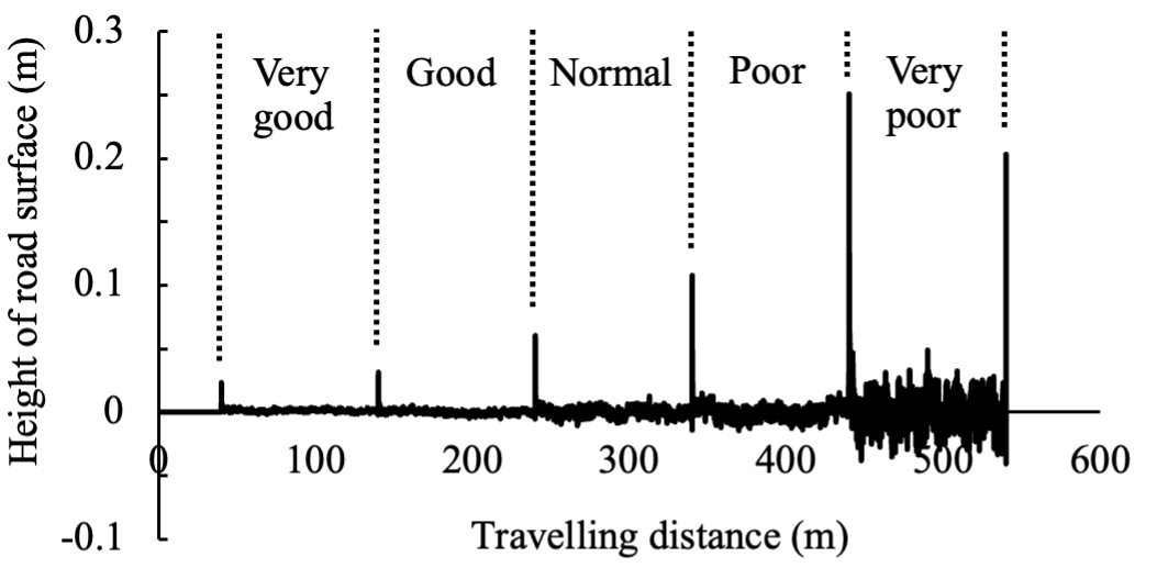
A four-degree-of-freedom (4-DOF) tractor motion model, developed by Matsui et al. (2017), was used in this study. The model was implemented in MATLAB/Simulink and mechanically represents motion with four degrees of freedom: longitudinal (forward/backward), vertical (up/down), pitch rotation, and roll rotation. It also incorporates the pivot mechanism of the front axle, which is a standard feature of typical agricultural tractors.
The specifications of the tractor used in the simulation are summarised in Table 1.
| Specification item | Value |
|---|---|
| Body mass (kg) | 1,010 |
| Wheelbase (m) | 1.5 |
| Tread (m) | 1.05 |
| Distance between mass center and ground (m) | 0.91 |
| Distance between mass center and rear axle (m) | 0.75 |
| Front wheel spring coefficient (N/m) | 60,000 |
| Front wheel damping coefficient (N s/m) | 200 |
| Rear wheel spring coefficient (N/m) | 160,000 |
| Rear wheel damping coefficient (N s/m) | 4,400 |
| Inertia moment of pitching (kg m2) | 600 |
The key contributors to tractor rollover are travelling velocity, road surface roughness, and vehicle orientation. Therefore, the following three variables were selected as predictors in the rollover discriminant analysis: travelling velocity (m/s), vertical acceleration (m/s2), and the evaluated angle (rad).
The evaluated angle was calculated as follows.
| (1) |
| (2) |
Here, p and r represent the angles evaluated for pitch and roll, respectively. Each is calculated by adding the result of a double time integration of angular acceleration (
Although the body inclination angle reflects the tilt of the tractor at a specific moment, it does not capture the trend or trajectory of the tractor’s motion. In contrast, the angular acceleration indicates whether the tractor’s motion is progressing toward or away from the critical rollover angle. By applying double integration, the dimensionality is aligned with the angular position, and the result can be interpreted as a predictive indicator of rollover behaviour. The integration interval used for this calculation was set to 0.3 s.
2.1.4. Method of discriminant analysisBehavioural data obtained from the simulations—sampled at 0.01-second intervals—were labelled as 0 or 1, depending on whether the data were gathered before or after the tractor reached its static rollover angle. For the studied tractor model, the static pitching rollover angle was 0.36 rad and the static rolling rollover angle was 0.52 rad.
Discriminant analysis was conducted separately for the datasets corresponding to the longitudinal and lateral inclinations of the road. Parameter optimisation was performed using 4-fold cross-validation implemented using MATLAB’s Statistics and Machine Learning Toolbox. The threshold for the resulting discriminant function was determined based on the intersection point of the sensitivity–specificity curve, which represents the optimal balance between sensitivity and specificity.
2.2. Risk point conversion equation ΙThe rollover prediction equation determines whether a rollover is likely to occur by comparing the equation output value τ with a predefined threshold C. The proximity of τ to this threshold can indicate behavioural risk. To reflect this, a conversion from behavioural data to an RP was defined based on the degree of alignment between the prediction output τ and the threshold C.
As illustrated in Fig. 1, the matching rate γ (%) is calculated using Eq. (3).
| (3) |
When τ exceeds the threshold C, τ reaches 100 % or higher, indicating that the tractor is in a rollover state. However, under typical operating conditions, the range 0 ≤ τ < C is more common. Within this range, the vehicle transitioned from a stable to a marginally safe state.
When γ is low (indicating stable driving), dynamic risk is also considered low, and risk assessment based solely on accident factors (proposed in part 1 of this study) is generally sufficient. However, as γ approaches 100 %, the behavioural state becomes increasingly hazardous, and such static risk evaluation becomes inadequate. This behavioural transition defines the boundary where accident factor-based risk assessment alone is no longer sufficient.
Based on this reasoning, a conversion equation was constructed to estimate behaviour-based RPs. The correspondence between the matching rate γ and the behaviour-based RP I must satisfy the conditions summarised in Table 2, where e denotes the exponent of Ι.
| γ (%) | Ι (RP) | e (–) |
|---|---|---|
| 1 | 10−5 | −5 |
| 100 | 10 | 1 |
The minimum non-zero class of RPs based on accident factors is on the order of 10−6 RP (Aoyagi et al., 2019). Given the small number of such cases and the fact that their severity was comparable to incidents classified as 10−5 RP, the state where the matching rate γ = 1 % was set to correspond to 10−5 RP.
Cases in which the RP was 0 RP include those in which the operator was uninjured. Therefore, when the matching rate γ is greater than or equal to 0 % but less than 1 %, the behaviour-based RP I is consistently set to 0 RP. Conversely, when γ = 100 %, indicating a confirmed rollover condition, the corresponding RP based on accident factors is theoretically set to the maximum of 10 RP. This value represents the product of the highest injury score (10, corresponding to fatality) and maximum occurrence probability (1.0) (Aoyagi et al., 2019).
A linear approximation of the two reference points is shown in Table 2 and Fig. 3. The resulting equation is (4).

Based on Eq. (4), the behaviour-based RP can be expressed as below.
| (5) |
This relationship (Eq. (5)) is visualised as a conversion curve in Fig. 4.

When the RP based on accident factors reaches its maximum value of 0.25 RP, the corresponding matching rate γ on the conversion curve is approximately 73.6 %. In the range 1 ≤ γ < 73.6, the estimated RP remains extremely low—comparable to the values derived from accident-factor-based assessments.
Furthermore, when the accident-factor-based RP exceeds 10−2 RP, this typically corresponds to rollover or falling incidents. According to the conversion curve I, this level aligns with a matching rate of approximately γ = 50. As the occurrence of serious rollover events increases sharply when γ exceeds 50 %, this correspondence confirms that the behavioural curve is a meaningful risk indicator.
Based on these considerations, Eq. (6) was adopted to estimate behaviour-based RPs in 1 < γ ≤ 100.
| (6) |
Figure 5 presents the simulation results for tractor behaviour on surfaces with longitudinal inclinations.

In Fig. 5, the blue circles represent non-rollover data, whereas the red squares indicate rollover data. A total of 1,364,350 data points were analysed, of which 165 and 1,364,185 corresponded to rollover and non-rollover data, respectively.
The maximum and minimum values for each variable, along with the centroid (mean) values for the rollover and non-rollover groups, are summarised in Table 3.
| Velocity (m/s) | Vertical acceleration (m/s2) | Evaluated pitching angle (rad) | |
|---|---|---|---|
| Maximum | 4.0 | 51.3 | 4.8 |
| Minimum | 0.5 | −42.8 | −2.4 |
| Mean of the non-rollover group | 1.4 | 0.013 | 0.19 |
| Mean of the rollover group | 3.1 | −4.7 | −0.092 |
In absolute terms, the mean travel velocity and vertical acceleration observed in the rollover group both exceeded those observed in the non-rollover group. Specifically, the mean velocity in the non-rollover group was 1.4 m/s, which closely matched the overall average across all simulation conditions. As shown in Fig. 5, most of the data points corresponded to non-rollover cases at all velocity levels, resulting in the average velocity of the non-rollover group approximating the dataset-wide mean. Therefore, a velocity of 1.4 m/s should not be interpreted as inherently ‘safe’. In contrast, the rollover group exhibited a significantly higher mean velocity of 3.1 m/s, exceeding not only that of the non-rollover group, but also the global mean velocity of 2.25 m/s across all simulation conditions.
Figure 6 illustrates the distribution of pitching rollover data points across different velocity levels. Of the 165 rollover instances, 98 occurred at a velocity of 3.5 m/s. Although the average velocity for the rollover group was 3.1 m/s, the data were heavily concentrated at 3.5 m/s, and no rollover events were observed at 4.0 m/s. This finding indicates that the rollover probability cannot be attributed to velocity alone; rather, it highlights the nonlinear dynamic characteristics intrinsic to tractor behaviour.
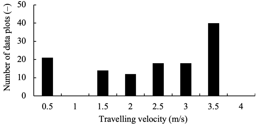
The mean value of the evaluated pitching angle was 0.19 rad in the non-rollover group and −0.092 rad in the rollover group, indicating a substantially smaller average for the latter. However, this does not imply that the evaluated pitch angle was consistently lower during rollover events. Rather, the lower mean value in the rollover group reflects a wide dispersion of data in both the positive and negative directions. This interpretation is supported by the variance–covariance matrices presented in Tables 4 and 5. Specifically, the variance of the evaluated pitching angle was 0.046 in the non-rollover group and a markedly greater value of 0.28 in the rollover group.
| Velocity | Vertical acceleration | Evaluated pitching angle | |
|---|---|---|---|
| Velocity | 1.1 | 0.020 | −0.0065 |
| Vertical acceleration | 0.020 | 1.9 | −0.044 |
| Evaluated pitching angle | −0.0065 | −0.044 | 0.046 |
| Velocity | Vertical acceleration | Evaluated pitching angle | |
|---|---|---|---|
| Velocity | 0.35 | 0.90 | −0.17 |
| Vertical acceleration | 0.90 | 66 | 2.5 |
| Evaluated pitching angle | −0.17 | 2.5 | 0.28 |
Based on the variance–covariance matrices presented in Tables 4 and 5, a discriminant function using the Mahalanobis distance was derived, as shown in Eq. (7) (0 < v ≦ 4.0).
| (7) |
Where C denotes the discriminant threshold. To determine an appropriate value of C, a sensitivity–specificity curve was constructed, as illustrated in Fig. 7.

As shown in Fig. 7, the intersection point of the two curves occurred at C = 3. Accordingly, the discriminant function for pitching rollovers was finalised as given in Eq. (8).
| (8) |
Figure 8 presents the simulation results for tractor behaviour on surfaces with lateral inclinations.

In Fig. 8, the blue circles represent non-rollover cases, whereas the red squares indicate rollover events. A total of 676,436 data points were simulated, of which 80 corresponded to rollover cases and 676,356 to non-rollover cases. The maximum and minimum values for each variable, along with the centroid (mean) values of the non-rollover and rollover groups, are summarised in Table 6.
| Velocity (m/s) | Vertical acceleration (m/s2) | Evaluated rolling angle (rad) | |
|---|---|---|---|
| Maximum | 4.0 | 48.4 | 5.1 |
| Minimum | 0.5 | −26.9 | −3.0 |
| Mean of the non-rollover group | 1.5 | −0.0028 | 0.061 |
| Mean of the rollover group | 2.2 | −4.4 | 0.50 |
The average velocity observed in the non-rollover group was approximately 1.5 m/s, which matched the overall mean velocity of the dataset. In contrast, the rollover group exhibited a higher mean velocity of 2.2 m/s, which closely corresponds to the average test velocity of 2.25 m/s. The distribution of rolling rollover occurrences across different velocity levels is illustrated in Fig. 9.

Unlike the pitching rollover data, the rolling rollover events were more evenly distributed across the entire range of tested velocities. Compared with pitching rollovers, it was more clearly found that velocity did not significantly affect rollovers.
3.1.2.2. Evaluated rolling angleIn contrast to the results observed in the pitching rollover simulations, the mean evaluated rolling angle in the non-rollover group was smaller than that in the rollover group. This difference can be attributed to the simulation conditions for lateral inclination, which involved terrain sloping unidirectionally from the left wheel contact point to the right. Consequently, the simulation reproduced only clockwise-rolling rollovers when viewed from the front of the tractor. This modelling approach was based on the assumption that because the centre of gravity of the tractor model was positioned at the midpoint of the wheel track, the dynamic response would be symmetric for clockwise and anticlockwise rollovers. Therefore, simulating a single direction was deemed sufficient.
Given that clockwise rotation was defined as positive in the simulation, the evaluated rolling angles in the rollover group simulated large positive values. Accordingly, if anticlockwise rollover data had been included, the mean evaluated angle for the rollover group would likely have been smaller, which would be more consistent with the trend observed in the pitching rollover simulations.
3.1.2.3. Results of discriminant analysisThe variance-covariance matrices for each group are shown in Tables 7 and 8.
| Velocity | Vertical acceleration | Evaluated rolling angle | |
|---|---|---|---|
| Velocity | 1.2 | −0.0026 | 0.024 |
| Vertical acceleration | −0.0026 | 1.7 | 0.014 |
| Evaluated rolling angle | 0.024 | 0.014 | 0.016 |
| Velocity | Vertical acceleration | Evaluated rolling angle | |
|---|---|---|---|
| Velocity | 1.4 | 0.16 | −0.0010 |
| Vertical acceleration | 0.16 | 14 | −0.067 |
| Evaluated rolling angle | −0.0010 | −0.067 | 0.0010 |
Based on these results, a discriminant function employing the Mahalanobis distance was formulated, as shown in Eq. (9).
| (9) |
In this case, the absolute value of the rolling evaluated angle was used because the dynamic behaviour of the tractor does not differ between the clockwise and anticlockwise roll directions (i.e. positive and negative values).
The threshold for the discriminant function was determined using the sensitivity–specificity curve, which balances sensitivity and specificity. This curve is shown in Fig. 10.

The intersection of the two curves indicated a threshold value of C = 0. Accordingly, the discriminant function for rolling rollover was established as shown in Eq. (10), valid for the velocity range 0 < v ≤ 4.0.
| (10) |
Table 9 presents the classification results obtained using the discriminant function (i.e. the rollover prediction equation) for pitching rollovers. Both the classification specificity and recall of the pitching rollover prediction were 96.4 %, with a misclassification rate of 3.6 %.
| Non-rollover data | Rollover data | |
|---|---|---|
| Non-rollover prediction |
1,315,033 (96.4 %) |
6 (3.6 %) |
| Rollover prediction |
49,317 (3.6 %) |
159 (96.4 %) |
Table 10 presents the classification results obtained using the discriminant function (i.e. the rollover prediction equation) for rolling rollovers.
| Non-rollover data | Rollover data | |
|---|---|---|
| Non-rollover prediction |
672,861 (99.5 %) |
0 (0 %) |
| Rollover prediction |
3,495 (0.5 %) |
80 (100 %) |
The classification specificity for the non-rollover group was 99.5 %, whereas recall for the rollover group was 100 %. The misclassification rate was 0 % for the rollover cases and 0.5 % for the non-rollover cases.
3.2.2. Prediction lead timeThe evaluated angle, which was used as an explanatory variable in the rollover prediction equation, was calculated using an integration interval of 0.3 s. This setting was intended to enable rollover prediction at least 0.3 s before the actual event.
To clarify the model’s actual prediction lead time, the developed equation was applied to the simulation dataset to determine how far in advance a rollover could be predicted under various conditions.
The validation results are summarised in Table 11. For each rollover event, the time at which the prediction equation first exceeded the threshold within the 1-second window preceding the rollover was recorded. The moment of rollover was defined as 0 s and the prediction times were expressed as negative values. On average, the first prediction occurred 0.88 s before pitching rollovers and 0.53 s before rolling rollovers.
| Terrain inclination angle (°) | Velocity (m/s) | Tpitch *1 (s) | Troll *2 (s) |
|---|---|---|---|
| 0 | 0.5 | – | – *3 |
| 1.0 | – | – | |
| 1.5 | – | – | |
| 2.0 | – | – | |
| 2.5 | – | – | |
| 3.0 | −1.00 | – | |
| 3.5 | −0.93 | – | |
| 4.0 | – | – | |
| 5 | 0.5 | – | – |
| 1.0 | – | −0.46 | |
| 1.5 | – | – | |
| 2.0 | – | – | |
| 2.5 | – | – | |
| 3.0 | −1.00 | – | |
| 3.5 | −0.98 | – | |
| 4.0 | – | – | |
| 10 | 0.5 | – | −0.61 |
| 1.0 | – | −0.91 | |
| 1.5 | – | −0.69 | |
| 2.0 | – | −0.55 | |
| 2.5 | – | −0.52 | |
| 3.0 | −1.00 | −0.47 | |
| 3.5 | −1.00 | −0.02 | |
| 4.0 | – | −0.42 | |
| 15 | 0.5 | – | −0.84 |
| 1.0 | – | −0.80 | |
| 1.5 | −0.76 | −0.62 | |
| 2.0 | −0.66 | −0.08 | |
| 2.5 | −0.69 | −0.43 | |
| 3.0 | −1.00 | −0.40 | |
| 3.5 | −1.00 | −0.64 | |
| 4.0 | – | −0.50 | |
| 20 | 0.5 | – | |
| 1.0 | – | ||
| 1.5 | −0.73 | ||
| 2.0 | −0.67 | ||
| 2.5 | – | ||
| 3.0 | – | ||
| 3.5 | – | ||
| 4.0 | – | ||
| Mean time | −0.88 | −0.53 | |
*1 Prediction time within 1.0 s before pitching rollover occurred.
*2 Prediction time within 1.0 s before rolling rollover occurred.
*3 Condition in which no rollover occurred.
In many cases, prediction equation output value initially exceeded the threshold, briefly dropped below it, and then exceeded it again immediately before the rollover. These fluctuations are interpreted as indicating a ‘grey zone’ or ‘marginal stability zone’, in which rollover is imminent but the vehicle is still marginally stable. If such fluctuations are recognised as early signs of a rollover, the timing data in Table 11 could be used to implement preventive interventions. For example, the average human cognitive response time in reaction to a warning system (from hazard perception to braking initiation) is approximately 0.7–0.8 s (Nakagawa et al., 2023; Olson et al., 1986). Therefore, the early prediction of pitching rollover could provide sufficient time to alert the operator and prevent an accident. Alternatively, if automatic control measures such as velocity adjustment, steering intervention, or posture stabilisation were applied directly to the vehicle, both pitching and rolling rollover incidents could potentially be avoided.
3.2.3. Data locality and overfittingThe discriminant functions for both pitching and rolling rollovers achieved exceptionally high specificity and recall. In general, when these values of a classification model—such as one derived from discriminant analysis—exceed 90 %, this raises potential concerns regarding underlying issues. These concerns include the possibility of using overly localised data and the occurrence of model overfitting.
3.2.3.1. Data localityWhen a dataset is highly localised, it represents only a narrow subset of the overall population that shares specific characteristics, which may artificially inflate classification accuracy.
However, the simulation in this study was carefully designed to span a broad and realistic range of conditions in terms of velocity, slope angle, and surface roughness.
The maximum test velocity of 4.0 m/s is relatively high for tractor operation and close to the recommended public road speed for tractors travelling on public roads. The maximum slope angle of 20 ° was selected to represent steep terrain, such as orchards or hilly and mountainous farmland. The highest level of surface roughness, labelled ‘very poor’, was designed to simulate rough environments such as grasslands or uneven natural surfaces. Conversely, the minimum test conditions—0.5 m/s velocity (representing low-speed tasks such as ridge shaping or embankment construction), 0 ° slope (flat terrain), and ‘very good’ surface roughness (similar to smooth concrete)—were included to reflect mild and stable operating scenarios. Notably, many rollover and fall incidents occur not during actual fieldwork but rather during field entry and exit, where such low-speed conditions are realistic.
Therefore, it can be concluded that the dataset used in this study was not overly localised and no issues related to data sampling bias were identified.
3.2.3.2. OverfittingThe precision rate was calculated to assess the possibility of overfitting. In cases of overfitting, a model typically achieves an abnormally high precision rate, meaning that it draws a decision boundary that perfectly separates positive and negative samples, even when such a separation may not be generalisable.
The precision rate for the pitching rollover prediction equation was 0.3 %, and that for the rolling rollover prediction equation was 2.2 %, indicating that overfitting did not occur.
In this study, simulated data were used instead of measured data, resulting in a noise-free dataset. In contrast, measured data often contain noise due to problems such as mislabelled samples (e.g. data labelled as rollover despite not reflecting an actual rollover, or data labelled as non-rollover despite the presence of unstable behaviour). Such labelling errors typically lead to misclassifications, which is why a classification accuracy exceeding 90 % is rare when using measured data.
Although it is theoretically possible to introduce artificial noise into the simulation, doing so would likely shift the decision boundary slightly—typically toward the non-rollover side—but would not substantially affect classification performance. Therefore, it was concluded that using simulated noisy data would offer limited practical benefits in the present context.
3.2.3.3. Conclusion regarding validity of prediction equationsIn summary, the use of simulation data was the primary factor contributing to the exceptionally high classification accuracy observed in this study. In discriminant analysis using noise-free data, high values for metrics such as sensitivity and specificity are expected. Furthermore, the clear distinction between rollover and non-rollover phenomena in the dataset further enhanced the classification performance of the model.
Therefore, no issues were identified regarding the validity of the high classification accuracy obtained from the discriminant analysis.
In this study, a behaviour-based RP estimation model was developed as a real-time risk assessment framework for tractor operating environments. The core of the model comprises rollover prediction equations, constructed using driving simulation data generated under a wide range of conditions. The main findings are summarised as follows.
1) The behaviour-based RP estimation model was developed by considering the nonlinear dynamic characteristics of tractor behaviour. The classification specificity and recall of the pitching rollover prediction equation were 96.4 % for non-rollover and rollover cases. For the rolling rollover prediction equation, the specificity was 99.5 % for non-rollover data, and the recall was 100 % for rollover data.
2) The average prediction lead time before rollover was 0.88 seconds for pitching rollovers and 0.53 seconds for rolling rollovers.
3) The discriminant analysis revealed no evidence of data locality. The precision rates were very low (0.3 % and 2.2 % for pitching and rolling, respectively), indicating that no overfitting occurred. This result is attributed to the use of noise-free simulation data.
4) Based on the above, the RP estimation models developed in both the first and second parts of this study were shown to possess sufficient accuracy and validity for practical use in real-time risk assessments.
In the phase of implementation of the framework as a system, following things must be considered. The acceleration data used for rollover prediction is supposed to be taken from accelerometer like IMU, and angular / angular acceleration need to be calculated by calculus of angular velocity sensed.
In addition, there are concern about integration drift because evaluated angles are calculated by double time integration. It is necessary to clarify the degree of drift occurred by calculus and affection level to rollover prediction as a validation for implementation. In the case drift is significant, some kind of filtering or bias correction method should be considered.
The authors thank Mr. Kai Kemmerling for language editing and constructive comments. This research received no external funding.
| Symbol | Description |
|---|---|
| a z | Vertical acceleration (m/s 2) |
| C | Discriminant threshold (–) |
| I | Behaviour-based risk point (RP) |
| p | Evaluated pitching angle (rad) |
| r | Evaluated rolling angle (rad) |
| T pitch | Prediction lead time for pitching rollover (s) |
| T roll | Prediction lead time for rolling rollover (s) |
| v | Travelling velocity (m/s) |
| γ | Matching rate (%) |
| e | Exponent of behaviour-based risk point (–) |
| τ | Output value of discriminant function (–) |
| φ | Pitching angle (rad) |
|
|
Pitching angle acceleration (rad/s 2) |
| θ | Rolling angle (rad) |
|
|
Rolling angle acceleration (rad/s 2) |
The authors declare no conflicts of interest.
(URLs on references were accessed on 6 July 2026.)