Abstract
Electrochemistry deals with the interrelationship between electrical and chemical energy. Various potentials appear in electrochemistry and pertain to one another in practical cells. Understanding the electrode potential is an important step in acquiring basic knowledge of electrochemistry and extending it to specific applications. This comprehensive paper outlines the fundamentals and related subjects of electrode potentials, including electrochemical cells and liquid junction potentials. Aqueous solution systems are ideal for connecting the theoretical background of electrode potentials to practical electrochemical measurements. Accordingly, the basic electrode chemistry in aqueous systems is described in this paper, as well as several advanced concepts introduced in recent studies.
1. Introduction
Electrode potential is the most salient and puzzling concept in electrochemistry.1–10 Although electric potentials in physics certainly underlie the concept of the electrode potential, the thermodynamic connection of the electrode potential to Gibbs energy represents the direction and scale of a redox reaction. A basic understanding of the electrode potential is necessary for constructing an appropriate electrochemical system and extending it to different applications.
Historically, the electrode potential has a variety of backgrounds, and its definition is somewhat ambiguous. This comprehensive, instructive paper summarizes the fundamental aspects of the electrode potential, mainly in the equilibrium state. Section 2 starts by defining the different types of electric potentials required in electrochemistry and describes the thermodynamic aspects connecting the Gibbs energy and the cell potential. Next, the electrochemical potential, which considers the chemical and electrical contributions to the total energy of a charged species, is introduced and connected to the Nernst equation. A basic description of the electrochemical cell is presented, as well as the definitions of related terms and tips for the use of coin cells. At the end of the section is a description of the junction potential at the interface of two electrolytic solutions, and information on salt bridges.
Section 3 covers aqueous solution systems, which provide good examples of the fundamental concepts and are ideal for connecting the theoretical background to practical electrochemical measurements. Information is provided on the basic electrode chemistry in aqueous systems, including the Pourbaix diagram, electrochemical window, practical reference electrode, and mixed potentials, as well as several advanced concepts introduced in recent studies. Detailed slides for each section are provided in the Supplementary Material.
2. Fundamentals
2.1 Inner, outer, and surface electric potentials
The electric potential of a charged species generally corresponds to work that brings it from the point at infinity to a specific point. Figures 1a and 1b summarizes the relationship between the inner, outer, and surface electric potentials and the Galvani and Volta potentials for metal M. The inner electric potential (ϕM) is the potential to bring a charged particle from the point at infinity (point O) to a specific point in the bulk of M (point B), and thus the difference between the two inner electric potentials (e.g., $\phi^{\text{M}_{1}}$ and $\phi^{\text{M}_{2}}$, where M1 and M2 are two different metals) provides the Galvani potential ($\varDelta \phi_{\text{M}_{1}}^{\text{M}_{2}}$). The outer electric potential (ψM) is a potential to bring a charged particle from the point of infinity (point O) to the surface of M (point A), and the difference between the two outer potentials ($\psi^{\text{M}_{1}}$ and $\psi^{\text{M}_{2}}$) is called the Volta potential ($\varDelta \psi_{\text{M}_{1}}^{\text{M}_{2}}$). The surface electric potential (χM) originates from the dipolar charge distribution at the surface of M. These three potentials are connected using Eq. 1; however, only ψM, which is the potential difference between two points in the same phase, is a measurable quantity.
| \begin{equation}
\phi^{\text{M}} = \psi^{\text{M}} + \chi^{\text{M}}
\end{equation}
| (1) |
The electrode potential can be regarded as the potential difference between a point in the solid conductor (M, e.g., metal) and another point in the electrolytic solution (S) (thus, the Galvani potential,
$\Delta \phi_{\text{S}}^{\text{M}}$) (Fig.
1c). The partial molar Gibbs energy of a charged species has chemical and electrical contributions (see electrochemical potential in Section 2.3). The Galvani potential is not directly measurable because the separation of chemical and electrical contributions is difficult when measuring the potential difference between two different phases.
5,11,12 If the potential difference between points in the same phase is measured in the equilibrium state, their chemical contributions are identical, and thus the potential difference is measurable. In practical measurements, the electrode potential is measured as a relative value by introducing an additional electrode (reference electrode), as explained in the following sections.
2.2 Thermodynamic background
When considering the following n-electron redox reaction (Eq. 2), the corresponding reaction Gibbs energy, ΔrG, is provided by Eq. 3 using the chemical potential, μi, and activity, ai, of two pairs of oxidants and reductants (Ox/Red and Ox′/Red′).
| \begin{equation}
\text{Ox} + \text{Red}' \rightleftharpoons \text{Red} + \text{Ox}'
\end{equation}
| (2) |
| \begin{align}
\Delta_{\text{r}}G & = \mu_{\text{Red}} + \mu_{\text{Ox${'}$}} - \mu_{\text{Ox}} - \mu_{\text{Red${'}$}}\\
& = (\mu_{\text{Red}}^{\circ} + \mu_{\text{Ox${'}$}}^{\circ} - \mu_{\text{Ox}}^{\circ} - \mu_{\text{Red${'}$}}^{\circ}) + RT\ln\frac{a_{\text{Red}}a_{\text{Ox${'}$}}}{a_{\text{Ox}}a_{\text{Red${'}$}}}\\
& = \Delta_{\text{r}}G^{\circ} + RT\ln Q
\end{align}
| (3) |
where
R,
T, and
Q are the gas constant, temperature, and reaction quotient, respectively. The superscript circle indicates that the quantity is in the standard state. Here, the coefficients of the terms in Eq. 2 are one for simplicity.
An important relationship between ΔrG and the cell potential, ε (the International Union of Pure and Applied Chemistry (IUPAC)13 recommends using the cell potential instead of the electromotive force, emf) for the corresponding electrochemical cell is introduced as follows (Eq. 4):
| \begin{equation}
\Delta_{\text{r}}G = -nF\varepsilon
\end{equation}
| (4) |
where
n and
F are the stoichiometric coefficients of the electrons in the reaction and the Faraday constant, respectively. The right side of Eq. 4 is obtained by considering the electrical work, which is the product of the charge (Faraday constant for one mole) and
ε, and corresponds to Δ
rG under a constant temperature and pressure. The following equation for the corresponding electrochemical cell is obtained by combining Eqs. 3 and 4.
| \begin{equation}
\varepsilon = \varepsilon^{\circ} - \frac{RT}{nF}\ln Q
\end{equation}
| (5) |
When Red′ and Ox′ in Eq. 2 are $\frac{1}{2}$H2(g) and H+(aq), respectively, in their standard states, Eq. 3 can be written as follows (Eq. 6):
| \begin{equation}
\Delta_{\text{r}}G = \Delta_{\text{r}}G^{\circ} + RT\ln\frac{a_{\text{Red}}}{a_{\text{Ox}}}
\end{equation}
| (6) |
Figure 2 shows the corresponding electrochemical cell, in which the working electrode potential is measured with respect to the reference electrode potential. The H+/H2 redox couple in the standard state is the universal reference electrode, known as the standard hydrogen electrode (SHE), and its standard electrode potential, E°, is zero at all temperatures (E°(H+/H2) = 0).13 Thus, ε in this case can be regarded as the electrode potential representing the half-cell reaction (Eq. 7) in question, and is simply called the electrode potential, E.
| \begin{equation}
\text{Ox} + ne^{-}\rightleftharpoons \text{Red}
\end{equation}
| (7) |
The half-cell reaction is written in the reduction direction. This is a practical way to define
E. From Eqs. 4 and 6, the following relationship is obtained (Eq. 8):
| \begin{equation}
E = E^{\circ} - \frac{RT}{nF}\ln\frac{a_{\text{Red}}}{a_{\text{Ox}}}
\end{equation}
| (8) |
where
E° is related to Δ
rG° by Δ
rG° = −
nFE°.
2.3 Electrochemical potential
The chemical and electrochemical potentials (μ and $\tilde{\mu }$) defined in Eqs. 9 and 10 are important quantities for introducing the electrode potential under a constant potential and temperature. The two terms contain the word “potential;” however, their unit is J mol−1 and is different from the unit of the electrode potential (V).
| \begin{equation}
\mu_{i} = \left(\frac{\partial G}{\partial n_{i}}\right)_{n_{j \neq i}} {}= \mu_{i}^{\circ} + RT\ln a_{i}
\end{equation}
| (9) |
| \begin{equation}
\tilde{\mu}_{i} = \mu_{i} + z_{i}F\phi = \mu_{i}^{\circ} + RT\ln a_{i} + z_{i}F\phi
\end{equation}
| (10) |
where
zi is the charge of the charged species and
ϕ is the inner potential of the phase (see Section 2.1) containing the charged species. The chemical potential is the partial molar Gibbs energy, and the electrochemical potential includes the electrostatic contribution for the charged species in addition to the chemical potential; the last term of Eq. 10 represents the work of moving the ion from infinity to a certain point in the solution. Considering the case of Eq. 6, the chemical potentials of the ions in the solution (Ox and Red) and the electrons in the metal (e) are expressed as follows (Eqs. 11-1, 11-2, and 11-3):
| \begin{equation}
\tilde{\mu}_{\text{Ox}} = \mu_{\text{Ox}} + z_{\text{Ox}}F\phi^{\text{S}} = \mu_{\text{Ox}}^{\circ} + RT\ln a_{\text{Ox}} + z_{\text{Ox}}F\phi^{\text{S}}
\end{equation}
| (11-1) |
| \begin{equation}
\tilde{\mu}_{\text{Red}} = \mu_{\text{Red}} + z_{\text{Red}}F\phi^{\text{S}} = \mu _{\text{Red}}^{\circ} + RT\ln a_{\text{Red}} + z_{\text{Red}}F\phi^{\text{S}}
\end{equation}
| (11-2) |
| \begin{equation}
\tilde{\mu}_{\text{e}} = \mu_{e}^{\circ} - F\phi^{\text{M}}
\end{equation}
| (11-3) |
where
ϕS and
ϕM are the inner electric potentials of the solution and metal, respectively, and electroneutrality requires the following relationship:
zOx =
n +
zRed. Here, the activity of the electron in M is one, and thus,
$\mu_{\text{e}} = \mu_{e}^{ \circ }$. The following equation holds in the equilibrium state (Eq. 12):
| \begin{equation}
\tilde{\mu}_{\text{Ox}} + n\tilde{\mu}_{\text{e}} = \tilde{\mu}_{\text{Red}}
\end{equation}
| (12) |
Equations 11-1, 11-2, 11-3, and 12 yield the following relationship (Eq. 13):
| \begin{align}
&(\mu_{\text{Ox}}^{\circ} + RT\ln a_{\text{Ox}} + z_{\text{Ox}}F\phi^{\text{S}}) + n(\mu_{e}^{\circ} - F\phi^{\text{M}}) \notag\\
&\quad= \mu_{\text{Red}}^{\circ} + RT\ln a_{\text{Red}} + z_{\text{Red}}F\phi^{\text{S}}
\end{align}
| (13) |
When the electrode potential,
E, is defined as occurring at the interface between the metal and the solution, it can be expressed as follows (Eq. 14) from Eq. 13:
| \begin{align}
E & = \phi^{\text{M}} - \phi^{\text{S}}\\
& = -\frac{\mu_{\text{Red}}^{\circ} - \mu_{\text{Ox}}^{\circ} - n\mu_{\text{e}}^{\circ}}{nF} - RT\ln\frac{a_{\text{Red}}}{a_{\text{Ox}}}\\
& = E^{\circ} - \frac{RT}{nF}\ln\frac{a_{\text{Red}}}{a_{\text{Ox}}}
\end{align}
| (14) |
Here, Eq. 14 is derived by considering only a half-cell reaction, and it is known as the Nernst equation. Equation 8 is derived in a different manner, but has the same form as Eq. 14 and can be converted to a more practical form (Eq. 15) by separating the activity coefficient and the concentration and introducing the formal potential,
E°′:
| \begin{align}
E & = E^{\circ} - \frac{RT}{nF}\ln\frac{a_{\text{Red}}}{a_{\text{Ox}}}\\
& = E^{\circ} - \frac{RT}{nF}\ln\frac{\gamma_{\text{Red}}}{\gamma_{\text{Ox}}} - \frac{RT}{nF}\ln\frac{c_{\text{Red}}}{c_{\text{Ox}}}\\
& = E^{\circ\prime} - \frac{RT}{nF}\ln\frac{c_{\text{Red}}}{c_{\text{Ox}}}
\end{align}
| (15) |
The selected E° values at 25 °C are listed in Table 1.14 Although the H+/H2 couple (SHE) is defined as the reference for all the E° values, more convenient redox couples with a high reversibility are practically used as reference electrodes (details on practical reference electrodes are provided below). The ionic species in the list are assumed to be in an aqueous solution, which means that E° can be different in other solvents. The oxidizing power of the species on the left side decreases from high to low E°; F2 in F2/F− is the strongest oxidizer, and Li in Li+/Li is the strongest reducer in the list (Table 1).
Table 1. Standard electrode potentials of selected redox couples.
| Half-cell reactions |
E° |
| F2 + 2e− ⇌ 2F− |
+2.87 |
| Ce4+ + e− ⇌ Ce3+ |
+1.72 |
| MnO4− + 8H+ + 5e− ⇌ Mn2+ + 4H2O |
+1.51 |
| Cl2 + 2e− ⇌ 2Cl− |
+1.36 |
| Cr2O72− + 14H+ + 6e− ⇌ 2Cr3+ + 7H2O |
+1.36 |
| O2 + 4H+ + 4e− ⇌ 2H2O |
+1.23 |
| Br2 + 2e− ⇌ 2Br− |
+1.07 |
| Ag+ + e− ⇌ Ag |
+0.80 |
| Hg22+ + 2e− ⇌ 2Hg |
+0.80 |
| Fe3+ + e− ⇌ Fe2+ |
+0.77 |
| Cu2+ + 2e− ⇌ Cu |
+0.34 |
| AgCl + e− ⇌ Ag + Cl− |
+0.22 |
| 2H+ + 2e− ⇌ H2 |
0 |
| Pb2+ + 2e− ⇌ Pb |
−0.13 |
| Sn2+ + 2e− ⇌ Sn |
−0.14 |
| Fe2+ + 2e− ⇌ Fe |
−0.44 |
| Zn2+ + 2e− ⇌ Zn |
−0.76 |
| Al3+ + 3e− ⇌ Al |
−1.68 |
| Mg2+ + 2e− ⇌ Mg |
−2.36 |
| Na+ + e− ⇌ Na |
−2.71 |
| Ca2+ + 2e− ⇌ Ca |
−2.84 |
| K+ + e− ⇌ K |
−2.93 |
| Li+ + e− ⇌ Li |
−3.05 |
2.4 Electrochemical cell
In electrochemical measurements, the electrode to be measured is called the working electrode (sometimes the indicator or test electrode) against the reference electrode. The electrode potential can be measured in a two-electrode cell when no current is flowing (Fig. 3a). However, a stable reference electrode (non-polarized) is necessary to correctly measure the potential of the working electrode under a current flow; thus, another electrode, called the counter electrode (or auxiliary electrode), is required. In such an arrangement, called a three-electrode cell (Fig. 3b), the current passes between the working and counter electrodes, and the reference electrode potential remains constant. When an ohmic drop occurs in the solution, iRs (i and Rs denote the current and solution resistance, respectively), and is not negligible under a current flow, the working electrode potential cannot be correctly measured. The ohmic drop can be minimized by placing the reference electrode near the working electrode. Although the use of Luggin-Haber capillary further reduces this contribution,15 the uncompensated potential drop still remains and needs to be corrected by instrumental techniques such as a positive feedback compensation scheme.16
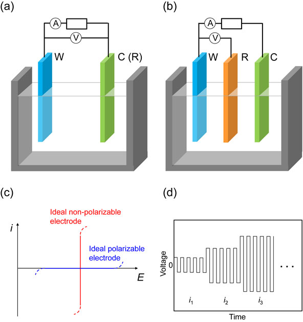
The open-circuit potential (or rest potential) indicates the potential of a working electrode when no external current is flowing (see Section 3.4 for the open circuit potential under mixed potential). If no charge transfer (no redox reaction) occurs on a certain electrode in an electrolytic solution polarized from the open-circuit potential, the electrode–solution interface acts as a capacitor. Such an electrode is referred to as an ideal polarizable electrode and is used to investigate the double-layer behavior. On the other hand, an ideal non-polarizable electrode has an infinitely high exchange current density, and its potential does not change upon the passage of a current, indicating a potential determined by the Nernst equation. This behavior is preferable for use as the reference electrode. Figure 3c shows the relationship between the current and the potential for the ideal polarizable and non-polarizable electrodes.
Particular attention should be paid to electrochemical measurements using coin cells. Two-electrode coin cells are commonly used in batteries owing to their convenience. The solution resistance in coin cells can be minimized by placing the two electrodes close to each other (using a thin separator with a thickness of a few tens of micrometers) and increasing the electrode area. The performance of an electrode active material is often evaluated using a half-cell test with a metal counter electrode. For example, a lithium metal counter electrode in an electrolytic solution containing a lithium salt also works as a reference electrode in a two-electrode configuration in the form of Li+/Li. Although discussions are often based on the assumption that the Li+/Li equilibrium potential holds under a current flow, its non-zero charge transfer resistance certainly induces polarization (negatively during lithium metal deposition and positively during lithium metal dissolution). Consequently, the working electrode potential appears to be higher during delithiation and lower during lithiation (polarization also depends on various parameters such as the electrolyte and temperature). Thus, careful interpretation is required for measurements using coin cells, particularly at high current densities. Metal deposition/dissolution cycle tests for a Li/Li symmetric cell can provide useful information on the degree of polarization of the lithium metal electrode (Fig. 3d);17 polarization (response of voltage) is evaluated by increasing the direct current (DC) (i1 < i2 < i3 < ⋯) stepwise and repeating the deposition/dissolution up to a specific cycle number required in measurements where the Li metal counter electrode is used. Electrochemical impedance spectroscopy can provide similar information.
2.5 Liquid junction potential
The liquid junction potential appears at the junction of two different electrolytic solutions. When both the cations and anions diffuse through the junction by the concentration gradient, the difference in their mobilities causes a charge separation, as shown in Fig. 4a.2,10 The liquid junction potential compensates for this charge separation (and thus this type of liquid junction potential is called a diffusion potential); it forms to slow down the faster ions and speed up the slower ions to satisfy charge neutrality, as shown in Fig. 4b. The liquid junction potential is defined as the Galvani potential between the right and left phases (the inner potential of the right phase with respect to that of the left phase in the case shown in Fig. 4b). Mass transfer in electrolytic solutions based on ion diffusion and migration is described by the Nernst-Planck equation (Eq. 16) by neglecting convection as follows:
| \begin{equation}
J = -D\left(\frac{\text{d}c}{\text{d}x}\right) - \frac{z}{|z|}uc\left(\frac{\text{d}\phi}{\text{d}x}\right)
\end{equation}
| (16) |
where
J,
D,
c, and
u are the flux, diffusion coefficient, concentration, and mobility, respectively. This equation contains two derivative terms; thus, it is difficult to obtain an analytical solution without assumptions. Two different assumptions provide two different approximate junction potential equations. When the concentration gradient of an ion (
i) is assumed to be constant everywhere in the junction, the following Henderson equation is obtained (Eq. 17):
| \begin{equation}
\Delta\phi = -\cfrac{\displaystyle\sum\nolimits_{i}|z_{i}|\cfrac{u_{i}}{z_{i}}(c_{i,d} - c_{i,0})}{\displaystyle\sum\nolimits_{i}|z_{i}|u_{i}(c_{i,d} - c_{i,0})}\frac{RT}{F}\ln\left[\frac{\displaystyle\sum\nolimits_{i}(|z_{i}|u_{i}c_{i,d})}{\displaystyle\sum\nolimits_{i}(|z_{i}|u_{i}c_{i,0})}\right]
\end{equation}
| (17) |
The Goldman equation (Eq. 18) is obtained by assuming that the electric field is constant in the junction between 1 : 1 electrolytes (
j represents cations and
k represents anions):
| \begin{equation}
\Delta\phi = -\frac{RT}{F}\ln\left[\frac{\displaystyle\sum\nolimits_{j}(\omega_{j}c_{j,d}) + \displaystyle\sum\nolimits_{k}(\omega_{k}c_{k,0})}{\displaystyle\sum\nolimits_{j}(\omega_{j}c_{j,0}) + \displaystyle\sum\nolimits_{k}(\omega_{k}c_{k,d})}\right]
\end{equation}
| (18) |
Both equations indicate that a concentrated solution with ions of nearly equivalent mobility can minimize the liquid junction potential to another solution with a low concentration. Examples of such salts are KCl and KNO
3 in aqueous solutions and tetraethylammonium picrate in nonaqueous solutions. A typical intermediate salt bridge for an aqueous solution is prepared by gelling KCl with agar in a glass tube and using it to connect the two solutions as shown in Fig.
2. A liquid junction potential less than a few millivolts is negligible in practical experiments because phenomena within such errors is often observed in electrochemical measurements.
A prominent topic in this area is the use of an ionic liquid salt bridge proposed by Kakiuchi and coworkers.18,19 A hydrophobic ionic liquid ([C][A]) and an aqueous solution form a two-phase system. The liquid junction potential between these two phases ($\Delta\phi_{\text{IL}}^{\text{W}} $) is thermodynamically determined by the distribution potential (Eq. 19) and thus the ionic liquid salt bridge is distinct from the previously known ones, such as the KCl salt bridge, for which the phase-boundary potentials are determined by the non-thermodynamic diffusion potential.
| \begin{equation}
\Delta\phi_{\text{IL}}^{\text{W}} = \frac{1}{2}({\Delta\phi(\text{C${^{+}}$})^{\circ}}_{\text{IL}}^{\text{W}} + {\Delta\phi(\text{A${^{-}}$})^{\circ}}_{\text{IL}}^{\text{W}}) + \frac{RT}{2F}\ln\frac{\gamma_{\text{A${^{-}}$}}^{\text{W}}\gamma_{\text{C${^{+}}$}}^{\text{IL}}}{\gamma_{\text{C${^{+}}$}}^{\text{W}}\gamma_{\text{A${^{-}}$}}^{\text{IL}}}
\end{equation}
| (19) |
where
${\Delta\phi(\text{C}^{ + })^{ \circ }}_{\text{IL}}^{\text{W}}$ and
${\Delta\phi(\text{A}^{ - })^{ \circ }}_{\text{IL}}^{\text{W}}$ are the standard ion transfer potentials of the cations (C
+) and anions (A
−), respectively, and γ corresponds to the activity coefficient of the ions in the aqueous (W) or ionic liquid (IL) phases. Two other potentials, diffusion and mixed potentials caused by the mobility difference between the C
+ and A
− ions in the aqueous phase, need to be considered in practical cases, but these contributions can be minimized by using an ionic liquid consisting of cations and anions with similar mobilities, as in the case of the KCl salt bridge. Fast response, high stability, and low contamination are the advantages of ionic liquid salt bridges. Although the experimentally obtained junction potential between the 1-methyl-3-octylimidazolium bis(trifluoromethanesulfonyl)amide ([C
8C
1im][TFSA]) ionic liquid and HCl, LiCl, NaCl, and KCl solutions remained constant within ±1 mV over the change in the concentration from 1.0 × 10
−4 to 0.2 mol dm
−3, a deviation from the constant value was observed at low concentrations (<10
−4 mol dm
−3).
20 This is attributed to the diffusion potential caused by the lower mobility of [C
8C
1im]
+ compared to that of [TFSA]
−. A more stable salt bridge was constructed with [P
444(201)][TFSA] ([P
444(201)]
+ = tributyl(2-methoxyethyl)phosphonium) owing to the similar mobilities of [P
444(201)]
+ and [TFSA]
−, exhibiting a constant phase boundary potential with the aqueous alkali metal iodide solutions down to a low concentration of ∼10
−6 mol dm
−3.
21
The liquid junction potential in highly concentrated aqueous solutions was discussed in a recent study.22 Taking the equilibrated LiFePO4/FePO4 couple as an example of a Li+-insertion electrode, the difference in the electrode potentials in a highly concentrated LiCl aqueous solution (e.g., 18 mol kg−1 LiCl aq.) and reference electrolyte (e.g., 1 mol kg−1 LiCl aq.) (ΔE) is expressed by three different contributions (Eq. 20):
| \begin{equation}
\Delta E = \Delta E_{\text{N}}^{c} + \Delta E_{\text{N}}^{\gamma} + \Delta E_{\text{LJP}}
\end{equation}
| (20) |
where the first two Nernstian contributions (
$\Delta E_{\text{N}}^{c}$ and
$\Delta E_{\text{N}}^{\gamma }$) are associated with the changes in the concentration and activity coefficient, and the last contribution (Δ
ELJP) is the liquid junction potential. Because
$\Delta E_{\text{N}}^{c}$ can be calculated from the Nernst equation, the plot of
$\Delta E - \Delta E_{\text{N}}^{c}$ against the molality of a lithium salt is a good indicator to estimate
$\Delta E_{\text{N}}^{\gamma } + \Delta E_{\text{LJP}}$. The diffusion potential calculated by the Henderson equation suggests a negligible contribution, but the two assumptions regarding the activity and mobility of the ions in the Henderson equation are not valid in highly concentrated solutions. The assumption that the activities of the ions are equal to the mean activity of the salt and the transport numbers for the cations and anions are independent of the molality can provide another simple approximation: the liquid junction potential to a situation where a junction is formed between two solutions of common ions in different concentrations and the ions move across the junction to a lower concentration yields a value over 100 mV in the case between 1.0 and 18 mol kg
−1 LiCl solutions. Although the assumptions applied here may not be completely correct, it is obvious that discussions about the redox potential in highly concentrated solutions must consider the junction potential.
3. Aqueous Systems
3.1 Potential–pH diagram
In electrochemical systems that use aqueous solutions as electrolytes, the pH ($ = - \log_{10}a_{\text{H}^{ + }}$) of the solution is often responsible for the potential-determining reaction and the equilibrium electrode potential. For example, zinc ions are dissolved as Zn2+ ions (more correctly, hydrated Zn(OH2)62+) in acidic solutions but precipitate mainly as Zn(OH)2 in neutral solutions, and [Zn(OH)4]2− is the main dissolved species in alkaline solutions. The redox reaction of zinc ions in acids is as follows:
| \begin{equation}
\text{Zn$^{2+}$} + 2\text{e}^{-}\rightleftharpoons \text{Zn}
\end{equation}
| (21) |
and its electrode potential at 25 °C can be derived using the Nernst equation:
| \begin{align}
E_{\text{acid}} & = E_{\text{acid}}^{\circ} - \frac{RT}{2F}\ln \frac{a_{\text{Zn}}}{a_{\text{Zn${^{2+}}$}}} = E_{\text{acid}}^{\circ} + \frac{RT}{2F}\ln [\text{Zn$^{2+}$}]\\
& = E_{\text{acid}}^{\circ} + 0.0296\log [\text{Zn$^{2+}$}]
\end{align}
| (22) |
where it is assumed that “the activity is equal to the concentration, and the activity of the solid is one.” However, the reduction of zinc ions in alkaline solutions is as follows:
| \begin{equation}
\text{[Zn(OH)$_{4}$]$^{2-}$} + 2\text{e}^{-}\rightleftharpoons \text{Zn} + \text{4OH$^{-}$}
\end{equation}
| (23) |
and the electrode potential at 25 °C is as follows:
| \begin{align}
E_{\text{base}} & = E_{\text{base}}^{\circ} - \frac{RT}{2F}\ln \frac{a_{\text{Zn}} \cdot a_{\text{OH${^{-}}$}}^{4}}{a_{\text{[Zn(OH)${_{4}}$]${^{2-}}$}}} = E_{\text{base}}^{\circ} + \frac{RT}{2F}\ln \frac{[\text{Zn(OH)$_{4}^{2-}$}]}{a_{\text{OH$^{-}$}}^{4}}\\
& = E_{\text{base}}^{\circ} + 0.0295\log[\text{Zn(OH)$_{4}^{2-}$}] + 0.118(14 - \text{pH})
\end{align}
| (24) |
When comparing Eqs. 22 and 24, it can be seen that in acidic solutions, the electrode potential is independent of the pH. However, in alkaline solutions, the electrode potential decreases as the pH increases. Such electrode potential behavior indicates that the pH of the solution must be considered when studying electrochemical reactions in aqueous solutions.
Therefore, a diagram showing the dissolved ionic or chemical species of the element of interest on a two-dimensional plane of the electrode potential vs. pH is a good guide for electrochemical reactions in aqueous solutions. The potential–pH diagram is also known as the Pourbaix diagram, named after the Belgian chemist Marcel Pourbaix (1904–1998). Initially, Pourbaix used the potential–pH diagram to study corrosion; today, potential–pH diagrams are available for almost all the elements. In addition, potential–pH diagrams for multiple elements can be drawn using commercial software with thermodynamic data.
For example, a potential–pH diagram for zinc is shown in Fig. 5.23 The two dashed lines in the figure are the standard potentials for the oxygen evolution and hydrogen evolution reactions and represent the theoretical stable region (potential window) of water. Potential windows are discussed in detail in the next section. The diagram can be divided into five regions where Zn2+, Zn(OH)2, [HZnO2]−, [Zn(OH)4]2−, and Zn are stable. The boundary line represents the equilibrium conditions (pH and electrode potentials), and the position of the boundary line may vary with the concentration of dissolved ion species (1.0 × 10⁻⁶ mol dm−3 in Fig. 5). Line (A) is a horizontal line, indicating that the potential-determining reaction is unaffected by changes in the pH, as shown in Eq. 21. Lines (E)–(G) have negative slopes because the electrode potential is affected by the pH. Lines (B)–(D) are not redox reactions (the oxidation number of zinc remains at +2) but are dissolution-precipitation reactions, and there is no change in the electrode potential.
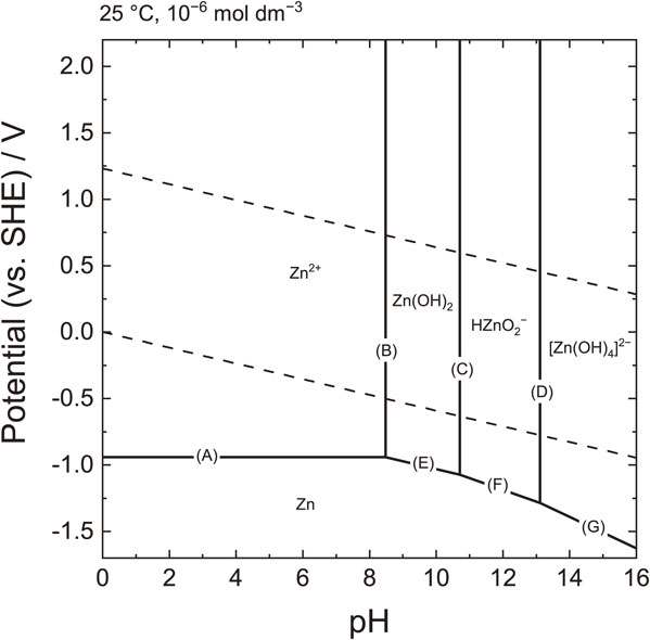
The line types can be summarized as follows:
-
(1)
Two different species of the element of interest (solid or dissolved), protons involved, but no electron transfer: vertical line
-
(2)
Two different species of the element of interest (solid or dissolved), electrons involved, but no protons involved: horizontal line
-
(3)
Two different species of the element of interest (solid or dissolved), protons and electrons are involved: oblique line
A simple potential–pH diagram can be derived relatively easily from thermodynamic data, but the calculation is complicated when multiple elements are considered. Density functional theory (DFT) calculations have recently been used to determine the total energy of chemical species, and the results provided the basis for the potential–pH diagram. However, when multiple elements are considered in DFT first-principles electronic structure calculations, numerous computational resources are required to search for candidate compounds. In recent years, algorithms for this purpose have been improved to search for convex hulls of stable candidate compounds. Many algorithms have been published that can be used together with the results of DFT calculations. For example, Fig. 6 shows a potential–pH diagram for zinc and manganese drawn by the Pourbaix diagram implemented in the Materials Project.24–26 As shown, the zinc and manganese compounds are drawn in a complex manner. An example code for drawing a Pourbaix diagram is provided in the Supporting Information.
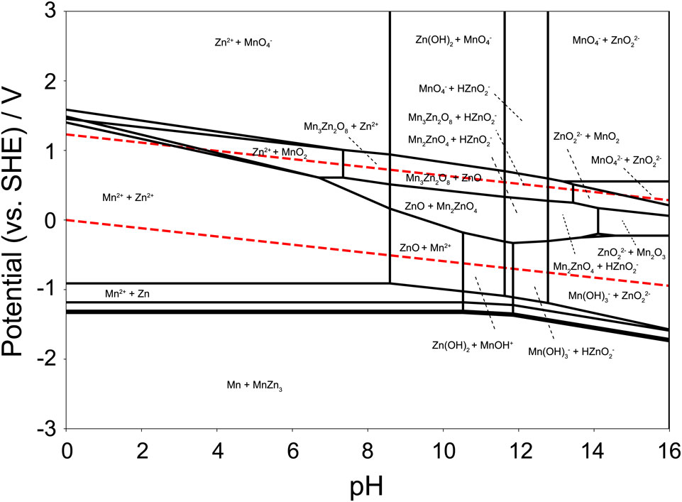
The potential–pH diagram shows the region of the pH and potential where a compound is stable, and acts as a guide map when considering the electrochemistry of aqueous solutions.
3.2 Electrochemical window
In an aqueous solution, oxygen and hydrogen evolution reactions occur when the electrode potentials are high and low, respectively. Therefore, the upper and lower limits of the electrode potential that can be applied in an electrochemical cell using an aqueous solution are determined by both reactions; this potential range is called the electrochemical window (or potential window). In the potential–pH diagram for zinc, the region sandwiched between the two dashed lines corresponds to the electrochemical window. The oxygen evolution reaction in acidic and basic solutions is described by Eqs. 25 and 26 as follows:
| \begin{equation}
\text{2H$_{2}$O} \rightleftharpoons \text{O$_{2}$} + \text{4H$^{+}$} + 4\text{e}^{-}
\end{equation}
| (25) |
| \begin{equation}
\text{4OH$^{-}$} \rightleftharpoons \text{O$_{2}$} + \text{2H$_{2}$O} + 4\text{e}^{-}
\end{equation}
| (26) |
The hydrogen evolution reaction in acidic and basic solutions is described by Eqs. 27 and 28 as follows:
| \begin{equation}
\text{2H$^{+}$} + 2\text{e}^{-} \rightleftharpoons \text{H$_{2}$}
\end{equation}
| (27) |
| \begin{equation}
\text{2H$_{2}$O} + 2\text{e}^{-} \rightleftharpoons \text{H$_{2}$} + \text{2OH$^{-}$}
\end{equation}
| (28) |
As shown in Eqs. 25–28, the potential-determining reactions depend on the pH; thus, the two dashed lines have negative slopes.
In practice, some overpotentials are required to allow the oxygen evolution and hydrogen evolution reactions to proceed, resulting in a larger potential window than the thermodynamic theoretical potential window of 1.23 V (25 °C). Owing to these overpotentials, a nominal voltage of 2.1 V is possible in lead–acid batteries.27 Conversely, water electrolysis, in which clean hydrogen can be produced, requires a voltage of 2 V or higher.
As a new topic regarding the potential window of aqueous solutions, research on the use of aqueous electrolytes in inexpensive and environmentally benign rechargeable batteries is gaining momentum. Compared with organic solvents and ionic liquids, aqueous solutions have a narrower potential window, which limits the operating voltage of the battery. Research on new aqueous electrolytes that achieve a wide potential window is underway by modifying the additives, electrolyte salts, and electrolyte concentration.28–31 Clarification of the origin of the wide potential window has been attempted by DFT calculations and analysis of the electrode/electrolyte interface, although no unified conclusion has been reached. However, it should be noted that the gap between the HOMO and LUMO obtained from the DFT calculations of water is extremely large (8.7 eV) and far from the actual thermodynamic data; therefore, the potential window cannot simply be obtained from the gap between the HOMO and LUMO.32
Although not discussed in detail in this paper, the potential window is important not only from a thermodynamic viewpoint but also from a kinetic viewpoint. Even if the electrode potential is outside the thermodynamic potential window, the kinetics of water decomposition may be sufficiently slow, in which case the aqueous electrolyte can be treated as apparently stable. Sufficiently slow kinetics is a state in which water molecules are unlikely to be supplied near the electrode, which is thought to be realized by the formation of a surface electrolyte interphase (SEI), which is a decomposition product of the electrolyte, or a local structure near the electrode in which water molecules are unlikely to be released.33
3.3 Practical reference electrodes
The reference electrode should be an ideal nonpolarizable electrode with a large exchange current density such that a small polarization allows a large current flow. The primary reference electrode used in aqueous solutions is the standard hydrogen electrode (SHE). However, SHE is an ideal device that cannot be realized experimentally. Therefore, reversible hydrogen electrodes (RHEs), which depend on the solution pH, are widely used.
The Nernst equation in Eq. 27 is as follows:
| \begin{align}
E(\text{RHE}) & = E^{\circ} - \frac{RT}{2F}\ln \left(\frac{p_{\text{H${_{2}}$}}/p^{\circ}}{a_{\text{H${^{+}}$}}^{2}}\right)\\
& = -2.303\frac{RT}{2F}\left(\log \frac{p_{\text{H${_{2}}$}}}{p^{\circ}} + \text{2pH}\right)
\end{align}
| (29) |
The applied convention is that the standard potential of hydrogen
E°(H
2/H
+) = 0 at all temperatures. Although the hydrogen partial pressure should strictly consider the effects of water vapor and hydrostatic pressure, the error at 25 °C is only approximately 1 mV; thus, it is usually not necessary to take this into account. In addition, the difference between the standard pressure defined by the IUPAC (10
5 Pa) and 1 atm (101,325 Pa) is approximately 0.1 mV.
Generally, an electrode of the second type, as shown below, is used as the reference electrode.
Silver–silver chloride electrode Ag/AgCl
| \begin{equation}
\text{AgCl} + \text{e}^{-} \rightleftharpoons \text{Ag} + \text{Cl$^{-}$}
\end{equation}
| (30) |
Mercury–mercury(I) chloride electrode (calomel electrode) Hg/Hg
2Cl
2
| \begin{equation}
\text{Hg$_{2}$Cl$_{2}$} + 2\text{e}^{-} \rightleftharpoons \text{2Hg} + \text{2Cl$^{-}$}
\end{equation}
| (31) |
Mercury–mercury(I) sulfate electrode Hg/Hg
2SO
4
| \begin{equation}
\text{Hg$_{2}$SO$_{4}$} + 2\text{e}^{-} \rightleftharpoons \text{2Hg} + \text{SO$_{4}^{2-}$}
\end{equation}
| (32) |
Mercury–mercury(II) oxide electrode Hg/HgO
| \begin{equation}
\text{HgO} + \text{H$_{2}$O} + 2\text{e}^{-} \rightleftharpoons \text{Hg} + \text{2OH$^{-}$}
\end{equation}
| (33) |
It is necessary to select the most appropriate reference electrode depending on the electrolyte used for the measurement. Figure
7 shows a chart comparing the potentials of the reference electrodes that are typically used in aqueous solutions. The electrode potentials of RHE and Hg/HgO vary with the pH of the solution and the concentration of the supporting salt. It should also be noted that the potentials in Fig.
7 are defined in aqueous solutions and cannot be directly compared to those in nonaqueous solvents, because the standard potentials change with the solvent.
3.4 Mixed potentials
The open-circuit potential is measured with no current flowing to the working electrode; it is also known as the zero-current potential. When the potential-determining reaction is a single charge transfer reaction, the open-circuit potential shows an equilibrium potential according to the Nernst equation. However, when multiple charge transfer reactions are involved, the open-circuit potential cannot be described by the Nernst equation and it becomes a mixed potential. For example, when considering the oxidation of iron in an aqueous solution, the iron dissolution reaction is as follows:
| \begin{equation}
\text{Fe} \to \text{Fe$^{2+}$} + 2\text{e}^{-}
\end{equation}
| (34) |
and the hydrogen evolution reaction proceeds simultaneously. Therefore, the zero-current potential is the potential at which the currents of the reduction reaction (Eq. 27), and oxidation reaction (Eq. 34) cancel each other out. The relationship between the reduction and oxidation currents and the mixing potential is schematically depicted in Fig.
8. The electrode potential at which the absolute values of the oxidation and reduction currents are equal is the mixed potential.
4. Summary
The former part of this comprehensive paper described the fundamentals of electrode potentials from both a theoretical and a practical viewpoint. Understanding the basic concepts, including the definition of the electrode potential, is essential for constructing an appropriate electrochemical system. The latter part provided important information regarding aqueous electrochemistry. The pH dependence, water stability region, practical reference electrodes, and mixed potentials were briefly summarized. New concepts and techniques appear together with the progress of electrochemistry, and a wide range of diverse methods are required for researchers. Detailed information on electrode potentials in nonaqueous and solid-state systems is available in the following comprehensive paper (Electrode Potentials Part 2: Nonaqueous and Solid-state Systems).
Data Availability Statement
CRediT Authorship Contribution Statement
Kazuhiko Matsumoto: Writing – original draft (Lead), Writing – review & editing (Lead)
Kohei Miyazaki: Writing – original draft (Lead), Writing – review & editing (Lead)
Jinkwang Hwang: Writing – review & editing (Equal)
Takayuki Yamamoto: Writing – review & editing (Equal)
Atsushi Sakuda: Writing – review & editing (Equal)
Conflict of Interest
The authors declare no conflict of interest in the manuscript.
Footnotes
This paper constitutes a collection of papers edited as the proceedings of the 51st Electrochemistry Workshop organized by the Kansai Branch of the Electrochemical Society of Japan.
K. Matsumoto and K. Miyazaki: These authors contributed equally to this work.
K. Matsumoto, K. Miyazaki, J. Hwang, T. Yamamoto, and A. Sakuda: ECSJ Active Members
References
- 1) K. Izutsu, Electrochemistry in Nonaqueous Solutions (2nd Revised and Enlarged ed.), Wiley-VCH (2009).
- 2) T. Osakai, K. Kano, and S. Kuwabata, Basic Electrochemistry, Kagaku-Dojin, Kyoto (2000).
- 3) T. Watanabe, K. Kanamura, H. Masuda, and M. Watanabe, Denkikagaku, Maruzen, Tokyo (2001).
- 4) T. Kakiuchi, Electrochemistry, 81, 932 (2013).
- 5) T. Kakiuchi, Electrochemistry, 81, 1006 (2013).
- 6) T. Kakiuchi, Electrochemistry, 82, 59 (2014).
- 7) T. Kakiuchi, Electrochemistry, 82, 196 (2014).
- 8) T. Watanabe and S. Nakabayashi, Denshi Idouno Kagaku - Denkikagaku Nyuumon, Asakura Publishing, Tokyo (1996).
- 9) R. Tamamushi, Denkikagaku (2nd ed.), Tokyo Kagaku Dojin, Tokyo (1991).
- 10) A. J. Bard and L. R. Faulkner, Electrochemical Methods: Fundamentals and Applications (2nd ed.), John Wiley & Sons, Inc., New York (2001).
- 11) S. Trasatti, Pure Appl. Chem., 58, 955 (1986).
- 12) R. Parsons, Pure Appl. Chem., 37, 499 (1974).
- 13) E. R. Cohen, T. Cvitas, J. G. Frey, B. Holmstrom, K. Kuchitsu, R. Marquardt, I. Mills, F. Pavese, M. Quack, J. Stohner, H. Strauss, M. Takami, and A. J. Thor, Quantities, Units and Symbols in Physical Chemistry, the IUPAC Green Book (3rd ed.), RSC Publishing, Cambridge (2007).
- 14) The Electrochemical Society of Japan, Handbook of Electrochemistry (Denkikagakubinran), Maruzen, Tokyo (2000).
- 15) E. D. Shchukin, I. V. Vidensky, and I. V. Petrova, J. Mater. Sci., 30, 3111 (1995).
- 16) D. Britz, J. Electroanal. Chem., 88, 309 (1978).
- 17) J. Hwang, H. Okada, R. Haraguchi, S. Tawa, K. Matsumoto, and R. Hagiwara, J. Power Sources, 453, 227911 (2020).
- 18) T. Kakiuchi and T. Yoshimatsu, Bull. Chem. Soc. Jpn., 79, 1017 (2006).
- 19) T. Kakiuchi, J. Solid State Electrochem., 15, 1661 (2011).
- 20) T. Yoshimatsu and T. Kakiuchi, Anal. Sci., 23, 1049 (2007).
- 21) H. Sakaida, Y. Kitazumi, and T. Kakiuchi, Talanta, 83, 663 (2010).
- 22) D. Degoulange, N. Dubouis, and A. Grimaud, J. Chem. Phys., 155, 064701 (2021).
- 23) M. Pourbaix, Atlas of Electrochemical Equilibria in Aquesou Solutions, Pergamon Press, Oxford (1966).
- 24) A. M. Patel, J. K. Norskov, K. A. Persson, and J. H. Montoya, Phys. Chem. Chem. Phys., 21, 25323 (2019).
- 25) A. K. Singh, L. Zhou, A. Shinde, S. K. Suram, J. H. Montoya, D. Winston, J. M. Gregoire, and K. A. Persson, Chem. Mater., 29, 10159 (2017).
- 26) K. A. Persson, B. Waldwick, P. Lazic, and G. Ceder, Phys. Rev. B, 85, 235438 (2012).
- 27) E. Glieadi, Physical Electrochemistry, Wiley-VCH, Weinheim (2011).
- 28) M. Amiri and D. Belanger, ChemSusChem, 14, 2487 (2021).
- 29) S. Sayah, A. Ghosh, M. Baazizi, R. Amine, M. Dahbi, Y. Amine, F. Ghamouss, and K. Amine, Nano Energy, 98, 107336 (2022).
- 30) Y. M. Sui and X. L. Ji, Chem. Rev., 121, 6654 (2021).
- 31) F. L. Zhang, W. C. Zhang, D. Wexler, and Z. P. Guo, Adv. Mater., 34, 2107965 (2022).
- 32) P. Peljo and H. H. Girault, Energy Environ. Sci., 11, 2306 (2018).
- 33) M. Chen, G. Feng, and R. Qiao, Curr. Opin. Colloid Interface Sci., 47, 99 (2020).
- 34) H. Yamada, K. Matsumoto, K. Kuratani, K. Ariyoshi, M. Matsui, and M. Mizuhata, Electrochemistry, 90, 102000 (2022).


