ABSTRACT
Microplastics have recently been considered anthropogenic pollutants. Of the arguments to describe microplastic distributions is what mesh size should be employed. Many researchers have reported that the use of different mesh sizes causes naturally generated microplastic quantity differences. However, studies on how much specific microplastic distribution is overlooked in a large mesh remain insufficient in the aquatic environment, particularly in freshwater. Therefore, this study demonstrated qualitative and quantitative differences in microplastic distributions between 100– and 355– μm meshes from five perspectives: numerical/mass abundances, distributions along the flow direction, and microplastic features (size, shape, and polymer type). As observed, median values of numerical and mass abundances were 13.9 particles/m3 and 6.0 μg/m3, respectively, in the 100 μm mesh, then 0.4 particles/m3 and 1.0 μg/m3, respectively, in the 355 μm mesh. Although differences in mass abundances were six times between both meshes, for pristine river characteristics, the difference was ignored in this study. Results also showed that accidental irregularities discovered in the sampling analysis step affected the distribution tendency along the flow direction using the 355 μm mesh. Moreover, the 100 μm mesh showed the highest abundances in the lower sampling station, thereby reflecting the adjacent urban and its tributaries. A gradual increase in numerical fragment abundance toward a smaller size was observed with the 100 μm mesh. Additionally, results showed that cumulative probabilities relating to the minimum Feret diameter of films and fragments were divided into three parts. This division showed a 97% and 67% potential underestimation in the 355– and 100–μm meshes, respectively. Besides, although films, fibers, and fragments having seven polymers were observed in the 100 μm mesh, few shapes and polymer types were revealed in the 355 μm mesh. This finding made it was challenging to trace microplastic origins and presume bioaccumulation potentials using the 355 μm mesh. In conclusion, since the 100 μm mesh revealed completely different distributions from the 355 μm mesh, it was recommended in this study. However, viewpoints that the 355 μm mesh has an advantage in clogging the mesh exist. Therefore, a proper sampling method should be employed by establishing strategic research plans.

INTRODUCTION
Plastics are essential materials that support life functions in this contemporary era. However, microplastic having one-micrometer to five-millimeter sizes was recently highlighted as a new pollutant matrix, different from water, suspended matter, and sediments (Yamashita et al., 2016). By origin, microplastics are categorized into two groups; 1) Primary microplastics, which plastic industries manufacture for some purposes, such as cosmetics, personal care products, and cleaning agents, then 2) Secondary microplastics, which are irregularly derived from large plastic debris through weathering (GESAMP, 2019).
Many researchers have also discovered these microplastics in zooplankton (Desforges et al., 2015), bivalves, gastropods, crustaceans (Danopoulos et al., 2020), riverine, estuarine, and oceanic fishes (Bessa et al., 2018; Barboza et al., 2020; Park et al., 2020), including human feces (Zhang et al., 2021). Therefore, recent studies on microplastics have been conducted in various research fields, such as technical methods detecting microplastics, the fate of microplastics in the basin area, and the current distribution of microplastics on land, freshwater, and sea (Otsuka et al., 2021).
Of the crucial topics on microplastic pollution, the appropriate mesh size for collecting microplastics has been investigated. The Guidelines for Harmonizing Ocean Surface Microplastic Monitoring Methods recommended the 350 μm mesh because of its ability to filter vast quantities of seawater (Michida et al., 2019). Kataoka et al. (2019) indicated that suspended matter clogged a 100 μm mesh, thereby disturbed sampling in freshwater.
Contrary to this fact, microplastics <300 μm reached 74% and 81% of the total numbers in the river and sand beaches, respectively (Eo et al., 2018, 2019). This finding implied that many particles were not considered when a 300 μm mesh was employed (Eo et al., 2018, 2019). However, 74% and 81% were estimated only for the maximum particle size, which is insufficient to explain the potential of particles having a minimum size via particle orientation to pass the mesh (Abeynayaka et al., 2020).
Significantly, although approximately 80% of microplastic investigations focus on microplastic debris >300 μm in aquatic environments (Conkle et al., 2018; Lindeque et al., 2020), many studies have reported undervalued microplastic distributions with large mesh sizes (Hidalgo-Ruz et al., 2012; Prata et al., 2019); 50 μm and 330 μm meshes (Kang et al., 2015), the bulk water sampling method and 333 μm mesh (Barrows et al., 2017), 100, 333, and 500 μm meshes (Lindeque et al., 2020), including the 333 μm and 1,000 μm meshes (Tokai et al., 2021) on the surface seawater. However, while the difference that naturally arises in quantities has been enumerated, insufficient qualitative distribution remains, particularly in the freshwater environment.
Therefore, this study evaluated the adequacy of two different mesh sizes in freshwater based on five perspectives: numerical/mass abundances, distributions along the flow direction, and microplastic features (size, shape, polymer type). The final goal was to support proper mesh size selection to establish future study plans to evaluate microplastic pollution in Japanese freshwater environments.
MATERIALS AND METHODS
SAMPLE COLLECTION
Microplastics on surface water were collected from three sampling stations located at the T River, Japan, on 26th August 2020, using the 100 μm (the mouth diameter 30 cm, length 75 cm, Simple plankton net, Rigo Co. Ltd., Tokyo, Japan) and 355 μm (the mouth diameter 30 cm, length 75 cm, an order made net, Tanaka Sanjiro Co. Ltd., Fukuoka, Japan) mesh nets for 5–10 min with three replications at each sampling station (Table 1). These samples were collected at the river edge, where the investigator easily and safely accessed the surface water. At the front of the net mouth, a flowmeter (Digital Flowmeter 2030R, General Oceans Inc., Miami, FL, USA) was installed to estimate filtered water volumes. These volumes were 3.2±1.2 and 7.7±1.5 m3 (n=9) for the 100 μm and 355 μm meshes, respectively (Table 1). Afterward, collected samples were stored in glass bottles and transported to the laboratory. On the basis of the sampling mesh net used, two methods were subsequently employed to optimize microplastic distributions because of the detection size limitation of the spectroscopic stage.
Table 1 Results obtained from numerical and mass microplastic abundances collected using 100
μm and 355
μm meshes from the T River, Japan
| Sampling station | Replication | 100 μm mesh | 355 μm mesh |
|---|
| Sampling time | Filtered water | Numerical | Mass | Sampling time | Filtered water | Numerical | Mass |
|---|
| seconds | m3 | particles/m3 | μg/m3 | seconds | m3 | particles/m3 | μg/m3 |
|---|
| St.1 | 1st | 301 | 1.8 | 14.9 | 11.1 | 601 | 7.7 | 1.1 | 1.5 |
| 2nd | 301 | 2.8 | 4.3 | 0.9 | 588 | 8.9 | 0.0 | 0.0 |
| 3rd | 301 | 2.3 | 38.8 | 94.5 | 421 | 6.9 | 0.0 | 0.0 |
Median
Mean±SD | —
301±0 | —
2.3±0.5 | 14.9
19.4±17.7 | 11.1
35.5±51.3 | —
537±100 | —
7.8±1.0 | 0.0
0.4±0.6 | 0.0
0.5±0.9 |
| St.2 | 1st | 302 | 3.2 | 5.6 | 0.5 | 601 | 5.5 | 1.2 | 1.4 |
| 2nd | 301 | 2.4 | 13.9 | 5.3 | 601 | 5.4 | 12.4 | 26.7 |
| 3rd | 301 | 2.8 | 18.1 | 101.6 | 601 | 7.5 | 1.7 | 3.8 |
Median
Mean±SD | —
301±1 | —
2.8±0.4 | 13.9
12.5±6.4 | 5.3
35.8±57.0 | —
601±0 | —
6.1±1.2 | 1.7
5.1±6.3 | 3.8
10.6±14.0 |
| St.3 | 1st | 422 | 4.2 | 15.9 | 6.2 | 602 | 10.3 | 0.0 | 0.0 |
| 2nd | 602 | 4.9 | 12.5 | 6.0 | 601 | 8.1 | 0.4 | 1.0 |
| 3rd | 601 | 4.7 | 3.2 | 0.2 | 601 | 8.8 | 0.0 | 0.0 |
Median
Mean±SD | —
542±104 | —
4.6±0.3 | 12.5
10.5±6.5 | 6.0
4.2±3.4 | —
601±1 | —
9.0±1.1 | 0.0
0.1±0.3 | 0.0
0.3±0.6 |
| St.1–St.3 | Median
Mean±SD | —
381±131 | —
3.2±1.2 | 13.9
14.1±10.7 | 6.0
25.1±41.5 | —
580±60 | —
7.7±1.5 | 0.4
1.9±4.0 | 1.0
3.8±8.7 |
The 100 μm mesh sample was pretreated using the modified Sugiura and Takada (2019) method. Briefly, the specimen was filtered using a Cellulose Nitrate filter paper (CN filter paper, pore size=8 μm, diameter=47 mm, Whatman PLC., Maidstone, UK), after which the CN filter paper was dissolved at 40°C with a 25 mL of 1 M NaOH (CAS#1310–73–2) solution. The 1 M NaOH solution was then neutralized using a 25 mL of 1 M HCl (CAS#7647–01–0) solution. Sequentially, 50 mL of 30% H2O2 (CAS#7722–84–1) was added to digest the organic matter in the solution, followed by the addition of 0.070 mg FeSO4·7H2O (CAS#7782–63–0). Afterward, the solution was kept under fluorescent light for one week with an aluminum foil cover to prevent contamination. Next, the resultant solution was transferred to a glass separatory funnel for density separation using 350 mL of 6.7 M NaI (CAS#7681–82–5) solution (1.6 g/cm3). Then, the funnel was shaken by hand for one minute and kept stable for 24 h. Subsequently, although the lower part of the solution was collected in a beaker and re-separated, the supernatant was filtered using a stainless filter (pore size=100 μm, diameter=47 mm). This step was repeated thrice, and each stainless filter was kept in a desiccator until the final repetition. Finally, total particles from the three filters were transferred through ultrasonication (AU-166C, Aiwa Medical Industry Co. Ltd., Tokyo, Japan) into 200 mL ultrapure water, following filtration of the ultrapure water on a polytetrafluoroethylene (PTFE) OMNIPORE membrane filter (pore size=5 μm, diameter=47 mm, Merck Millipore Ltd., Tullagreen, Ireland) using a filtration set with a filtered circle area of 17 mm in diameter (Sibata Scientific Technology Ltd., Saitama, Japan). Filter drying in a desiccator for one day was conducted, ensuring no contamination. Later, the Micro FT-IR was used for plastic polymer identification on this filter, after which detected microplastics were sized and photographed using a Stereoscopic Zoom microscope. Particle weights were calculated using equations (1), (2), (3), (4). Moreover, every chemical reagent used in this process was purchased from FUJIFILM Wako Pure Chemical Corp., Osaka, Japan.
For identification analysis of the 355 μm mesh sample, the modified Kudo et al. (2018) method was employed. Briefly, the sample was filtered using a 100 μm stainless sieve and transferred into a glass Petri dish containing a minimum quantity of ultrapure water. The dish with the sample was then dried in a drying oven (DO-450A, AS ONE Corp., Osaka, Japan) at 60°C for four days, after which the weight was taken using an analytical-electronic balance (significant unit 0.0001 g, AS ONE Corp., Osaka, Japan). The dried dish and sample weight was subsequently subtracted from an already known weight of the Petri dish to obtain the weight of the filtered sample. Afterward, only 1/8 of the dried sample was measured again for the first set of stereo microscopic observations (0.8–5.0 magnifications, SMZ1000, Nikon Corp., Tokyo, Japan). If plastic candidates were picked over the twenty particles in the first observation, these candidates were sized using the Stereoscopic Zoom microscope. However, if the candidates were <20, another 1/8 of the sample was used repeatedly until over twenty candidates were obtained. The weights of fragment candidates were taken using a microbalance (significant unit 0.001 mg, MT5, Mettler-Toledo International Inc., Columbus, OH, USA). Alternatively, since the weights of the fibrous candidates were difficult to measure using the balance, they were calculated using equations (1) and (2). Then, the plastic polymer was identified using Fourier Transform Infrared-Attenuated Total Reflectance (FT-IR-ATR) and the Micro Raman spectrometer for fragments and fibers, respectively.
PLASTIC POLYMER IDENTIFICATION
Particles on the PTFE filter paper of the 100 μm mesh sample were identified using the Micro FT-IR (Nicolet iN 10MX, Thermo Fisher Scientific Inc., Waltham, MA, USA) ultrafast mapping method in the transmission mode at a 4,000–715 cm−1 infrared spectrum range, 0.1 sec collection time, 16 cm−1 spectral resolution, and one scan for each measurement (Park et al., 2020; Kameda et al., 2021). The selected step size was 50 μm ×50 μm (Sugiura et al., 2021). Afterward, three arbitrary 5 mm square areas were analyzed at different positions on the filter paper, followed by the identification of plastic polymers using the OMNIC Picta software version 9.8.286 (Thermo Fisher Scientific Inc., Waltham, MA, USA) with the twenty-one reference spectra library and nine commercial plastic spectra, including polypropylene (PP), polyethylene (PE), polystyrene (PS), polyamide (PA), polyurethane (PU), polyethylene terephthalate (PET), and polyvinylchloride (PVC) (Fig. S1). Only spectra with >70% accuracy were recorded as detected microplastics.
Meanwhile, FT-IR (Frontier, Perkin Elmer Inc., Norwalk, CT, USA), adopting the universal diamond ATR method, was used to identify fragment candidates in the 355 μm mesh sample (Scott et al., 2019). For this analysis, 32 scans were collected across a Mid-Infrared (MIR) region using a wavenumber range from 4,000–400 cm−1 and spectral resolution of 4 cm−1. Then, the background line of the spectra was corrected using the Perkin Elmer Spectrum software version 10.03.09.0139 (Perkin Elmer Inc., Norwalk, CT, USA), followed by manual comparison of candidate spectra with reference and commercial plastic spectra (Fig. S1).
Fibrous candidates in the 355 μm mesh were analyzed using Micro Raman spectroscopy (NRS-5100, JASCO Inc., Easton, MD, USA) (Lee et al., 2021). These fibrous candidates were put on a slide-glass and focused on using objective lenses with 20 or 100 magnifications. The excitation laser was green, having a 532 nm wavelength. Other operation details were 500–4,000 cm−1 detected range, 5 s excitation time, and a resolution of 1.08 cm−1. Fluorescence and baselines on the sample spectra were then corrected using the Spectra Manager software version 2.10.01 [Build 1] (JASCO Inc., Easton, MD, USA), after which the sample Raman spectra were compared with that of the commercial product spectra (Fig. S1), another study (Cho, 2007), and an online public database (https://publicspectra.com/SpectralSearch).
SIZE MEASUREMENT AND WEIGHT DETERMINATION
The maximum Feret diameter (FL), which is perpendicular distances between parallel tangents touching opposite sides of the profile (Walton, 1948), including the minimum Feret diameters (Fs), the thickness, and surface areas of the particles (films and fragments) were measured using a Stereoscopic Zoom microscope (3.0–15.0 magnifications, SMZ25, Nikon Corp., Tokyo, Japan) coupled with the NIS-Elements BR software version 5.30.00 [Build 1531] (Nikon Corp., Tokyo, Japan) (Fig. S2).
Microplastic fibers were categorized into two groups; cylindrical (WC-fiber) and rectangular (WR-fiber) in the 100 μm and 355 μm meshes were estimated using equations (1)–(2).
|
W
C-fiber
(
μg
)
=L×1/4×π×
D
2
×ρ×c
| (1) |
|
W
R-fiber
(
μg
)
=L×D×T×ρ×c
| (2) |
where L and D are the length and diameter (μm), respectively (Fig. S2), T is the thickness (μm) (Fig. S2), c is a constant to convert the units (10−6 μg/g∙cm3/μm3), and ρ is a polymer density (g/cm3). By taking the average of the maximum and minimum values reported in previous studies, the density (ρ) was obtained. These values were 0.91 PP, 0.94 PE, 1.07 PS, 1.04 PA, 1.20 PU, 1.41 PET, 1.37 PVC, and 1.77 g/cm3 polyester (Hidalgo-Ruz et al., 2012; Prata et al., 2019).
Fragment (WFragment) and film (WFilm) weights in the 100 μm mesh were determined using equation (3), after which the total weight of the microplastic (W100, W355) was calculated using equation (4).
|
W
Fragment
or
W
Film
(
μg
)
=S×T×ρ×c
| (3) |
|
W
100
or
W
355
(
μg
)
=
W
C-fiber
+
W
R-fiber
+
W
Fragment
+
W
Film
| (4) |
where S is the measured particle surface area (μm2) using the Stereoscopic Zoom microscope.
CALCULATION OF MICROPLASTIC ABUNDANCES
Since microplastic numbers (N100, N355) were counted from some parts of the total sample during laboratory analysis processes, obtained microplastic numerical (CN100, CN355) and mass (CW100, CW355) abundances were corrected using equations (5) and (6) (Kudo et al., 2018; Corami et al., 2020).
|
C
N100
(
particles/
m
3
)
or
C
W100
(
μg/
m
3
)
=
N
100
or
W
100
×
A
total
/
A
analyzed
×1/
V
net
| (5) |
|
C
N355
(
particles/
m
3
)
or
C
W355
(
μg/
m
3
)
=
N
355
or
W
355
×
W
total
/
W
analyzed
×1/
V
net
| (6) |
where Atotal and Aanalyzed are the total filtered area (227 mm2) and the analyzed area (75 mm2), respectively, on the PTFE filter paper in the 100 μm mesh sample, Wtotal and Wanalyzed are the total filtered sample weight (g-dry w.) and the analyzed sample weight (g-dry w.), respectively, in the 355 μm mesh sample, and Vnet is the filtered volume (m3) by the mesh net.
QUALITY ASSURANCE/QUALITY CONTROL
Ultrapure water (Direct-Q 3UV, Merck Millipore Ltd., Bedford, MA, USA), which was slightly conductive at 18.2 Mohm-cm, was used for rinsing the entire experimental apparatus. In addition to the fact that every experiment was conducted in a closed area separated from the general laboratory, a 100% cotton laboratory coat, nitrile gloves, and a mask were worn during experiments. Blank tests were repeated for the two pretreatment methods using ultrapure water. Also, the utmost care was ensured to prevent contamination. No microplastic was found in the blank experiment of the modified Kudo et al. (2018) method. However, two polyethylene fragments with 157 μm and 178 μm sizes were found in the modified Sugiura and Takada (2019) method. However, these numbers were fewer than the whole replicated samples. Therefore, experimental contaminations were ignored in this study.
LITERATURE SURVEY
A map of land use in the sampling area, including dams and wastewater treatment facilities, was obtained from databases on the National Land Numerical Information (NLNI) service of Japan (https://nlftp.mlit.go.jp/ksj/), after which it was illustrated using a QGIS software version 3.10.1-A Coruña (https://www.qgis.org/en/site/) (Nihei et al., 2020; Kabir et al., 2021).
Water quality parameters from 1990–2018 in the sampling area were obtained from the Water Information System database (http://www1.river.go.jp/) in the K Hydrographic observatory located near St.1 of the T River in Japan (Fig. 6). Parameters, such as pH, Biological Oxygen Demand (BOD), Suspended Solids (SS), Dissolved Oxygen (DO), and total coliform were evaluated using the Environmental Quality Standards for Conservation of the Living Environment (Rivers), Japan (MOEJ, 2021).
STATISTICAL ANALYSIS
The Shapiro-Walk normality test and Wilcoxon signed-rank test were employed to compare median values, after which statistical analysis was conducted using the R statistical software version 4.0.2. (2020-06-22) (https://www.r-project.org/).
RESULTS AND DISCUSSION
MICROPLASTIC DISTRIBUTIONS USING 100 μm AND 355 μm MESHES
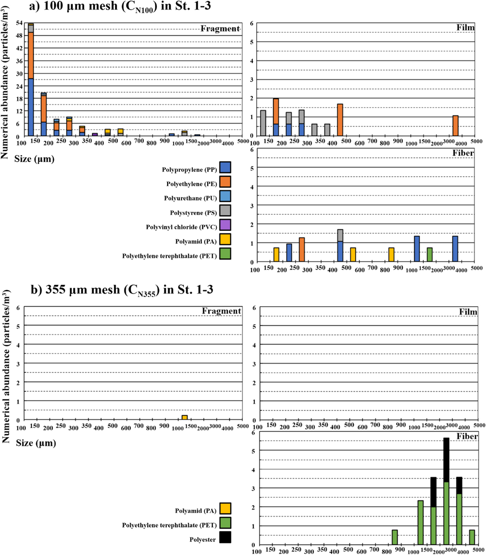
Numerical abundances (CN100, CN355) in St.1–3 (n=9) ranged from 3.2–38.8 (avg. 14.1±10.7, median 13.9) in CN100, and 0.0–12.4 (avg. 1.9±4.0, median 0.4) particles/m3 in CN355. However, mass abundances (CW100, CW355) ranged from 0.2–101.6 (avg. 25.1±41.5, median 6.0) in CW100, and 0.0–26.7 (avg. 3.8±8.7, median 1.0) μg/m3 in CW355 (Table 1). Notably, statistically significant differences were observed with numerical (p=0.001<0.05) and mass (p=0.062<0.1) abundances (Fig. 1). Moreover, the sum of numerical microplastic abundances (n=9), i.e., regardless of the sampling station, was 127.3 particles/m3 and 16.8 particles/m3 in CN100 and CN355, respectively, (Table S1). These abundances are grouped using size, shape, and polymer type in Fig. 2.

Although the size distribution of microfibers was widely dispersive, the film shape showed a relatively smaller size (i.e., below 500 μm) in the 100 μm mesh (Fig. 2a). Contrary to this finding, fragment abundance increased toward the smaller-sized particles, and the 100–150 μm group was the predominant size (Fig. 2a). However, no film shape was observed with the 355 μm mesh, and microfibers were shown with 800–5,000 μm size. Also, while the most frequent size group of the fiber was 2,000–3,000 μm, its specific distribution was not shown (Fig. 2b).
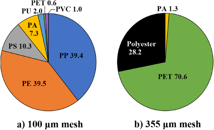
Shape compositions were 84.8% fragment, 7.8% film, 7.4% fiber in the 100 μm mesh, 98.7% fiber, 1.3% fragment in the 355 μm mesh (Fig. 3). Represented microplastics in this study are photographed in Fig. S3. With polymer types (Fig. 4), seven polymers were detected in the 100 μm mesh. Major polymers were 39.5% PE, 39.4% PP, 10.3% PS, followed by 7.3% PA, 2.0% PU, 1.0% PVC, 0.6% PET. However, the 355 μm mesh had fewer polymer types than the 100 μm mesh. These polymers were 70.6% PET, 28.2% polyester, and 1.3% PA. Since some Raman sample spectra in the 355 μm mesh samples were insufficient to identify the obvious PET spectrum due to the fluorescence, they were categorized as polyester.
PERSPECTIVE 1: NUMERICAL AND MASS MICROPLASTIC ABUNDANCES
When median values were compared, CN100 and CW100 were approximately 35 and 6 times higher than CN355 and CW355, respectively (Fig. 1). This tendency reflected a natural increase due to the different mesh sizes, which agreed with previous studies that reported differences between the large and small meshes (Kang et al., 2015; Barrows et al., 2017; Poulain et al., 2019; Lindeque et al., 2020; Tokai et al., 2021).
However, understanding the extent of differences as a macro-perspective compared with other studies on microplastic abundances is needed. Nihei et al. (2020) collected microplastics using a 335 μm mesh from ninety sampling sites on seventy rivers in Japan to compute annual emissions from land to the ocean. Therefore, microplastic numerical (CN100, CN355) and mass (CW100, CW355) abundances in this study were compared with those from the Japanese rivers (Fig. 5).

When microplastic abundance rankings were listed from the lower order, the numerical and mass abundances in this river were ranked 88th (CN100), 10th (CW100), 19th (CN355), and 9th (CW355). Apart from the natural difference observed in numerical abundances, the rankings of mass abundances did not represent a relatively remarkable difference (10th in CW100 and 9th in CW355). Notably, both mass abundances were less than 0.1 mg/m3, which was the median value of the mass abundance in the previous study (Nihei et al. 2020). Additionally, abundances were considerably lower than that from the top 20 sampling points, which had above 1.0 mg/m3 mass abundance (Nihei et al. 2020).
A previous study reported that microplastic numerical and mass abundances correlated with freshwater quality in BOD and DO (Kataoka et al., 2019). In this regard, water quality parameters were evaluated for the past 28 years in the T River to determine the clean river characteristics (Fig. S4). Results showed that the entire parameters reached the AA grade for the three decades, except total coliform. Based on the Environmental Quality Standards for Conservation of the Living Environment (Rivers), the water use of AA grade is a first-class water supply or nature conservation (Kataoka et al., 2019; MOEJ, 2021). Although median mass abundance values differed six times in this study (Fig. 1b), Fig. 5 implied that this difference could be neglected due to the clean river characteristics.
However, neglecting the mass difference between both mesh nets will significantly underestimate microplastic distributions in some freshwaters, which are not pristine, because of numerous mathematical magnifications (Kang et al., 2015; Barrows et al., 2017; Lindeque et al., 2020). Therefore, the 100 μm mesh is recommended from the numerical and mass abundances perspective.
PERSPECTIVE 2: MICROPLASTIC DISTRIBUTIONS ALONG THE FLOW DIRECTION
Median microplastic abundances in each sampling station (n=3) along the river flow are presented in Fig. 6. The CN100 and CW100 increased from the upper (12.5 particles/m3, 6.0 μg/m3) to the lower (14.9 particles/m3, 11.0 μg/m3) area. Previous studies have reported that urban and population ratios significantly affect microplastic abundances (Kataoka et al., 2019). Although the land use at St.2 and St.3 was mainly mountains and forests, St.1 was located close to the urban area (Fig. 6). Furthermore, tributaries between St.3 and St.1 combined with the mainstream and flowed into the estuary through St.1. These land use and tributaries were therefore expected to cause a gradual increase in microplastic abundances in the 100 μm mesh (Yan et al., 2019; Tien et al., 2020; Kameda et al., 2021).
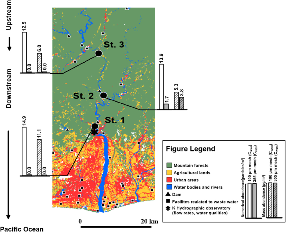
As observed, the CN355 and CW355 showed the highest values in the middle area (1.7 particles/m3, 3.8 μg/m3). A small fiber cluster was identified in one of three replicated samplings in St.2 while picking plastic candidates with a stereomicroscope. The separation into individuals was subsequently conducted, the 16 individual fibers were identified as polyester. This cluster is proposed to be a derivative of ‘fabric pilling’ that commonly occurs in lifestyle textile products (Sillanpaa and Sainio, 2017; Corami et al., 2020). Indeed, a PET cluster morphologically similar to that of this study was discovered in crabs (C. dehaani) from Osaka Bay, Japan (Nakao et al., 2020).
Furthermore, since this study employed two analytical methods (Kudo et al., 2018; Sugiura and Takada, 2019) to optimize microplastic distributions using two different size meshes, accidental irregularities were considered derivatives of the difference between both meshes. These accidentally discovered irregularities in the 355 μm mesh generated uncertain distribution characteristics.
PERSPECTIVE 3: MICROPLASTIC SIZES
Large plastics degrade into smaller particles, and the numbers of small plastic fragments increase as their size decreases (Andrady, 2011; Isobe, 2016; GESAMP, 2019). In this study, the 100 μm mesh revealed the specific size distribution of fragments, thereby reflecting this tendency, unlike the 355 μm mesh (Fig. 2). Though film and fragment plastics >350 μm were collected in the 100 μm mesh, only one fragment was found in the 355 μm mesh.
Several researchers have suggested that particles above the mesh size can pass due to the changed orientation caused by rotation in the water column (Michida et al., 2019; Abeynayaka et al., 2020). With the 355 μm mesh, the maximum length in which particles passed was extended to approximately 502 μm, using the Pythagorean Theorem (Fig. S5). The minimum Feret diameter (FS) was a principal factor in this case (Tokai et al., 2021). Hence, if the FS was shorter than that of the 502 μm, particles were expected to pass the mesh using the cater-corner orientation through rotation (Fig. S5, Case 4). This possibility can also apply to the 100 μm mesh, and the extended mesh was approximately 141 μm (Fig. S5). Thus, considering the underestimated microplastics in mesh sizes, two factors (particles rotation and FS) should be conferred simultaneously (Michida et al., 2019; Abeynayaka et al., 2020; Tokai et al., 2021).
Cumulative probabilities of FL and FS for the fragment and film in the 100 μm mesh were enumerated to presume how many were potentially underestimated in both meshes (Fig. 7). Fibers are not illustrated in Fig. 7 because they were selectively collected in the two meshes (Tokai et al., 2021). When the extended maximum lengths were considered, i.e., the diagonal lengths, probabilities in FS were 67.3% and 96.7% with 141 μm and 502 μm, respectively. These probabilities significantly increased from FL, which showed 8.5% and 86.7% with 100 μm and 355 μm, respectively.

Notably, Fig. 7 was divided into three parts based on the extended length (141 μm and 502 μm) and Fs. Theoretically, parts 1 and 2 indicated collectable fragments and films using 355 μm and 100 μm meshes, respectively. In addition, part 3 implied potential fragments and films that can be overlooked theoretically in the 100 μm mesh. These three parts suggested the following: 1) 96.7% of the fragments and films were underestimated in the 355 μm mesh than the 100 μm mesh and 2) 67.3% of the fragments and films, which were expected to pass the 100 μm mesh, was potentially overlooked.
These arguments reflect the microplastic underestimation in a large mesh (Lindeque et al., 2020; Tokai et al., 2021) and the unavoidable overlooking of microplastics with the volume-reduced sampling method (Hidalgo-Ruz et al., 2012; Song et al., 2014; Kang et al., 2015; Barrows et al., 2017). It implied that the 355 μm mesh is unsuitable for collecting 96.7% of the fragment and film particles based on size perspective.
PERSPECTIVE 4: MICROPLASTIC SHAPES
According to the shape composition (Fig. 3), primary shapes had an 84.8% fragment in the 100 μm mesh and 98.7% fiber in the 355 μm mesh. Although the reason for the absence of fragments and films in the 355 μm mesh was discussed above, microfiber proportions were remarkably different between both meshes.
Apart from the 16 fibers that were captured as one fiber cluster mentioned above using the 355 μm mesh in St.2, the numerical microfiber abundances (Fig. 8a) ranged from 0.0–2.9 (avg. 1.1±1.1, median 0.9) and 0.0–1.7 (avg. 0.5±0.7, median 0.0) particles/m3 in the 100 μm and 355 μm meshes, respectively. As observed, no statistically significant difference existed (p=0.288). This tendency was consistent with mass microfiber abundances (p=0.963), which were 0.0–85.6 (avg. 9.6±28.5, median 0.1) μg/m3 in the 100 μm mesh and 0.0–3.8 (avg. 0.8±1.3, median 0.0) μg/m3 in the 355 μm mesh (Fig. 8b).

Meanwhile, Dris et al. (2018) stated that less filtered water volume (compared with large mesh) and the clogging problem induced fewer numerical microfiber abundances in a small mesh. Filtered water volumes were 3.2±1.2 m3 and 7.7±1.5 m3 in 100 μm and 355 μm meshes, respectively, periods for filtering 1 m3 of water were 120±22 seconds/m3 and 79±19 seconds/m3 in 100 μm and 355 μm meshes, respectively (Table 1). Indeed, numerous particles, which were shorter than the mesh size, were observed in both meshes, indicating that clogging occurred (Treilles et al., 2021). These factors (i.e., less filtered water volumes and the clogging problem) might cause the 100 μm mesh not to capture the relatively long-length microfibers (Fig. 2), but this hypothesis should be determined in the future with strategic sampling plans.
Notably, the string-like fragment has a different mesh selectivity than other-shaped fragments (Tokai et al., 2021), resulting presumably from morphological characteristics that can easily be entangled or bent (Barrows et al., 2017).
Although these fibers were selectively collected in both meshes, the collection of small microplastic particles in the 100 μm mesh implied that the mesh effectively captured tiny microplastics that can bioaccumulate in aquatic organisms (Lindeque et al., 2020).
PERSPECTIVE 5: MICROPLASTIC POLYMER TYPES
The 39.5% PE was the primary polymer in the 100 μm mesh (Fig. 4), followed by 39.4% PP. These two polymers are the most frequently used polymers in everyday life, have light densities (Hidalgo-Ruz et al., 2012; Prata et al., 2019), thereby commonly accounting for the highest percentage of total polymer composition in surface water (Rodrigues et al., 2018; Eo et al., 2019). The subsequent highest composition in the 100 μm mesh was 10.3% PS, which was widely used as food contact materials (Gelbke et al., 2019). The PA is well known for its textile products globally. In Japan, PU is mainly used in constructing, vehicles, and electronics (Furukawa, 2018), PVC is employed in pipes, cable sheaths, and construction (Mitsumata and Hashimoto, 2019).
Globally, PET and polyester fibers, which were primary polymers in the 355 μm mesh, have been frequently used to produce polyester textile products to date (Semba et al., 2020). These products originate from lifestyle microplastics, particularly washing machines (Sillanpaa and Sainio, 2017; Corami et al., 2020).
Meanwhile, PP and PE polymers are susceptible to photo-oxidation, resulting in physical and chemical changes (Rodrigues et al., 2018). Additionally, a viewpoint exists that microplastic polymer degradation correlates with its tensile strengths (Kameda et al., 2021). The photolysis will degrade these polymers to become nanoplastics, which have a high bioaccumulation potential in aquatic organisms via ingestion (GESAMP, 2019).
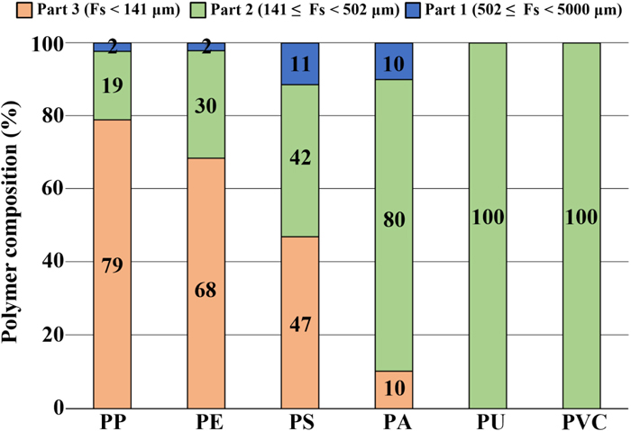
Apart from the fiber, the polymer composition with the fragments and films collected using the 100 μm mesh is illustrated in Fig. 9 based on the three parts in Fig. 7. Parts 2 and 3 accounted for 89%–100% of the total composition in entire polymer types. It implied that 355 μm mesh was insufficient to capture the six polymer types of the fragment and film in the particle size aspect. Therefore, it was also challenging to determine the origins and the bioaccumulation potentials of the polymer type using the 355 μm mesh in this study (Lindeque et al., 2020).
DESIRABLE MESH SELECTION IN THE FRESHWATER
Microplastic numerical and mass abundances in the 100 μm mesh were statistically significantly higher than that of the 355 μm mesh. Recently, an emphasis on Fine Microplastics (FMPs) >20 μm in freshwater has been indicated (Kameda et al., 2021), which shows that previous studies using large meshes to estimate the microplastic emission through freshwater might underestimate the emission (Kataoka et al., 2019; Nihei et al., 2020; Kabir et al., 2021). Moreover, underestimating tiny microplastics was indispensable with the volume-reduced sampling method (Hidalgo-Ruz et al., 2012). Therefore, grabbing water may validly describe microplastic distribution in a situation that the abundances should be carefully illustrated, such as the effect of Wastewater Treatment Plants (WWTPs) (Lahens et al., 2018; Jeong et al., 2021; Kameda et al., 2021).
In addition, microplastic shapes, as well as polymer types, are also primary factors to trace microplastic origins (Isobe, 2016; Conkle et al., 2018; Eo et al., 2018; Katsumi et al., 2021). As observed, 100 μm and 355 μm meshes showed different shape and polymer compositions in this study. Thus, sampling microplastics with the 100 μm mesh were more suitable than using the 355 μm mesh. In contrast, Lindeque et al. (2020) revealed similar fragment and fiber compositions in seawater using 100 μm, 333 μm, and 500 μm meshes. The 335 μm mesh collected PP and PE from 29 Japanese rivers (Kataoka et al., 2019) as major polymer types, consistent with the 100 μm mesh result obtained from this study. It indicated that unsuitable fragment and film distributions using the 355 μm mesh in the shape and polymer type perspectives of this study might be due to specific characteristics of the T river, in which a small number of large fragments and films existed in the pristine water (Fig. 9).
In addition, Michida et al. (2019) recommended a 350 μm mesh for collecting microplastics from the surface seawater because floating fish eggs interrupted the collection using the 100 μm mesh. In this regard, several studies employed a 335 μm mesh on the surface freshwater in Japan (Kudo et al., 2018; Kataoka et al., 2019; Nihei et al., 2020). The interrupting factor of the 100 μm mesh was the suspended matter in those studies. These previous studies indicated that the 355 μm mesh had an advantage on numerous suspended matters, which can clog the small mesh, such as terrestrial plants, mud, sand, and so on.
In conclusion, based on the five perspectives, this study certainly recommended the 100 μm mesh for use in pristine surface freshwater. Though sampling with the 355 μm mesh in the freshwater environment was unsuitable in this study, the mesh was advantageous on specific conditions avoiding clogging of the mesh caused by suspended matter. Therefore, these results indicate that the desirable mesh selection during a research plan establishment step should be considered depending on the research purposes, river characteristics, and weather conditions.
CONCLUSION
This study carefully determined differences in detailed microplastic distributions of surface freshwater collected using the 100 μm and 355 μm meshes using five perspectives: numerical/mass abundances, distributions along the flow direction, and microplastic features (size, shape, polymer type). Apart from the numerical abundance that is naturally increased, mass abundance in the 100 μm mesh was six times higher than that of the 355 μm mesh. Furthermore, although the microplastic numerical abundance in the 100 μm mesh showed a gradually increased distribution toward the estuary where the urban area was located, the 355 μm mesh showed a different distribution due to accidental irregularities in the analytical steps. The cumulative probabilities for the minimum Feret diameter of particles (fragment and film) were divided into three parts, indicating 97% and 67% of the potential underestimation in the 355 μm and 100 μm meshes, respectively. It was therefore challenging to trace microplastic origins and estimate bioaccumulation potentials in the size, shape, and polymer type perspectives using the 355 μm mesh. Nevertheless, in this study, although the 100 μm mesh showed more specific distributions than the 355 μm mesh, a suitable sampling method should be employed to describe microplastic distributions depending on the river characteristics and study purposes.
ACKNOWLEDGMENT
A grant from the Mizuki Biotech. Co., Ltd. (Fukuoka, Japan) and the J-POWER/Electric Power Development Co., Ltd. Chigasaki Research Institute (Kanagawa, Japan) was used to support this study.
SUPPLEMENTARY MATERIAL
Table S1, Total numerical microplastic abundances in 100 and 355 μm meshes by size, shape, and polymer types; Fig. S1, The spectra of seven polymer types found in this study; a) FT-IR and b) Raman spectroscopy. a) The reference spectra in the FT-IR library, b) Commercial product spectra; Fig. S2, Employed a maximum Feret diameter (FL) and a minimum Feret diameter (FS) to measure particle sizes in the present study. (a) was extracted from Yap et al. (2013) Diagn Interv Radiol, 19. 2. 97–105, re-illustrated, (b) is an arbitrary particle in this study, (c) is measured the length (L), diameter (D), thickness (T) in an arbitrary rectangular microfiber using the Stereoscopic Zoom Microscope (3.0–15.0 magnifications, SMZ25, Nikon Corp., Tokyo, Japan) with the NIS-Elements BR version 5.30.00 [Bild1531] software (Nikon Corp., Tokyo, Japan). The microfiber length was measured by a continuous line drawn from end-to-end of the fiber outline using the Stereoscopic Zoom Microscope, the diameter was the shortest line between one end of the fiber, the thickness was the edge line between surface and bottom areas; Fig. S3, The photographed representative microplastics by the Stereoscopic Zoom Microscope (3.0–15.0x) in the 100 (a-o) and 355 μm (p-t) net. The Fig. 4j particle could be considered as a pellet in a 2-dimensional image, but it was shaped like a concave bowl in the Stereoscopic Zoom Microscope observation; Fig. S4, The figure assessed water quality parameters on the K Hydrographic observatory, T River, during the past three decades (1990–2018) by the Environmental Quality Standards for Conservation of the Living Environment (Rivers), Japan (Ministry of Environment Japan, 2021); AA-E grades. The parameters were pH, biological oxygen demand (BOD), suspended solids (SS), dissolved oxygen (DO), and total coliform; Fig. S5, The maximum length on the diagonal that appeared in 100 and 355 μm nets. A virtual oval cylinder particle can be collected on the 355 μm net (Case 1–3) and where it is likely to pass through the 355 μm net (Case 4). The figure was extracted from Abeynayaka et al. (2020) Water, 2020. 12. 1903, supplemented and re-illustrated.
This material is available on the Website at https://doi.org/10.5985/emcr.20210008.
REFERENCES
- Abeynayaka, A., Kojima, F., Miwa, Y., Ito, N., Nihei, Y., Fukunaga, Y., Yashima, Y., Itsubo, N., 2020. Rapid sampling of suspended and floating microplastics in challenging riverine and coastal water environments in Japan. Water 12, 1903. doi: 10.3390/w12071903.
- Andrady, A.L., 2011. Microplastics in the marine environment. Mar. Pollut. Bull. 62, 1596–1605. doi: 10.1016/j.marpolbul.2011.05.030.
- Barboza, L.G.A., Lopes, C., Oliveira, P., Bessa, F., Otero, V., Henriques, B., Raimundo, J., Caetano, M., Vale, C., Guilhermino, L., 2020. Microplastics in wild fish from North East Atlantic Ocean and its potential for causing neurotoxic effects, lipid oxidative damage, and human health risks associated with ingestion exposure. Sci. Total Environ. 717, 134625. doi: 10.1016/j.scitotenv.2019.134625.
- Barrows, A.P.W., Neumann, C.A., Berger, M.L., Shaw, S.D., 2017. Grab vs. neuston tow net: a microplastic sampling performance comparison and possible advances in the field. Anal. Methods 9, 1446–1453. doi: 10.1039/c6ay02387h.
- Bessa, F., Barria, P., Neto, J.M., Frias, J., Otero, V., Sobral, P., Marques, J.C., 2018. Occurrence of microplastics in commercial fish from a natural estuarine environment. Mar. Pollut. Bull. 128, 575–584. doi: 10.1016/j.marpolbul.2018.01.044.
- Cho, L., 2007. Identification of textile fiber by Raman microspectroscopy. Forensic Sci. J. 6, 55–62. http://fsjournal.cpu.edu.tw/content/vol6.no.1/6(1)-4.pdf (accessed 31 August 2021)
- Conkle, J.L., del Valle, C.D.B., Turner, J.W., 2018. Are we underestimating microplastic contamination in aquatic environments? Environ. Manage. 61, 1–8. doi: 10.1007/s00267-017-0947-8.
- Corami, F., Rosso, B., Bravo, B., Gambaro, A., Barbante, C., 2020. A novel method for purification, quantitative analysis and characterization of microplastic fibers using Micro-FTIR. Chemosphere 238, 124564. doi: 10.1016/j.chemosphere.2019.124564.
- Danopoulos, E., Jenner, L.C., Twiddy, M., Rotchell, J.M., 2020. Microplastic contamination of seafood intended for human consumption: a systematic review and meta-analysis. Environ. Health Perspect. 128, 126002. doi: 10.1289/EHP7171.
- Desforges, J.P., Galbraith, M., Ross, P.S., 2015. Ingestion of Microplastics by zooplankton in the Northeast Pacific Ocean. Arch. Environ. Contam. Toxicol. 69, 320–330. doi: 10.1007/s00244-015-0172-5.
- Dris, R., Gasperi, J., Rocher, V., Tassin, B., 2018. Synthetic and non-synthetic anthropogenic fibers in a river under the impact of Paris Megacity: sampling methodological aspects and flux estimations. Sci. Total Environ. 618, 157–164. doi: 10.1016/j.scitotenv.2017.11.009.
- Eo, S., Hong, S.H., Song, Y.K., Han, G.M., Shim, W.J., 2019. Spatiotemporal distribution and annual load of microplastics in the Nakdong River, South Korea. Water Res. 160, 228–237. doi: 10.1016/j.watres.2019.05.053.
- Eo, S., Hong, S.H., Song, Y.K., Lee, J., Lee, J., Shim, W.J., 2018. Abundance, composition, and distribution of microplastics larger than 20 Mm in sand beaches of South Korea. Environ. Pollut. 238, 894–902. doi: 10.1016/j.envpol.2018.03.096.
- Furukawa, M., 2018. The beginning of polyurethanes and recent economic trend in Japan. J. Networkpolymer, Jpn. 39, 3–9. doi: 10.11364/networkedpolymer.39.1_3. (in Japanese)
- Gelbke, H.P., Banton, M., Block, C., Dawkins, G., Eisert, R., Leibold, E., Pemberton, M., Puijk, I.M., Sakoda, A., Yasukawa, A., 2019. Risk assessment for migration of styrene oligomers into food from polystyrene food containers. Food Chem. Toxicol. 124, 151–167. doi: 10.1016/j.fct.2018.11.017.
- GESAMP, 2019. Guidelines for the monitoring and assessment of plastic litter in the ocean. United Nations Environment Programme (UNEP), Nairobi. http://www.gesamp.org/publications/guidelines-for-the-monitoring-and-assessment-of-plastic-litter-in-the-ocean (accessed 1 May 2021)
- Hidalgo-Ruz, V., Gutow, L., Thompson, R.C., Thiel, M., 2012. Microplastics in the marine environment: a review of the methods used for identification and quantification. Environ. Sci. Technol. 46, 3060–3075. doi: 10.1021/es2031505.
- Isobe, A., 2016. Percentage of microbeads in pelagic microplastics within Japanese coastal waters. Mar. Pollut. Bull. 110, 432–437. doi: 10.1016/j.marpolbul.2016.06.030.
- Jeong, H., Novirsa, R., Cahya Nugraha, W., Addai-Arhin, S., Phan Ding, Q., Fukushima, S., Fujita, E., Bambang, W., Kameda, Y., Ishibashi, Y., Arizono, K., 2021. The distributions of microplastics (MPs) in the Citarum River Basin, West Java, Indonesia. J. Environ. Safety 12, 33–43. doi: 10.11162/daikankyo.E21RP0102.
- Kabir, A., Sekine, M., Imai, T., Yamamoto, K., Kanno, A., Higuchi, T., 2021. Assessing small-scale freshwater microplastics pollution, land-use, source-to-sink conduits, and pollution risks: Perspectives from Japanese rivers polluted with microplastics. Sci. Total Environ. 768, 144655. doi: 10.1016/j.scitotenv.2020.144655.
- Kameda, Y., Yamada, N., Fujita, E., 2021. Source- and polymer-specific size distributions of fine microplastics in surface water in an urban river. Environ. Pollut. 284, 117516. doi: 10.1016/j.envpol.2021.117516.
- Kang, J.H., Kwon, O.Y., Lee, K.W., Song, Y.K., Shim, W.J., 2015. Marine neustonic microplastics around the southeastern coast of Korea. Mar. Pollut. Bull. 96, 304–312. doi: 10.1016/j.marpolbul.2015.04.054.
- Kataoka, T., Nihei, Y., Kudou, K., Hinata, H., 2019. Assessment of the sources and inflow processes of microplastics in the river environments of Japan. Environ. Pollut. 244, 958–965. doi: 10.1016/j.envpol.2018.10.111.
- Katsumi, N., Kusube, T., Nagao, S., Okochi, H., 2021. Accumulation of microcapsules derived from coated fertilizer in paddy fields. Chemosphere 267, 129185. doi: 10.1016/j.chemosphere.2020.129185.
- Kudo, K., Takaoka, T., Nihei, Y., Kitaura, F., 2018. Estimation of temporal variations and annual flux of microplastics in rivers under low- and high-flow conditions. J. Jpn. Soc. Civil Eng., Ser. B1 (Hydraulic Eng.) 74, 529–534. doi: 10.2208/jscejhe.74.I_529. (in Japanese)
- Lahens, L., Strady, E., Kieu-Le, T.C., Dris, R., Boukerma, K., Rinnert, E., Gasperi, J., Tassin, B., 2018. Macroplastic and microplastic contamination assessment of a tropical river (Saigon River, Vietnam) transversed by a developing megacity. Environ. Pollut. 236, 661–671. doi: 10.1016/j.envpol.2018.02.005.
- Lee, J., Choi, Y., Jeong, J., Chae, K.J., 2021. Eye-glass polishing wastewater as significant microplastic source: Microplastic identification and quantification. J. Hazard. Mater. 403, 123991. doi: 10.1016/j.jhazmat.2020.123991.
- Lindeque, P.K., Cole, M., Coppock, R.L., Lewis, C.N., Miller, R.Z., Watts, A.J.R., Wilson-McNeal, A., Wright, S.L., Galloway, T.S., 2020. Are we underestimating microplastic abundance in the marine environment? A comparison of microplastic capture with nets of different mesh-size. Environ. Pollu. 265, 114721. doi: 10.1016/j.envpol.2020.114721.
- Michida, Y., Chavanich, S., Chiba, S., Cordova, M.R., Cózar, C.A., Galgani, F., Hagmann, P., Hinata, H., Isobe, A., Kershaw, P., Kozlovskii, N., Li, D., Lusher, A. L., Marti, E., Mason, S.A., Mu, J.L., Saito, H., Shim, W.J., Syakti, A.D., Takada, H., Thompson, R., Tokai, T., Uchida, K., Vasilenko, K., Wang, J., 2019. Guidelines for harmonizing ocean surface microplastic (Version 1.1, June 2020). MOEJ (Ministry of the Environment, Japan), Tokyo. https://www.env.go.jp/en/water/marine_litter/guidelines/guidelines.pdf (accessed 1 May 2021)
- Mitsumata, Y., Hashimoto, S., 2019. Assessment of secondary reserves of polyvinyl chloride in Japan. J. Jpn Soc. Civil Eng., Ser. G (Environ. Res.) 75(6), II_7–II_15. doi: 10.2208/jscejer.75.6_II_7. (in Japanese)
- MOEJ (Ministry of the Environment, Japan), 2021. The environmental quality standards for conservation of the living environment (Rivers). MOEJ (Ministry of the Environment, Japan), Tokyo. https://www.env.go.jp/kijun/wt2-1-1.html (accessed 1 May 2021) (in Japanese)
- Nakao, S., Ozaki, A., Yamazaki, K., Masumoto, K., Nakatani, T., Sakiyama, T., 2020. Microplastics contamination in tidelands of the Osaka Bay area in western Japan. Water Environ. J. 34, 474–488. doi: 10.1111/wej.12541.
- Nihei, Y., Yoshida, T., Kataoka, T., Ogata, R., 2020. High-resolution mapping of Japanese microplastic and macroplastic emissions from the land into the sea. Water 12, 951. doi: 10.3390/w12040951.
- Otsuka, Y., Takada, H., Nihei, Y., Kameda, Y., Nishikawa, K., 2021. Current status and issues of microplastic pollution research. J. Jpn. Soc. Water Environ. 44, 35–42. doi: 10.2965/jswe.44.35. (in Japanese)
- Park, T.J., Lee, S.H., Lee, M.S., Lee, J.K., Lee, S.H., Zoh, K.D., 2020. Occurrence of microplastics in the Han River and riverine fish in South Korea. Sci. Total Environ. 708, 134535. doi: 10.1016/j.scitotenv.2019.134535.
- Poulain, M., Mercier, M.J., Brach, L., Martignac, M., Routaboul, C., Perez, E., Desjean, M.C., Ter Halle, A., 2019. Small microplastics as a main contributor to plastic mass balance in the North Atlantic Subtropical Gyre. Environ. Sci. Technol. 53, 1157–1164. doi: 10.1021/acs.est.8b05458.
- Prata, J.C., da Costa, J.P., Duarte, A.C., Rocha-Santos, T., 2019. Methods for sampling and detection of microplastics in water and sediment: a critical review. TrAC, Trends Anal. Chem. 110, 150–159. doi: 10.1016/j.trac.2018.10.029.
- Rodrigues, M.O., Abrantes, N., Goncalves, F.J.M., Nogueira, H., Marques, J.C., Goncalves, A.M.M., 2018. Spatial and temporal distribution of microplastics in water and sediments of a freshwater system (Antuã River, Portugal). Sci. Total Environ. 633, 1549–1559. doi: 10.1016/j.scitotenv.2018.03.233.
- Scott, N., Porter, A., Santillo, D., Simpson, H., Lloyd-Williams, S., Lewis, C., 2019. Particle characteristics of microplastics contaminating the mussel Mytilus edulis and their surrounding environments. Mar. Pollut. Bull. 146, 125–133. doi: 10.1016/j.marpolbul.2019.05.041.
- Semba, T., Sakai, Y., Ishikawa, M., Inaba, A., 2020. Greenhouse gas emission reductions by reusing and recycling used clothing in Japan. Sustainability 12, 8214. doi: 10.3390/su12198214.
- Sillanpaa, M., Sainio, P., 2017. Release of polyester and cotton fibers from textiles in machine washings. Environ. Sci. Pollut. Res. Int. 24, 19313–19321. doi: 10.1007/s11356-017-9621-1.
- Song, Y.K., Hong, S.H., Jang, M., Kang, J.H., Kwon, O.Y., Han, G.M., Shim, W.J., 2014. Large accumulation of micro-sized synthetic polymer particles in the sea surface microlayer. Environ. Sci. Technol. 48, 9014–9021. doi: 10.1021/es501757s.
- Sugiura, M., Takada, H., 2019. Analysis of um-size microplastics in Tamagawa river, In: Japan Society for Environmental Chemistry (ed.), 28th Symposium on Environmental Chemistry, p. 125, Nakanishi Printing Company, Ltd., Sapporo. (in Japanese)
- Sugiura, M., Takada, H., Takada, N., Mizukawa, K., Tsuyuki, S., 2021. Microplastics in urban wastewater and estuarine water: importance of street runoff. Environ. Monit. Contam. Res. 1, 54–65. doi: 10.5985/emcr.20200006.
- Tien, C.-J., Wang, Z.-X., Chen, C. S., 2020. Microplastics in water, sediment and fish from the Fengshan River system: relationship to aquatic factors and accumulation of polycyclic aromatic hydrocarbons by fish. Environ. Pollut. 265, 114962. doi: 10.1016/j.envpol.2020.114962.
- Tokai, T., Uchida, K., Kuroda, M., Isobe, A., 2021. Mesh selectivity of neuston nets for microplastics. Mar. Pollut. Bull. 165, 112111. doi: 10.1016/j.marpolbul.2021.112111.
- Treilles, R., Gasperi, J., Gallard, A., Saad, M., Dris, R., Partibane, C., Breton, J., Tassin, B., 2021. Microplastics and microfibers in urban runoff from a suburban catchment of Greater Paris. Environ. Pollut. 287, 117352. doi: 10.1016/j.envpol.2021.117352.
- Walton, W. H., 1948. Feret’s statistical diameter as a measure of particle size. Nature 162, 329–330. doi: 10.1038/162329b0.
- Yamashita, R., Tanaka, K., Takada, H., 2016. Marine plastic pollution-dynamics of plastic debris in marine ecosystem and effect on marine organisms. Jpn. J. Ecology 66, 51–68. doi: 10.18960/seitai.66.1_51. (in Japanese)
- Yan, M., Nie, H., Xu, K., He, Y., Hu, Y., Huang, Y., Wang, J., 2019. Microplastic abundance, distribution and composition in the Pearl River along Guangzhou city and Pearl River estuary, China. Chemosphere 217, 879–886. doi: 10.1016/j.chemosphere.2018.11.093.
- Zhang, N., Li, Y.B., He, H.R., Zhang, J.F., Ma, G.S., 2021. You are what you eat: microplastics in the feces of young men living in Beijing. Sci. Total Environ. 767, 144345. doi: 10.1016/j.scitotenv.2020.144345.