Full papers
Linkage disequilibrium in a population undergoing periodic fragmentation and admixture
2012 Volume 87 Issue 2 Pages 125-135
Details
2012 Volume 87 Issue 2 Pages 125-135
Glacial and interglacial cycles are considered to have caused the fragmentation and admixture of populations in many organisms. A simple model incorporating such periodic changes of the population structure is analysed in order to investigate the behaviour of neutral genetic variation at one and two loci. The equilibrium is reached very quickly in terms of cycles if the length of a cycle is long, as would be expected of the glaciation cycles. Heterozygosity and linkage disequilibrium are shown to depend on the length of time of the fragmented and admixed phases, population sizes, and number (n) of subpopulations in the fragmented phase. If the population size is small in the fragmented phase and its duration is long, the squared correlation coefficient of two loci (a measure of linkage disequilibrium) just after the admixture is approximated by 1/(n–1) for n > 1. After admixture, the correlation decays at a rate of approximately twice the recombination rate. Therefore, if post-glaciation admixture created linkage disequilibrium, we expect to observe linkage disequilibrium even between moderately linked loci, and its decay pattern along the chromosome is very different from that in a random mating population at equilibrium. This is especially true in organisms with long generation times such as trees.
From about 0.7 million years ago (MYA), approximate 100-k year cycles of ice sheet expansion and recession have been continuous (Webb and Bartlein, 1992). For many species, these cycles (glacial-interglacial cycles) have caused contractions and expansions of their ranges and have resulted in changes in their population structures. More concretely, in one phase (the fragmented phase), the species might retreat to one or a few isolated refugia and their population sizes might become small. In the other phase (the panmictic phase), the subpopulations expand and admix to form a large panmictic population. As an example of approximate panmixis, currently many wind-pollinated plants show only weak population structure (Hamrick and Godt, 1996). Thus, the populations undergo fragmentation and admixture periodically.
In the fragmented phase, variation within subpopulations decreases and variation between subpopulations increases. Admixture merges the variation between subpopulations into variation in the whole population. In such cases, the equilibrium variation is determined by population sizes in the two phases and the time lengths. Jesus et al. (2006) quantified this situation and have shown that variation can be greater than that expected for a panmictic population of constant size even when the population size is small in the fragmented phase (the structured phase of Jesus et al., 2006). Moreover, because population admixture has been known to create linkage disequilibrium (Nei and Li, 1973), we expect to observe stronger linkage disequilibrium compared to that in a panmictic population, especially during the early portion of the panmictic phase.
In the present paper, an analysis of a simple model of genetic variation at one and two neutral loci under periodic admixture-fragmentation is presented. Specific questions asked are; 1. What would be the equilibrium diversity and linkage disequilibrium just after admixture? 2. How quickly is this equilibrium reached? 3. How does the dependency of linkage disequilibrium on the recombination rate under this model differ from that in a panmictic population?
We consider a monoecious diploid population with discrete non-overlapping generations and assume that the population’s structure changes periodically. Each cycle consists of two phases in the following order: the panmictic and the fragmented phases (Fig. 1). At the beginning of the panmictic phase, existing subpopulations in the fragmented phase are merged in equal proportions to form a panmictic population with size N1 and this state continues for t1 generations. At the beginning of the fragmented phase, the population is subdivided into n subpopulations each of which has size N2 and this state continues for t2 generations. In this phase, there is no migration between subpopulations and mating is random in each subpopulation. This cycle is repeated with the same parameters. This model is the same as the one studied by Jesus et al. (2006). We would like to know the diversity measurements of the population at one and two loci (defined below) after k cycles of the fragmentation admixture.
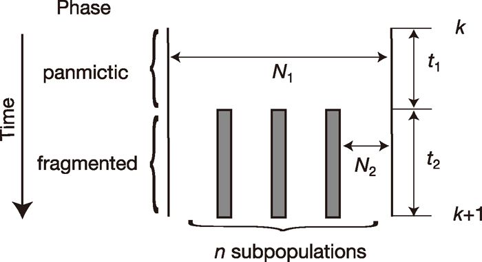
One cycle of fragmentation admixture. A cycle consists of the panmictic and fragmented phases with lengths of t1 and t2 generations, respectively. In the panmictic phase, there is one large panmictic population with size N1, and in the fragmented phase there are n subpopulations each with size N2.
Consider two neutral loci A and B and the recombination rate between them is r. For mutations, the infinite allele model (Kimura and Crow, 1964) is assumed, and u (> 0) is the mutation rate per generation at each locus.
We compute the average heterozygosity at one locus (one-locus diversity measure) and joint heterozygosity (two-locus diversity measure) at two loci under the model by deriving their transition equations. Equivalent results can also be obtained by a genealogical approach as in Jesus et al. (2006) and McVean (2002) or using the diffusion approximation of the Wright-Fisher model as in Ohta and Kimura (1969) and Mano (2007).
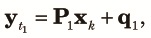
In the following, one- and two-locus diversity measures at the beginning of the kth cycle are calculated. Once they are obtained, it is easy to compute those measures at any time in the cycle using the measures at the beginning of the kth cycle as initial values.
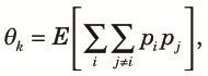
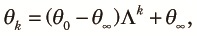
One-locus diversity measuresHere, we consider one of the two loci. Let θk be the probability that two alleles randomly taken from the population at the beginning of the kth cycle are different. At this time point, the panmictic phase has just started. Let pi be the frequency of the ith allele Ai. Then, θk is expressed as:
 |
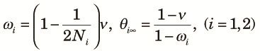 |
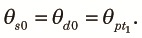
First, we consider the panmictic phase and let θpt be the probability of sampling two different alleles from the population at the tth generation from the start of the panmictic phase. Then,
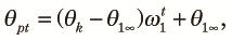 | (1) |
Next, we consider the fragmented phase and let θst and θdt be the probabilities of sampling two different alleles from the same subpopulation and different subpopulations, respectively, at the tth generation from the start of the fragmented phase of the kth cycle. Because two alleles taken at the beginning of the fragmented phase are samples from the panmictic population at the end of the panmictic phase irrespective of whether they are taken from the same or different subpopulations, we obtain:
 | (2) |
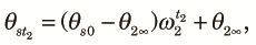 | (3) |
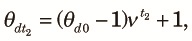 | (4) |
Combining (2)–(4) and noting that the subpopulations contribute equally to the panmictic population at the beginning of the k+1th cycle, we obtain a transition equation:
 | (5) |
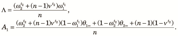 | (6) |
 | (7) |
Note that Λ is less than or equal to the larger of ω1t1ω2t2 and ω1t1νt2 and appreciably smaller than one unless t1 + t2 is small. Therefore, the approach to the equilibrium is fast and the equilibrium value is of practical interest. Numerical examples of the equilibrium value, θ∞, as a function of t2 /t1 for various values of n when t1 /(2N1) = 0.1, N2 /N1 = 0.01 and 4N1u = 0.04 are shown in Fig. 2. Here, we assumed N1, N2 >> 1 and u << 1, so that θ∞ can be approximately expressed as a function of scaled times, t1/(2N1) and t2/(2N2), and the scaled mutation rate 4N1u. The case with n = 1 is just the periodic size change circumstance, and thus θ∞ decreases as t2 increases. If n > 1, θ∞ first decreases as t2 increases, but then it increases and becomes larger than that expected in a randomly mating population with a larger size N1. This is because variation within subpopulations is lost but variation between subpopulations accumulates as time passes in the fragmented phase. The accumulation of variation between subpopulations is faster when n is larger. When n = ∞, the initial decrease does not occur because two alleles taken at the beginning of the cycle never come from the same subpopulation in the fragmented phase. Jesus et al. (2006) have also shown these using a genealogical approach.
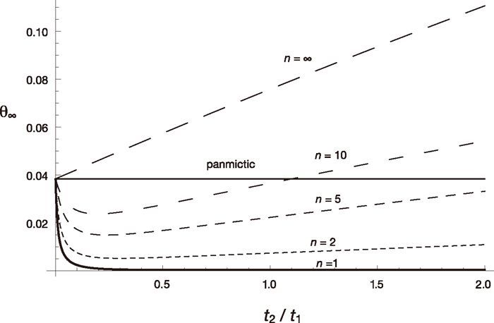
One-locus equilibrium diversity measure, θ∞, as a function of t2 /t1 for various values of n are shown. Other parameters are u = 10–7, N1 = 105, t1 = 2 × 10⁴, N2 = 103.
Next we consider two loci A and B. Let the alleles of the two loci be designated by Ai and Bj, respectively. Define gij, pi, and qj as frequencies of a gamete AiBj, allele Ai, and allele Bj, respectively.
In order to define the diversity measures for two loci, we introduce additional information. Assume that we sample two alleles a, a′ at the A locus and b, b′ at the B locus from the population. There are several ways in which sampled alleles are located on the chromosomes in the population (Weir and Cockerham, 1969). If alleles are on the same chromosome, we concatenate the two alleles. For example, if a and b are on the same chromosome, we write them as ab. If they are on different chromosomes from the same (sub)population, we separate the two alleles by a comma, such as a,b. Finally, alleles in the same (sub)population are put within parentheses. Thus, two alleles (a,b) are from the same (sub)population and (a)(b) are from two different (sub)populations. We indicate that two alleles x, y are different by x ≠ y.
With these notations, we define three two-loci diversity measures at the beginning of the kth cycle as (see Weir and Cockerham, 1969):
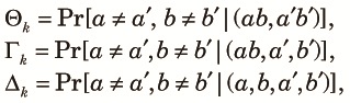 |
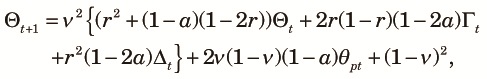
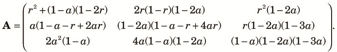
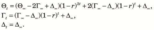
In order to compute the transition from xk to xk+1, we first consider the panmictic phase. Let Θt, Γt, and Δt be the diversity measures at the tth generation from the start of the kth cycle. Here, we derive the transition equation for the digametic measure, which relates Θt+1 to Θt. Those for Γt, and Δt can be derived similarly. We consider three cases, (a) no mutation occurs at either locus (with a probability ν2), (b) mutation occurs at one of the loci and it does not occurs at the other loci (with a probability 2ν (1–ν)) and (c) mutation occurs at both loci (with a probability (1–ν)2).
In case (a), if neither of the two gametes is a recombinant (with a probability (1–r)2), both two allele pairs, (a, a′) and (b, b′), are different when the two gametes come from different chromosomes (with a probability 1–1/(2N1)) and the digametic two allele pairs in the previous generation are different (with a probability Θt). If one of the two gametes is a recombinant but the other is not (with a probability 2r(1–r)), the two allele pairs are different when they come from different individuals (with a probability 1–1/N) and the trigametic two allele pairs in the previous generation are different (with a probability Γt). Note that if both gametes come from the same individual in the previous generation, either of the two allele pairs comes from the same allele in the previous generation. If both gametes are recombinants (with a probability r2), the two allele pairs are different either if they come from different individuals (with a probability 1–1/N) and the quadrigametic two allele pairs in the previous generation are different (with a probability Δt), or if both gametes come from the same individual (with a probability 1/N) but the alleles come from different alleles in this individual (with a probability 1/2) and the digametic two allele pairs in the previous generation are different (with a probability Θt).
In case (b), because one of the two allele pairs are different, only the other allele pair need to be different for the two allele pairs to be different. The other allele pair are different if they come from different alleles in the previous generation (with a probability 1–1/(2N)) and they are different (with a probability θpt). Note that recombination does not affect this case because whether the allele pair at the mutated locus come from the same allele in the previous generation or not does not affect the non-identity of the allele pair. Finally, in case (c), both allele pairs are different independent of how they come from the previous generations. Combining all those with some rearrangements, we obtain the transition equation for Θt as,
 |
 | (8) |
 |
 | (9) |
 |
 | (10) |
In order to calculate the transition equation in the fragmented phase, we need to introduce more two-locus diversity measures because there are several ways in which sampled alleles are located on chromosomes (Tachida and Cockerham, 1986). For simplicity, we assume that the initial condition is symmetric with regard to the two loci. Even with this assumption, we need 13 measures, two digametic, three trigametic and seven quadrigametic measures that are listed in Table 1 along with their allele arrangements.
| subpopulation | digametic | trigametic | quadrigametic |
|---|---|---|---|
| One | Θ1t: (ab,a′b′) | Γ1t: (ab,a′,b′) | Δ1t: (a,b,a′,b′) |
| Two | Θ2t: (ab)(a′b′) | Γ2t: (ab)(a′,b′) | Δ2t: (a,b)(a′,b′) |
| Γ3t: (ab,a′)(b′) | Δ3t: (a,b,a′)(b′) | ||
| Δ4t: (a,a′)(b,b′) | |||
| Three | Γ4t: (ab)(a′)(b′) | Δ5t: (a,b)(a′)(b′) | |
| Δ6t: (a,a′)(b)(b′) | |||
| Four | Δ7t: (a)(a′)(b)(b′) |
Only one representative arrangement is shown for each measure. For example, Γ3t represents a measure for both (ab,a′)(b′) and (ab,b′)(a′).
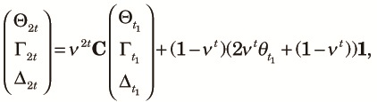
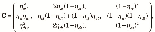
Let t be the time from the beginning of this phase measured in generations. The initial condition for the measures are Θt1, Γt1, and Δt1 for digametic, trigametic and quadrigametic measures, respectively. We want to compute values of those measures zt = (Θ1t, Θ2t, Γ1t, ..., Δ7t, θst, θdt)T at the end of the fragmented phase (t = t2). Although the computation is straightforward, the expressions become complex. Therefore, the derivations are explained in Appendix A. As in the panmictic phase, zt is expressed as a linear function of the initial value
 | (11) |
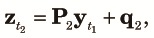
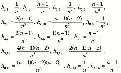
Because n subpopulations contribute equally to the panmictic populations of the next cycle, we obtain the three two-locus diversity measures at the beginning of the k+1th cycle using elements of zt2 as,
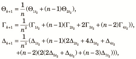 |
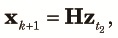 | (12) |
 |
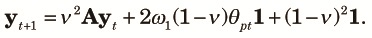
Finally, we combine (10), (11) and (12) to obtain the transition equation from k to k+1 as:
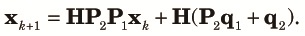 | (13) |
 | (14) |
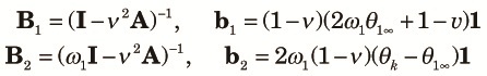
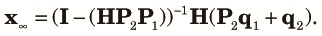
Here, we choose ρ2 (r2 of Hill and Robertson, 1968) as a measure of linkage disequilibrium and compute its approximate expectation using the diversity measures obtained in the preceding sections. The expectation of ρ2 is expressed approximately as (Hill, 1975):
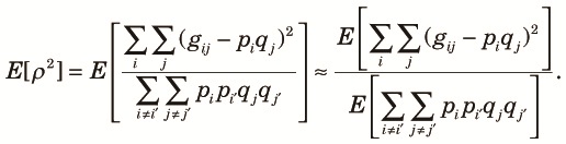 | (15) |
 |
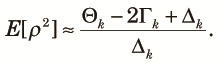 | (16) |
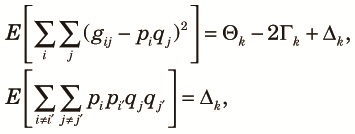
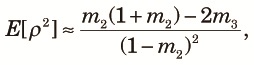
Before showing numerical examples using (16), we consider an extreme case where the recombination rate is large and the subpopulations in the fragmented phase are very small. More formally stated, we assume Nr >> 1 and t2/(2N2) >> 1. Then, at the end of the fragmented phase, each subpopulation becomes monomorphic. Therefore, all diversity measures involving two alleles at the same locus in the same subpopulation become zero. That is:
 | (17) |
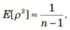 | (18) |
Now let us examine linkage disequilibrium numerically using (13), (14) and (16). First, we ask how quickly the equilibrium state is reached. This can be answered by computing the eigenvalues of the matrix, HP2P1. Let λi (i = 1, ..., 4) be the eigenvalues of the matrix defined in decreasing order. Numerical values of λ1 (the largest) and λ2 (the second largest) are shown in Table 2. Numerical computations show that λ1 is the eigenvalue of θk,
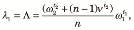 | (19) |
| n = 2 | n = 5 | n = 10 | ||||||
|---|---|---|---|---|---|---|---|---|
| N2 | t2 | r | λ1 | λ2 | λ1 | λ2 | λ1 | λ2 |
| 103 | 8 × 10⁴ | 10–3 | 0.3704 | 0.1372 | 0.5927 | 0.3513 | 0.6667 | 0.4445 |
| 10–5 | 0.2488 | 0.4122 | 0.4772 | |||||
| 10–6 | 0.2967 | 0.4749 | 0.5345 | |||||
| 5 × 10⁴ | 10–3 | 0.3194 | 0.1017 | 0.5101 | 0.2602 | 0.5739 | 0.3293 | |
| 10–5 | 0.1723 | 0.3048 | 0.3601 | |||||
| 10–6 | 0.2481 | 0.3973 | 0.4474 | |||||
| 2 × 10⁴ | 10–3 | 0.2744 | 0.0753 | 0.4391 | 0.1928 | 0.4939 | 0.2440 | |
| 10–5 | 0.1241 | 0.2295 | 0.2733 | |||||
| 10–6 | 0.2075 | 0.3326 | 0.3746 | |||||
| 104 | 8 × 10⁴ | 10–3 | 0.3772 | 0.1423 | 0.5954 | 0.3545 | 0.6681 | 0.4464 |
| 10–5 | 0.2242 | 0.3899 | 0.4633 | |||||
| 10–6 | 0.2968 | 0.4694 | 0.5274 | |||||
| 5 × 10⁴ | 10–3 | 0.3450 | 0.1190 | 0.5206 | 0.2710 | 0.5791 | 0.3354 | |
| 10–5 | 0.1724 | 0.3020 | 0.3567 | |||||
| 10–6 | 0.2638 | 0.3995 | 0.4452 | |||||
Other parameters are N1 = 105, t1 = 105-t2, u = 10–6. λ1 does not depend on r.
To see more directly how quickly E[ρ2] approaches equilibrium at the beginning of the panmictic phase, its change was computed along with the one-locus diversity measure θk. A typical example is shown in Fig. 3. We assumed that the population has been panmictic with size N1 and in the equilibrium state before the start of the first cycle. In this example, λ1 = 0.5927 and λ2 = 0.4122. It takes several cycles to achieve the equilibrium state and E[ρ2] approaches the equilibrium more quickly than θk.

Changes of θk and E[ρ2] at the beginning of the panmictic phase. Parameters are u = 10–6, r = 10–5, N1 = 105, N2 = 103, t1 = 2 × 10⁴, t2 = 8 × 10⁴. Until the beginning of cycle 1, the population has been panmictic with size N1 and in the equilibrium state.
Next we examine the equilibrium state. Figure 4 shows E[ρ2] at the beginning of the panmictic phase as a function of the recombination rate for various values of n. As shown in the figure, E[ρ2] decreases as r increases and approaches 1/(n–1) (see (18)) except in the case of n = 2, because t2/(2N2) = 8 used in the figure is very large. Therefore, strong linkage disequilibria are expected at the beginning of the panmictic phase when t2/(2N2) is large. As n increases, E[ρ2] decreases. When the length, t2, of the fragmented phase becomes shorter, the level of linkage disequilibrium decreases as shown in Fig. 5. Note that admixture results in linkage disequilibrium even without fixation within subpopulations, although its absolute value is not large (see the case of t2 = 2N2).
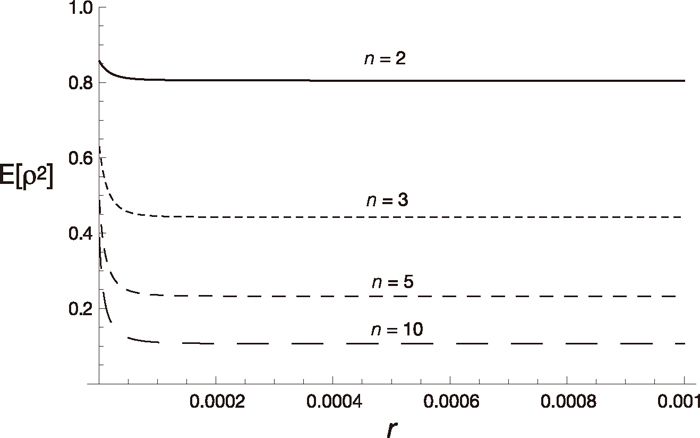
Equilibrium values of linkage disequilibrium, E[ρ2], and the number of subpopulations. E[ρ2] is shown as a function of the recombination rate r. Four cases (n = 2, 3, 5, 10) are shown. Other parameters are u = 10–7, N1 = 105, N2 = 5 × 10³, t1 = 2 × 10⁴, t2 = 8 × 10⁴.
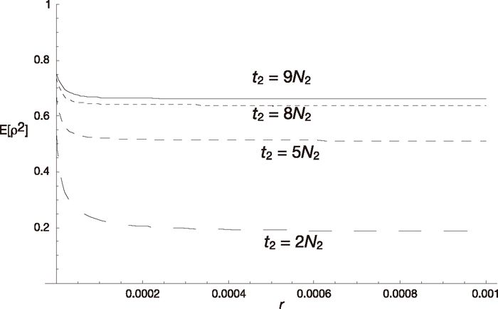
Equilibrium values of linkage disequilibrium, E[ρ2], and the length of the fragmented phase. E[ρ2] is shown as a function of the recombination rate r. Four cases (t2 = 9N2, 8N2, 5N2, 2N2) keeping the total length of one cycle constant are shown. Other parameters are u = 10–7, n = 2, N1 = 105, N2 = 104, t1 = 105-t2.
Finally, we consider E[ρ2] at the tth generation since the start of the panmictic phase. Because the approach to equilibrium in terms of cycles of the fragmentation-admixture is rapid, only the equilibrium state will be considered. We can compute E[ρ2] using the equilibrium value, x∞, as its initial condition and putting it into (9). When 2Nr >> 1, the time course of E[ρ2] can be approximately computed by ignoring the terms containing 1/(2N1) in (9). In this case, the two-locus diversity measures are approximately expressed as:
 |
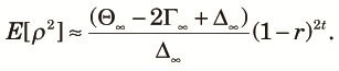 | (20) |
 | (21) |

The decay of linkage disequilibrium, E[ρ2], in the panmictic phase. Values of E[ρ2] at 0, 1000, 2000, 10000th generations since the beginning of the panmictic phase are shown as functions of the recombination rate, r. Straight and broken lines represent values of E[ρ2] computed from (9) along with (16), and (20), respectively. Approximate equilibrium values (Eq.) for N1 = 105 calculated from (21) are also shown. Parameters are u = 10–7, N1 = 105, N2 = 5 × 10⁴, t1 = 2 × 10⁴, t2 = 8 × 10⁴.
In this paper, the diversity measures at one and two loci, and a measure of linkage disequilibrium were investigated in a population undergoing periodic fragmentation and admixture. The study was motivated by the periodic nature of glaciation-interglaciation geological conditions. Under these circumstances, equilibrium is quickly approached and the size, N2, of subpopulations and time length, t2, of the fragmented phase, along with the number of subpopulations, strongly influence the levels of diversity measures and linkage disequilibrium. The parameters, N2, n, and t2, together determine the reduction of variation within subpopulations during the fragmented phase. After only one cycle of fragmentation and admixture, patterns of variation very different from those expected in panmictic populations are observed.
Such large linkage disequilibrium is also expected under models with geographically structured populations (Ohta, 1982; Tachida and Cockerham, 1986; De and Durrett, 2007). However, large estimates of FST (if subpopulations are recognized) or FIS (if subpopulations are not recognized) are expected in geographically structured populations. On the other hand, estimates of those F-statistics are very small under the present model after admixture. Therefore, it is not difficult to discriminate the two types of models from the data. Incidentally, large estimates of linkage disequilibrium may lead to spurious detection of positive selection using the decay of the extended haplotype homozygosity as pointed out by De and Durrett (2007). Therefore, it is important to obtain information of the past population structure to infer actions of selection.
Because we made some simplifying assumptions in drawing those conclusions, we will briefly consider some of their effects here. First, we assumed that transitions between the phases are instantaneous in the model. In reality, the expansion after glaciation is not instantaneous, although it is not slow (Hewitt, 2000). For example, in the case of the Japanese cedar, Cryptomeria japonica, its expansion started from a few refugia about 15000 years ago and its maximum abundance and range was reached around 7000 years ago (Tsukada, 1982). Therefore, N2 is not constant through time. To address this violation, we might use effective size such as the harmonic mean for N2 because an important factor is the extent to which variation is reduced within subpopulations in the fragmented phase. For the change of linkage disequilibrium, formulas in Mano (2007) may be useful.
Second, although all parameters were assumed to be constant throughout the cycles in our model, some parameters might change between cycles. Indeed, glacial-interglacial cycles have been only quasi-periodic and some long-term trends might be imposed on them (see Webb and Bartlein, 1992). In addition, effective population sizes and number of subpopulations in the fragmented phase could fluctuate. Among those parameters, the time lengths are determined mainly by orbital-forcing of climatic oscillations and thus an approximate periodicity seems to be the case. Random factors, however, are likely to contribute to the resulting population sizes and the number of subpopulations as they are biological attributes. Therefore, their values might change randomly among the cycles of fragmentation and admixture. Especially important in determining the magnitude of linkage disequilibrium is the number, n, of subpopulations. Palynological studies (studies based on pollen and spores) have shown that some species were missing in some refugia in certain glacial periods (Bennett, 1997). Although a consideration of parameter fluctuation is important to understand the genetic diversity of organisms affected by repeated fragmentation-admixture, our results suggest that the most recent cycle is of primary importance because equilibrium is reached fairly quickly. Hence, the prediction of strong linkage disequilibrium from our model does not change qualitatively unless n in the most recent fragmentation phase is one.
Finally, although we assumed that n subpopulations in the fragmented phase equally contribute to the panmictic populations when admixture occurs, this is unlikely to be true in nature. Here, we consider the effects of an unequal contribution in the extreme case of Nr >> 1, and t2/(2N2) >> 1. For n = 2, E[ρ2] is still close to one because it is a correlation coefficient. To consider the case with n > 2, let xi be the contribution from the ith subpopulation to the panmictic population. Then, instead of (18), we obtain:
 |
 |
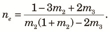 |
Because E[ρ2] is a decreasing function of ne, any unequal contribution that reduces ne will increase E[ρ2].
Many of the extant abundant taxa are considered to have experienced fragmentation during the glaciation period (Webb and Bartlein, 1992). Therefore, admixture of their fragmented subpopulations is considered to have occurred between approximately 5000 and 15000 years ago. Because the half-life of the linkage disequilibrium created by admixture is approximately 0.347/r generations, we expect to observe more than half the level of linkage disequilibrium at the beginning of the interglaciation between two markers less than 34.7/t cM apart, where t is the number of generations since the admixture. Therefore, extended linkage disequilibrium will be found in organisms having longer generation times. Recently, fine linkage maps have been developed in many organisms and total genome sequences are available in some model organisms. Thus, we can choose markers suitable for observing linkage disequilibrium as traces of past fragmentation. For example, if we assume that the generation time of a tree is 50 years, only one to three hundred generations have passed since the admixture after glaciation occurred. Then, we should be able to find linkage disequilibria between markers 0.35-0.11 cM or less apart if it existed when the admixture occurred. Because such markers are now available for trees (e.g. Brown et al., 2001; Tani et al., 2003; Tuskan et al., 2006), it would be interesting to survey those markers in natural populations to investigate their past population structure (see also Lascoux et al., 2008).
Let t be the number of generations since the beginning of the fragmented phase. The initial conditions for the measures are Θt1, Γt1 and Δt1, for digametic, trigametic and quadrigametic measures, respectively. We want to compute values of those measures at the end of the fragmented phase.
The single population measures (Θ1t, Γ1t and Δ1t) are computed using equation (9) but setting a = a2 = 1/(2N2).
Next we compute the two population measures. First, we consider Θ2t, Γ2t and Δ2t. Note that no allele pair at the same locus is in the same subpopulation in these allele arrangements. Thus, no coalescence occurs between a pair of alleles at the same locus and we can obtain the explicit expressions for Θ2t, Γ2t and Δ2t:
 | (A1) |
 |
 |
 |
 | (A2) |
 |
 |
 | (A3) |
 | (A4) |
 |
For the three-population allele arrangements (ab)(a′)(b′) and (a,b)(a′)(b′), again coalescence does not occur. Therefore, Γ5t and Δ5t are obtained using ηst and ηdt as:
 | (A5) |
 | (A6) |
 |
 | (A7) |
 | (A8) |
I thank two anonymous referees for their helpful comments on earlier drafts of the manuscript. This work was partially supported by the Program for Promotion of Basic and Applied Researches for Innovations in Bio-oriented Industry (BRAIN) and by the Environment Research and Technology Development Fund (S-9-2) of the Ministry of the Environment, Japan.